Suitability Evaluation of Multipoint Simultaneous CO2 Sampling Wireless Sensors for Livestock Buildings

 , ,
, ,
Abstract
: The environment in livestock buildings must be controlled to ensure the health and welfare of both workers and animals, as well as to restrict the emission of pollutants to the atmosphere. Among the pollutants generated inside these premises, carbon dioxide (CO2) is of great interest in terms of animal welfare and ventilation control. The use of inexpensive sensors means that complete systems can be designed with a number of sensors located around the building. This paper describes a study of the suitability of multipoint simultaneous CO2 sensors operating in a wireless sensor network, which was found to operate satisfactorily under laboratory conditions and was found to be the best alternative for these applications. The sensors showed a highly linear response to CO2 concentrations, ranging from 500 to 5000 ppm. However, individual sensor response was found to differ, which made it necessary to calibrate each one separately. Sensor precision ranged between 80 and 110 ppm CO2, and sensor response to register a 95% change in concentration was estimated at around 5 min. These features mean this type of sensor network can be used to monitor animal welfare and also for environmental control in poorly ventilated livestock premises. According to the tests conducted in this study, a temporal drift may occur and therefore a regular calibration of sensors would be needed.
1. Introduction
Intensive livestock rearing is associated with the emission of large amounts of atmospheric pollutants, which impair animal health and welfare inside the buildings and have a serious environmental impact. The accumulation of ammonia (NH3) inside livestock houses affects animal health and welfare [1,2], and the emission of this gas is associated with the acidification of soils and the eutrophication of ecosystems [3]. Greenhouse gases such as methane (CH4) and nitrous oxide (N2O), which are generated both by the animals themselves and their manure, contribute to climate change [4]. Due to the accumulation of these effects, many regulations have been issued in recent years (e.g., the Kyoto Protocol, European Ceilings Directive), which directly or indirectly affect the design and operation of livestock buildings.
Carbon dioxide (CO2) is produced in livestock farms mainly as a result of animal respiration and the aerobic decomposition of their manure. Although CO2 is a greenhouse gas, animal-related CO2 emissions are not considered a net addition to the atmosphere, since this gas participates in a short-term closed cycle [5]. However, CO2 has been widely used as a tracer gas to quantify ventilation in livestock buildings [6] and exposure to high concentrations of this gas has also been associated with impaired health of both humans and animals [7].
Ventilation of livestock housing provides fresh air to the animals and removes any potential airborne pollutants released inside the building. Measuring ventilation rates in livestock buildings is therefore essential for proper building design and operational control. Furthermore, ventilation should be quantified and the air should be monitored with a view to determining gas concentrations in order to estimate the emission of other atmospheric pollutants by means of mass balances. Currently, most pollutants can be measured with acceptable precision using a wide variety of measurement techniques [8], but quantifying airflow rates may be more complicated [9].
Measuring ventilation rates in commercial livestock buildings is complex and time-consuming, and is particularly challenging in naturally ventilated livestock buildings, where changing outdoor conditions determine irregular and continuously varying ventilation patterns. Naturally ventilated buildings are commonly used to house certain animal species such as dairy cattle and are widely used for other species under mild or warm conditions. They are also seen as a good solution in developing countries and areas with restricted access to electricity. However, the measurement and control of a ventilation system remains an elusive target for farmers and researchers [10]. As discussed by [9], CO2 can be used as a tracer to determine farm ventilation and pollutant emissions, but more development is needed regarding CO2 production inside the farm and also in terms of CO2 measurement technology.
Farmers are increasingly required to improve the control of ventilation in their buildings. Welfare regulations also include a ventilation system which is able to maintain indoor gas concentrations below certain thresholds (e.g., 20 ppm NH3 and 3000 ppm CO2 for broilers, according to European Council Directive 2007/43/EC [11]. It is also now widely accepted that maintaining appropriate air quality in animal housing is effective, not only to ensure acceptable welfare status, but it also has a positive influence on animal performance.
Measuring CO2 concentrations in livestock buildings is therefore of great interest to farmers. Firstly, this information could be included in the farm climate control system to control ventilation as required. Sly, the accurate determination of ventilation rates by means of CO2 balances would allow alternative housing systems to be characterized in terms of pollutant emissions. In addition, such a system would provide information on animal welfare related to exposure to gaseous pollutants.
CO2 balance has been proposed as alternative method of estimating ventilation rates. The CO2 naturally emitted in livestock houses fulfills the properties of a tracer gas established by [12]: low and stable background concentrations, low risk in case of exposure, easy to handle and measure. The CO2 balance methodology has been widely described [6,13] and applied to a number of mechanically ventilated livestock houses. To apply this method two inputs must be characterized accurately. The first requires that the CO2 produced by the animals and their manure be well characterized; this production can be estimated according to [6] and is proportional to the metabolic activity of the animals, which depends on the type of animal, its weight and its productivity. The s input is an accurate measure of the difference in CO2 concentration between the exhaust and incoming air. This requires a high time and space resolution in concentration measurements.
The air inside livestock houses is characterized by relatively low CO2 concentrations, which are mostly under 5000 ppm [14–17]. In some cases (naturally ventilated, open buildings) indoor CO2 concentrations are lower than 500 ppm, which involves a difference of less than 200 ppm with outdoor air. In most mechanically ventilated buildings the incoming air mixes perfectly with the air already present and CO2 concentration gradients are stable and well characterized. However, in naturally ventilated buildings (particularly those of open structure), indoor and outdoor concentrations are similar, perfect mixing is not achieved and permanent changes in CO2 gradients are common as a consequence of changes in airflow patterns. CO2 concentration measurements in livestock buildings must meet the following requirements:
They should be sufficiently precise for the purpose of the study. For assessing animal welfare, a precision of 100 ppm may be enough, considering that a threshold of 3000 to 5000 ppm is normally established. For ventilation, the precision should be enough to properly characterize the difference between the indoor and outdoor environments. In closed, naturally ventilated buildings, a difference of 150 ppm should be detected [13], but more open structures will require much more precise measurement [9].
Simultaneous multi-point measurements to provide reliable information on the spatial distribution of gas concentrations.
Adequate time resolution to detect changes determined by varying outdoor conditions.
From the livestock producer's point of view, it would be advisable to install a set of CO2 sensors at different points in a building. This would allow an in-depth study of CO2 concentration at these points and would monitor the airflow effect. Of course, to make this a viable approach, the measurement system must have a competitive price. Our proposal includes a wireless sensor network consisting of a set of CO2 sensors placed throughout the building. In order to select the most appropriate CO2 sensor for this work, an in-depth analysis of commercial sensors must be carried out. The sensor will then be connected to the best current technology to store and communicate the results: a wireless sensor network (WSN) architecture.
The huge advances in technologies such as very large scale integrated microelectromechanical systems and wireless communications have contributed to the widespread use of distributed sensor systems [18]. The miniaturization of computing and sensing technologies has enabled the development of tiny, low-powered, inexpensive sensors, actuators, and controllers. Embedded computing systems (i.e., systems that typically interact closely with the physical world and are designed to perform only a limited number of dedicated functions) continue to find applications in an increasing number of areas. While defense and aerospace systems still dominate the market, there is an increasing focus on systems that monitor and protect civil infrastructures such as bridges and tunnels, the national power grid and pipelines. Networks of hundreds of sensor nodes are already being used to monitor large geographic areas for modeling and forecasting environmental pollution and flooding, using vibration sensors to collect structural health information on bridges, and controlling usage of water, fertilizers, and pesticides to improve crop health and quantity.
In this paper, we deal with two particular objectives. First, the selection of an appropriate CO2 sensor to be used in wireless sensor networks, and sly, to evaluate this sensor under laboratory conditions in order to assess its potential application to practical aspects of livestock farming, such as ventilation control, welfare assessment or environmental applications. The paper is structured as follows: Section 2 describes the selection process of the CO2 sensor and the wireless CO2 sensor network is presented in Section 3, including the experimental set-up for evaluating the sensor performance. Section 4 includes the results and discussion and, finally, our conclusions are presented in Section 5.
2. Choice of CO2 Sensor
The type of installation in which the sensors will be deployed requires the measurement of concentrations of CO2 in air for a range between 0 and 5000 ppm with an accuracy of ±100 ppm. The choice of sensor is critical, since our experimental set-up requires a wireless network of CO2 sensors. This imposes the following restrictions:
Energy-constrained wireless sensor nodes. Both the CO2 sensors and wireless nodes must have low energy requirements. The set-up can vary from one recording per min every week to one every 10 min for five months, so that the battery system must be sized to last for a whole campaign.
Small sensor size for embedding in the physical node.
No recalibration while the experiment is running. Error specifications must be limited and known for the full experiment, which can mean as long as five months of known measurement behavior. Measurement accuracy must be as high as possible without the need for recalibration during the entire experiment [19].
Long sensor life. Some CO2 sensors have a limited life due to chemical contamination. This degradation influences measurement, implying extra maintenance.
Low-cost. To obtain simultaneous multi-point measurements a considerable number of nodes are needed, so sensor price is important.
Accurate sensors. Known accuracy is necessary to detect differences in concentration.
Taking the above restrictions into consideration, the choice of the right sensors was based on an analysis of different CO2 measurement techniques. Technologies for measuring CO2 in the air can be grouped into two categories: electrochemical and spectral absorption.
Commercially available electrochemical sensors were ruled out, as they have a limited life and high energy requirements due to the need for preheating and stabilizing before use.
Spectral absorption-based non-dispersive infrared (NDIR) sensors seemed the most suitable for the scenarios of the study. NDIR sensors are widely employed in atmospheric CO2 concentration measurements since they are considered stable, have excellent durability and are robust against interference from other air components.
Low-cost NDIR [19] sensors are now widely available, however their specifications and long-term characteristics are in general vague or have not been authenticated.
Bearing in mind the requirements of our study, the market offer was analyzed and the specifications compared. Table 1 summarizes a selection of models that apparently suited our requirements.
Since energy consumption is an important restriction, we estimated the total amount of energy required for different configurations. It should be noted that a measurement requires initial preheat and stable sensor readings, which must be allowed for in the calculations.
Table 2 summarizes the results for different reading periods with a 1.5 volt 3000 mAh battery. Some modules need a DC-DC converter. The example in the table is for an output voltage of 5 V and efficiency of 80%. It should be remembered that in general lower voltages provide better energy efficiency.
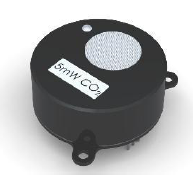
From the battery life point of view, the E2V IR11BD sensor seems the best option, but has serious drawbacks, such as the lack of an instrumentation amplifier (requiring its implementation in the node), so this part of the energy requirements is not evaluated. Also, the lack of double channel output means it needs continuous recalibrations. Based on considerations of energy, specifications and final sensor price, the CO2S-A model (SST Sensing Ltd., Coatbridge, UK) was chosen for the wireless node system. A view of this sensor is given in Figure 1.
3. Wireless CO2 Sensors Network
A wireless sensor network (WSN) consists of spatially distributed autonomous sensors to monitor physical or environmental conditions, such as temperature, sound, pressure, CO2, etc. and to pass the data acquired to a central personal computer (PC). As current networks are bi-directional, this means sensor activity can be controlled. Wireless sensor networks are now used in many industrial and consumer applications, such as industrial process monitoring, machine health monitoring, and so on.
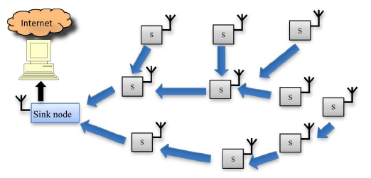
The WSN is built of “nodes”—which can vary in number from a few to several hundred or even thousands, in which each node is connected to one or several sensors. Each sensor network node is typically divided into several parts: a radio transceiver with an internal antenna or connection to an external antenna, a microcontroller, an electronic circuit for interfacing with the sensors and an energy source, usually a battery or an embedded form of energy harvesting. A sensor node can vary in size from that of a shoebox down to the size of a grain of dust, although functioning “motes” of genuine microscopic dimensions have yet to be created. The cost of sensor nodes is similarly variable, ranging from a few to hundreds of euros, depending on the complexity of the individual sensor nodes. Size and cost constraints on sensor nodes result in corresponding constraints on resources such as energy, memory, computational speed and communications bandwidth. The topology of the WSNs can vary from a simple star network to an advanced multi-hop wireless mesh network. The propagation technique between the hops of the network can be routing or flooding [18,20].
Figure 2 shows a typical scheme of a wireless sensor network. A set of nodes (S) transmits by a wireless protocol the information obtained through the network to the sink node. As can be seen in the Figure, some sensor nodes can act as repeaters, which allows low power transmit modes to be used to extend battery life. The sink node is connected by Universal Serial Bus (USB) or Ethernet to a personal computer to store the information received. Distance between sink nodes and nodes could be (using appropriate antennas and wireless technology) hundreds of meters.
3.1. System Architecture
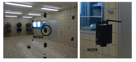
To demonstrate the feasibility of using a wireless sensor network to sense CO2 levels, 12 wireless nodes were implemented and installed in a controlled chamber (Figure 3).
The chamber is equipped with a set of fans that can reproduce air currents. As can be seen in Figure 3, the nodes were installed in the form of a matrix to measure the CO2 at different heights.
3.2. Node Characteristics
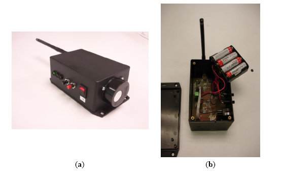
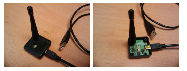
Figure 4 shows two views of the wireless CO2 node, which must be installed in a vertical arrangement to ensure that the CO2 sensor is below the node box. It allows airflow through the sensor and is protected from dust.
Figure 4a also shows three Light Emission Diodes (LED), two pushbuttons and the power on/off button. LEDs and pushbuttons are used basically to program the time between measures (sample and transmit frequency to the sink node). This time can be configured by pressing one of the buttons and selecting one of the following values: 15, 30, 60, 120, 300, 600, 1200 and 3600 s.
Figure 4b shows the node printed circuit board and the battery pack that ensures a measurement campaign of several weeks. Battery levels are monitored and sent to the sink node to warn users if a battery replacement is necessary.
The node is based on the CC1110F32 microcontroller (Texas Instruments, Dallas, TX, USA) [21]. The CC1110F32, is a true low-power sub-1 GHz system-on-chip designed for low power wireless applications. It combines the excellent performance of the state-of-the-art RF transceiver CC1101 with an industry-standard enhanced 8051 MCU, up to 32 KB of in-system programmable flash memory and up to 4 KB of Random Access Memory (RAM), and many other powerful features. The radio frequency range can be chosen from: 300–348 MHz, 391–464 MHz and 782–928 MHz. The European Industrial, Scientific and Medical (ISM) band 868 MHz frequency and 500 kbps were chosen for the present implementation. This ISM band allows longer ranges than typical systems using 2.4 GHz (up to almost 3 times higher for the same transmit power and sensitivity reception). Additionally, its low power demands (16 mA for transmission at 10 mW and 18 mA for reception) make it suitable for battery-powered systems. In our tests, ranges up to 290 m with an omnidirectional antenna were achieved, which was in excess of the requirements in livestock buildings.
The Sensirion SHT11 [22] digital humidity and temperature sensor was included to analyze the influence of temperature and humidity on CO2 measuring. This is the all-round version of the reflow solderable humidity sensor series that combines decent accuracy with a competitive price and is fully calibrated. The information transmitted to the sink node was as follows:
CO2 concentration
Ambient temperature
Relative humidity
Battery level
For the first three items, the node software averaged the last ten measures before sending the result to the sink node.
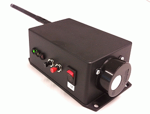
3.3. Sink Node
The sink node (see Figure 5) receives all the information transmitted by the set of nodes and communicates this data by means of a USB connection to a personal computer that stores all the information received in a Comma Separated Values (CSV) format file that can be processed by many standard PC applications (database or spreadsheet software).
The sink node hardware is the same as that of the other nodes, without the CO2 and temperature and humidity sensors. As it is connected by a USB port to the PC it does not need batteries. Although a USB connection was chosen for this system, other alternatives such as Ethernet connection or General Packet Radio Services (GPRS) can be implemented to send information to the PC.
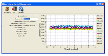
Figure 6 shows the user-friendly application used to store the acquired information in a CSV database.
3.4. Assessment of Sensor Performance
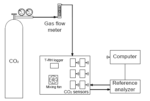
The next step consisted of the calibration and evaluation of sensors and a number of different tests under laboratory conditions to evaluate the performance of the wireless sensor network. The sensors were calibrated in a closed chamber measuring 50 cm long × 30 cm wide × 30 cm high lined with poly methylmethacrylate tiles under laboratory conditions. The chamber was equipped with a fan to homogenize the air inside it (Figure 7). Pure CO2 was injected into the chamber at a constant rate of 1 L per min until the target concentration was achieved. To reduce concentrations inside the chamber, fresh air was forced in at a constant rate of 2 L/min. The concentrations could be maintained inside the chamber when both flows were stopped. A photoacoustic gas analyzer (Innova 1412, LumaSense Technologies, Ballerup, Denmark) was used as a reference for CO2 concentration. This device has a precision of 1.5 ppm, which is considerably higher than the expected precision of the CO2 sensor network. Temperature and relative humidity were also measured by means of a data logger (HOBO U12-013, OnsetComp, Bourne, MA, USA). All these measurements were taken at a 1-min frequency, while the CO2 WSN registered information every 15 s. The different tests performed are described below.
Preliminary tests were conducted during sensor selection to evaluate linearity and potential interference under normal livestock-rearing conditions. Linearity was tested within the range from 500 to 5000 ppm by gradually varying gas concentration. Cross effects of temperature (16 °C, 24 °C and 32 °C) and relative humidity (15%, 40% and 60%) were assessed. As CH4 is normally present in livestock buildings as a result of fermentation processes it could potentially affect sensor readings as it also absorbs infrared radiation. Potential cross interference was evaluated by introducing this gas into the chamber from a calibration bottle (60% CH4–40% CO2) until 100 ppm were reached. The effect of the sensor node battery status was also monitored at values of 6.3 V (full battery), 5.7 V, 5.3 V and 4.9 V. An analysis of variance (ANOVA) was conducted to evaluate significant differences which could indicate cross interference by these factors.
As the preliminary tests showed that the sensor had a highly linear response to CO2 concentrations within the range from 500 to 5000 ppm, a three point calibration was conducted at approximately levels of 600, 2400 and 4000 ppm. The calibration consisted of placing all the sensors inside the chamber and injecting CO2 as described above until a constant value was reached by both the reference analyzer and the sensors under study. Once equilibrium was reached, each level was maintained for 30 min. All the tests were conducted at 24 °C ambient temperature and 50% relative humidity. The full procedure was repeated four times.
The calibration curve for each sensor was obtained by simple regression using the measurements for each sensor as a dependent variable and the corresponding measurements of the reference analyzer as independent variable. Homogeneity between the sensors was tested using a multiple regression which included sensor influence on intercept and slope as dummy variables, according to the following model:
From this test sensor precision was also obtained at the different CO2 levels tested for calibration (600, 2400 and 4000 ppm). Following ISO 3534-2:2006 [23], precision was defined as the standard deviation of concentrations given by the sensor (after applying the calibration curve). According to this standard, this represents repeatability, i.e., the precision under observation conditions in which independent results are obtained by the same method on identical measurement items in the same test by the same operator and equipment within short intervals of time.
The time response of the sensor to a sharp decrease in ambient CO2 concentration was also studied. Sensors were maintained for 30 min inside the chamber at a constant CO2 concentration of about 5000 ppm. After this period, they were removed from the chamber and exposed to fresh air (CO2 concentration about 400 ppm) in still air (air velocity = 0 m/s), after which sensor readings were taken for another 30 min. Temperature and relative humidity did not show relevant changes (less than 0.2 °C and less than 1%, respectively) between both sensor positions (inside and outside the chamber).This procedure was repeated 9 times. According to the preliminary tests, 30 min was enough for the sensor to stabilize. During this changeover period, the sensor signal followed a decay curve according to the following general equation:
Once k had been obtained, the average times needed to achieve a 90% and 95% change in readings were determined.
4. Results and Discussion
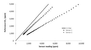
Preliminary tests on two sensors demonstrated that the sensor was highly linear within the range from 500 to 5000 ppm, which includes most practical situations in livestock operations (Figure 8). In all the tests a very good linear response (R2 > 0.99) was obtained from the sensor. However, these preliminary tests also revealed very relevant differences among sensor performance (see different slopes for sensors 1 and 2 in Figure 8).
Regarding potential cross effects, temperature, relative humidity and battery status did not have any effect on CO2 readings at the studied levels (p > 0.05). However, exposure to 100 ppm of CH4 caused a sensor underestimation of about 10% in CO2 readings. This gas may accumulate in livestock buildings, particularly in ruminant houses and manure storage facilities. Although in poultry production CH4 concentrations are typically lower than 10 ppm [14,16], in dairy cow barns it may be as high as 40 ppm [24]. Specific research should be conducted to determine with precision how exposure to different levels of CH4 affects NDIR CO2 sensor readings under practical farm conditions.
Calibration tests of all 12 sensors indicated varying responses of individual sensors to the same CO2 concentrations (Table 3). Significant differences were noted between all the sensors, which suggests the need for individual calibration. On the other hand, temperature and relative humidity readings showed only non-significant differences. The temperature differences were always less than 0.4 °C, whereas for relative humidity the differences consistently lower than 1.5%.
Sensor calibration parameters are indicated in Table 4. As suggested by the results in Table 3, calibration curves were statistically different between sensors (p < 0.05), which meant a specific calibration equation was required for each sensor. As in the preliminary results, all the calibrations showed a very good linear relationship (R2 was consistently over 0.99). The standard error of estimation (SEE) obtained by the regression model is an estimation of sensor precision and represents the deviations of sensor readings in comparison with reference values. As indicated above, this value represents sensor repeatability. Sensor precision ranged from 58.2 ppm (Sensor #1) to 117 ppm (Sensor #11), most of the sensors being within the 80 to 110 ppm range.
One of the most positive sensor characteristics is its very high linearity, which allows two- or three-point calibration. However, the response was found to vary significantly from one sensor to another, so that individual calibrations were required. Sensor precision measured under laboratory conditions was about 2 times the catalog value (50 ppm).
Field experiments should be conducted to determine whether this precision is maintained under non-controlled conditions. This degree of precision may be enough for welfare assessment, when 3000 to 5000 ppm are established as threshold values. This sensor may also be sufficiently reliable to implement climate control systems using CO2 as a ventilation criterion. In such systems, ventilation comes into operation when CO2 exceeds a specific value (e.g., 3000 ppm in broiler houses, according to European Council Directive 2007/43/EC) [11].
However, these sensors could also be used to conduct CO2 balances to indirectly estimate ventilation flows under certain conditions. As indicated by Ouwerkerk and Pedersen in [13], the CO2 measurement system should be accurate enough to detect differences of at least 150 ppm between air outlets and inlets. In practice, CO2 balances are easier to conduct when the difference in concentration is higher, as in enclosed animal buildings, which normally have well defined air inlets and outlets. However, the great potential of CO2 balances may be associated with relatively open buildings, in which CO2 differences may be lower than 150 ppm and which may even be subject to incomplete mixing of fresh and polluted air. For example, [16,17] reported buildings with average CO2 concentrations lower than 500 ppm in pig and poultry houses, whereas [25] reported an average concentration of 553 ppm in a dairy cow house, where indoor CO2 concentrations as low as 313 ppm (similar to outdoor concentration) were measured. Similar results were reported by [24]. Unfortunately, this sensor may not be accurate enough in such cases.
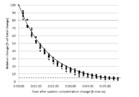
The sensor response time is shown in Figure 9, which represents the decrease in concentration expressed in relative terms, from 100% (initial concentration) to 0% (final or equilibrium concentration) when concentrations suddenly change from high to low. The time necessary to achieve a specific change of concentration can be obtained from this curve. According to Equation (3), a decay constant k = 0.582 min−1 was obtained. Following this model, it was determined that a 90% change in concentration is obtained in 3 min and 57 s, whereas a 95% change is obtained in 5 min and 8 s. According to the curves shown in Figure 9, it can be concluded that this behavior was constant for all the sensors.
A similar response time to that obtained in the present study was also obtained in [19], whose authors tested five different NDIR CO2 sensors and obtained 90% response times varying from less than 1 min to 3 min and 10 s, which is considerably lower than the time response of the SST CO2S-A sensor used in this study. The sensor response obtained by us is adequate for questions of animal welfare, considering that indoor CO2 concentrations are relatively constant in most livestock buildings. It can also be considered acceptable for characterizing the indoor climate and measuring emissions in most mechanically-ventilated livestock buildings, in which air fluxes tend to be stable. However, this response is too slow to determine CO2 fluxes in naturally ventilated buildings. These buildings are characterized by variable and unpredictable changes in flow directions, in such a way that air inlets and outlets may change in short time intervals as a consequence of turbulence and changes in outdoor conditions. For this reason, the boundary conditions of these buildings normally involve sudden changes in CO2 concentrations, from relatively high (when an opening is acting as an air outlet) to low, background CO2 concentrations (when air is entering).
As reported in [19], the output of NDIR sensors is affected by the length of time they are in use. They found a linear relationship in sensor response as a function of time when used for less than one year, which may be considered correct sensor output. Although this effect was not analyzed in our study, preliminary information suggests that this effect may also occur with the sensors we used. In this sense, some significant differences can be found in calibration curves separated in time more than one week. Therefore, must be conducted to evaluate the long-term performance of these sensors. Frequent sensor calibrations would thus be advisable before use. Response time could also be affected by the length of time in use. Although [19] did not find any clear relationship between these two variables, it must be considered that sensor response is affected by gas diffusion through a membrane to the sensor chamber, so that the factors affecting membrane permeability (e.g., dust accumulation) may slow down the sensor response. According to [26,27], in these sensors there is a potential cross interference with dust due to light scattering and therefore sensors are placed in closed or diffusion cells protected by dust filters. For this reason, dust accumulation in these filters may reduce diffusion to the measurement cell, thus affecting response time of these NDIR sensors
5. Conclusions
This paper describes a study on the use of a low cost CO2 sensor implemented in a wireless sensor network system that showed an excellent throughput during measurement campaigns. This system combines moderate cost with low energy requirements and can be powered by standard batteries, which simplifies its installation. A set of nodes can be placed at different points throughout a livestock building to acquire readings. The nodes are also designed to make it possible to include other CO2 sensors or additional sensors to detect the presence of other gases (i.e., methane).
The CO2 sensor selected may be appropriate for animal welfare and environmental applications in livestock production, particularly in animal houses which are relatively open to the atmosphere. The sensors were seen to respond linearly to changes in CO2 concentrations. However, the differences between individual sensors and a potential time drift make it advisable to calibrate before a measurement campaign. The sensor time response (about 5 min) makes it appropriate for most applications, except those requiring a fast response. For this reason these sensors may not be appropriate to monitor slight, sudden changes occurring in open, naturally ventilated buildings.
Acknowledgments
This project was supported by the Vicerrectorado de Investigación of the UPV (Programa de Apoyo a la Investigación y Desarrollo, PAID-06-11 Program, Project No. 2843) and the Spanish Government under Projects CTM2011-29691-C02-01 and TIN2011-28435-C03-0. The translation of this paper was funded by the Universitat Politècnica de València, Valencia, Spain.
Author Contributions
Salvador Calvet coordinated the calibration tests and wrote the corresponding part of the manuscript. José Carlos Campelo and Angel Perles selected the set of CO2 sensors and developed the firmware for the wireless sensor network and write the related parts of this paper. Ricardo Mercado designed the hardware subsystem. Fernando Estellés performed sensor calibrations. Juan José Serrano designed the wireless sensor network.
Conflicts of Interest
The authors declare no conflict of interest.
References
- Wathes, C.M.; Jones, J.B.; Kristensen, H.H.; Jones, E.K.M.; Webster, A.J.F. A version of pigs and domestic fowl to atmospheric ammonia. Trans. ASAE 2002, 45, 1605–1610. [Google Scholar]
- Homidan, A.A.; Robertson, J.F.; Petchey, A.M. Review of the effect of ammonia and dust concentrations on broiler performance. Worlds Poult. Sci. J. 2003, 59, 340–349. [Google Scholar]
- Krupa, S.V. Effects of atmospheric ammonia (NH3) on terrestrial vegetation: A review. Environ. Pollut. 2003, 124, 179–221. [Google Scholar]
- IPCC Fourth Assessment Report of the Intergovernmental Panel on Climate Change; Intergovernmental Panel on Climate Change (IPCC): Geneva, Switzerland, 2007; pp. 1–74.
- 2006 IPCC Guidelines for Greenhouse Gas Inventories, Prepared by the National Greenhouse Gas Inventories Programme; Intergovernmental Panel on Climate Change (IPCC): Geneva, Switzerland, 2006.
- 4th Report of Working Group on Climatization of Animal Houses: Heat and Moisture Production at Animal and House Levels; Research Centre Bygholm, Danish Institute of Agricultural Sciences: Horsens, Denmark, 2002.
- Kaye, J.; Buchanan, J.; Kendrick, A.; Johnson, P.; Lowry, C.; Bailey, J.; Nutt, D.; Lightman, D. Acute carbon dioxide exposure in healthy adults: Evaluation of a novel means of investigating the stress response. J. Neuroendocrinol. 2004, 16, 256–264. [Google Scholar]
- Ni, J.Q.; Heber, A.J. Sampling and measurement of ammonia at animal facilities. Adv. Agron. 2008, 98, 201–269. [Google Scholar]
- Ogink, N.W.M.; Mosquera, J.; Calvet, S.; Zhang, G. Methods for measuring gas emissions from naturally ventilated livestock buildings: Developments over the last decade and perspectives for improvement. Biosyst. Eng. 2013, 116, 297–308. [Google Scholar]
- Calvet, S.; Gates, R.S.; Zhang, G.; Estellés, F.; Ogink, N.W.M.; Pedersen, S.; Berckmans, D. Measuring gas emissions from livestock buildings: A review on uncertainty analysis and error sources. Biosyst. Eng. 2013, 116, 221–231. [Google Scholar]
- Council directive 2007/43/EC laying down minimum rules for the protection of chickens kept for meat production. Off. J. Eur. Union 2007, L182, 19–28.
- Phillips, V.R.; Holden, M.R.; Sneath, R.W.; Short, J.L.; White, R.P.; Hartung, J.; Seedorf, J.; Schroder, M.; Linkert, K.H.; Pedersen, S.; et al. The development of robust methods for measuring concentrations and emission rates of gaseous and particulate air pollutants in livestock buildings. J. Agric. Eng. Res. 1998, 70, 11–24. [Google Scholar]
- Van Ouwerkerk, E.N.J.; Pedersen, S. Application of the carbon dioxide mass balance method to evaluate ventilation rates in livestock buildings. Proceedings of the XII World Congress on Agricultural Engineering, Milan, Italy, 29 August–1 September 1994; pp. 516–529.
- Calvet, S.; Cambra-Lopez, M.; Estelles, F.; Torres, A.G. Characterization of gas emissions from a Mediterranean broiler farm. Poult. Sci. 2011, 90, 534–542. [Google Scholar]
- Calvet, S.; Cambra-Lopez, M.; Estelles, F.; Torres, A.G. Characterization of the indoor environment and gas emissions in rabbit farms. World Rabbit Sci. 2011, 19, 49–61. [Google Scholar]
- Wathes, C.M.; Holden, M.R.; Sneath, R.W.; White, R.P.; Phillips, V.R. Concentrations and emission rates of aerial ammonia, nitrous oxide, methane, carbon dioxide, dust and endotoxin in UK broiler and layer houses. Br. Poult. Sci. 1997, 38, 14–28. [Google Scholar]
- Pedersen, S.; Takai, H.; Johnsen, J.O.; Metz, J.H.M.; Groot Koerkamp, P.W.G.; Uenk, G.H.; Phillips, V.R.; Holden, M.R.; Sneath, R.W.; Short, J.L.; et al. A comparison of three balance methods for calculating ventilation rates in livestock buildings. J. Agric. Eng. Res. 1998, 70, 25–37. [Google Scholar]
- Dargie, W.; Poellabauer, C. Fundamentals of Wireless Sensor Networks: Theory and Practice; John Wiley and Sons: New York, NY, USA, 2010. [Google Scholar]
- Yasuda, T.; Yonemura, S.; Tani, A. Comparison of the characteristics of small commercial NDIR CO2 sensor models and development of a portable CO2 measurement device. Sensors 2012, 12, 3641–3655. [Google Scholar]
- Sohraby, K.; Minoli, D.; Znati, T. Wireless Sensor Networks: Technology, Protocols, and Applications; John Wiley and Sons: New York, NY, USA, 2007. [Google Scholar]
- Texas Instruments. CC1110F32. Low-Power SoC (System-on-Chip) with MCU, Memory, Sub-1 GHz RF Transceiver, and USB Controller. Available online: www.ti.com/product/cc1110f32 (accessed on 9 June 2014).
- Sensirion. SHT11: Digital Humidity Sensor (RH&T). Available online: http://www.sensirion.com/en/products/humidity-temperature/humidity-sensor-sht11/ (accessed on 9 June 2014).
- Statistics—Vocabulary and symbols—Part 2: Applied Statistics; ISO 3534-2:2006; International Organization for Standardization (ISO): Geneva, Switzerland, 2006.
- Bjerg, B.; Zhang, G.; Madsen, J.; Rom, H.B. Methane emission from naturally ventilated livestock buildings can be determined from gas concentration measurements. Environ. Monit. Assess. 2012, 184, 5989–6000. [Google Scholar]
- Kaasik, A.; Maasikmets, M. Concentrations of airborne particulate matter, ammonia and carbon dioxide in large scale uninsulated loose housing cowsheds in Estonia. Biosyst. Eng. 2013, 114, 223–231. [Google Scholar]
- Hodgkinsona, J.; Smith, R; On Ho, W.; Saffell, J.R.; Tatama, R.P. Non-dispersive infra-red (NDIR) measurement of carbon dioxide at 4.2 μm in a compact and optically efficient sensor. Sens. Actuators B 2013, 186, 580–588. [Google Scholar]
- Zosel, J.; Oelßner, W.; Decker, M.; Gerlach, G.; Guth, U. The measurement of dissolved and gaseous carbon dioxide concentration. Meas. Sci. Technol. 2011, 22. [Google Scholar] [CrossRef]


| Manufacturer | Hanwei | SST Sensing | Alphasense | Dynament | E2V | Senseair |
|---|---|---|---|---|---|---|
| Model | MH-Z12 | CO2S-A | IRC-A1 | TDS0037 | IR11BD | K30 |
| Measurement range (ppm) | 0–5,000 | 0–5,000 | 0–5,000 | variable | variable | 0–10,000 |
| Accuracy | ±50 ppm | ±50ppm ±3% measure | 1% | 2% | ±100 ppm | ±30ppm ±5% measure |
| Response time (s) | <30 + 180 preheat | 30 to 180 | <40 | < 30 + 60 preheat | < 20 + 30 to 1800 preheat | 20 |
| Operating voltage (V) | 4–6 | 3.25–5 | 2–5 | 3–5 | 3–15 | 4.5–14 |
| Size (mm) (Height × height × depth /Ø Diameter × height) | 60 × 42 × 15 | Ø 60 × 20 | Ø 20 × 17 | Ø 20 × 17 | Ø 14 × 19 | 51 × 51 × 41 |
| Approximate price (Euros) | 120 | 80 | 75 | 100 | 150 | 70 |
| Measure interval (min) | Model | |||||
|---|---|---|---|---|---|---|
| Hanwei MH-Z12 | SST Sensing CO2S-A | Alphasense IRC-A1 | Dynament TDS0037 | E2V IR11BD | Senseair K30 | |
| Cont. | 1.2 | 3.6 | 1.2 | 0.9 | 2 | 1.8 |
| 5 | 1.7 | 7.2 | 5.1 | 3.0 | 15.0 | 6.0 |
| 10 | 3.4 | 14.4 | 10.3 | 6.0 | 30.0 | 12.0 |
| 15 | 5.1 | 21.6 | 15.4 | 9.0 | 45.0 | 18.0 |
| 20 | 6.9 | 28.8 | 20.6 | 12.0 | 60.0 | 24.0 |
| 25 | 8.6 | 36.0 | 25.7 | 15.0 | 75.0 | 30.0 |
| 30 | 10.3 | 43.2 | 30.9 | 18.0 | 90.0 | 36.0 |
| 120 | 41.1 | 172.8 | 123.4 | 72.0 | 360.0 | 144.0 |
| 360 | 123.4 | 518.4 | 370.3 | 216.0 | 1080.0 | 432.0 |
| CO2 level | 600 | 2400 | 4000 |
|---|---|---|---|
| Reference | 607.9 ± 2.0 | 2386.5 ± 2.1 | 4039.4 ± 4.3 |
| Sensor #1 | 2328.0 ± 2.1 | 5823.5 ± 4.0 | 9153.7 ± 6.9 |
| Sensor #2 | 841.6 ± 2.1 | 3013.3 ± 4.0 | 5073.8 ± 6.3 |
| Sensor #3 | 774.1 ± 2.1 | 2843.2 ± 4.0 | 4885.5 ± 6.3 |
| Sensor #4 | 1976.8 ± 2.1 | 5133.0 ± 4.0 | 8280.0 ± 6.3 |
| Sensor #5 | 943.2 ± 2.1 | 3150.3 ± 4.0 | 5339.7 ± 6.3 |
| Sensor #6 | 743.1 ± 2.1 | 2751.7 ± 4.0 | 4762.0 ± 6.3 |
| Sensor #7 | 866.6 ± 2.1 | 2992.8 ± 4.0 | 5111.2 ± 6.3 |
| Sensor #8 | 828.0 ± 2.1 | 2951.6 ± 4.0 | 5079.9 ± 6.3 |
| Sensor #9 | 978.7 ± 2.1 | 3164.2 ± 4.0 | 5274.7 ± 6.3 |
| Sensor #10 | 1219.9 ± 2.1 | 3547.7 ± 4.0 | 5759.0 ± 6.3 |
| Sensor #11 | 1333.6 ± 2.1 | 3779.1 ± 4.0 | 6132.3 ± 6.3 |
| Sensor #12 | 822.0 ± 2.1 | 2921.5 ± 4.0 | 4993.7 ± 6.3 |
| CO2 level | β0 | β1 | R2 | SEE (ppm) |
|---|---|---|---|---|
| Sensor #1 | −537.4 (3.6) | 0.498 (0.0006) | 0.998 | 58.2 |
| Sensor #2 | −60.46 (3.9) | 0.808 (0.001) | 0.997 | 74.8 |
| Sensor #3 | −6.6 (4.7) | 0.829 (0.001) | 0.996 | 91.5 |
| Sensor #4 | −438.3 (4.6) | 0.543 (0.001) | 0.997 | 80.3 |
| Sensor #5 | −88.7 (5.7) | 0.774 (0.002) | 0.994 | 109.0 |
| Sensor #6 | 7.2 (4.6) | 0.849 (0.001) | 0.996 | 91.0 |
| Sensor #7 | −57.2 (4.5) | 0.803 (0.001) | 0.996 | 87.5 |
| Sensor #8 | −24.5 (4.3) | 0.802 (0.001) | 0.997 | 83.3 |
| Sensor #9 | −144.9 (5.5) | 0.793 (0.001) | 0.995 | 102.3 |
| Sensor #10 | −283.9 (6.1) | 0.749 (0.002) | 0.994 | 110.5 |
| Sensor #11 | −309.0 (6.6) | 0.708 (0.002) | 0.993 | 117.1 |
| Sensor #12 | −37.0 (4.5) | 0.818 (0.001) | 0.996 | 86.6 |
© 2014 by the authors; licensee MDPI, Basel, Switzerland. This article is an open access article distributed under the terms and conditions of the Creative Commons Attribution license ( http://creativecommons.org/licenses/by/3.0/).
Share and Cite
Calvet, S.; Campelo, J.C.; Estellés, F.; Perles, A.; Mercado, R.; Serrano, J.J. Suitability Evaluation of Multipoint Simultaneous CO2 Sampling Wireless Sensors for Livestock Buildings. Sensors 2014, 14, 10479-10496. https://doi.org/10.3390/s140610479
Calvet S, Campelo JC, Estellés F, Perles A, Mercado R, Serrano JJ. Suitability Evaluation of Multipoint Simultaneous CO2 Sampling Wireless Sensors for Livestock Buildings. Sensors. 2014; 14(6):10479-10496. https://doi.org/10.3390/s140610479
Chicago/Turabian StyleCalvet, Salvador, José Carlos Campelo, Fernando Estellés, Angel Perles, Ricardo Mercado, and Juan José Serrano. 2014. "Suitability Evaluation of Multipoint Simultaneous CO2 Sampling Wireless Sensors for Livestock Buildings" Sensors 14, no. 6: 10479-10496. https://doi.org/10.3390/s140610479