Self-Configuring Indoor Localization Based on Low-Cost Ultrasonic Range Sensors

Abstract
: In smart environments, target tracking is an essential service used by numerous applications from activity recognition to personalized infotaintment. The target tracking relies on sensors with known locations to estimate and keep track of the path taken by the target, and hence, it is crucial to have an accurate map of such sensors. However, the need for manually entering their locations after deployment and expecting them to remain fixed, significantly limits the usability of target tracking. To remedy this drawback, we present a self-configuring and device-free localization protocol based on genetic algorithms that autonomously identifies the geographic topology of a network of ultrasonic range sensors as well as automatically detects any change in the established network structure in less than a minute and generates a new map within seconds. The proposed protocol significantly reduces hardware and deployment costs thanks to the use of low-cost off-the-shelf sensors with no manual configuration. Experiments on two real testbeds of different sizes show that the proposed protocol achieves an error of 7.16∼17.53 cm in topology mapping, while also tracking a mobile target with an average error of 11.71∼18.43 cm and detecting displacements of 1.41∼3.16 m in approximately 30 s.1. Introduction
Target tracking is a process of continuously recording the locations of a target, e.g., a human, in time. In smart environments, this is an essential service because most of the user interactions are through location-aware activities [1]. Health-care systems report the location of a user to medical professionals in the event of an emergency; activity recognition systems use the rooms that a user has occupied and the objects s/he has used at a certain point of time in order to infer the context; and infotainment systems use similar information to provide a user with personal feeds as s/he moves inside the environment. These interaction models, tightly coupled with location awareness, mean that the smart space experience is shaped by the existence and accuracy of a target tracking system.
Target tracking solutions can be broadly categorized into either intrusive or non-intrusive systems. The former uses a dedicated device (target) carried by a user to send messages, e.g., Wi-Fi signals, to the system, while the latter or a device-free system tries to solve the problem without relying on such a device [2]. The identity of a user is readily available in the intrusive system since this device can contain a unique identifier. By contrast, in the non-intrusive system, a user is identified by analyzing sensor readings such as weight and/or height measurements, or by face recognition at certain checkpoints in the environment [3]. Once the user is identified, the system may start sampling the location of the user regularly in order to construct a track.
Whether intrusive or not, the target should be located based on its distance to some reference points that have known locations. Therefore, the system also needs to preconfigure or determine the locations of the reference points, i.e., landmarks; this process can be rehashed into a sensor localization problem that determines relative or absolute locations of sensor nodes in a sensor network [4]. However, the problem is not trivial when applied to the smart environments since GPS devices cannot be used indoors and also the walls and furniture cause interference and multipath effects, hindering the accuracy of distance measurements [5]. Moreover, smart home sensor localization solutions [6–8] generally depend on manual mapping of landmarks, but manually defining their locations is undesirable as it complicates the deployment and makes the system fragile. For example, if somehow one sensor is displaced after mapping, the system will fail to operate and will require manual reconfiguration.
Motivated by these limitations, we aim to design the tracking system to work out of the box as illustrated in the following deployment scenario. A user simply ‘puts’ sensors at convenient locations and turns them on. Then the sensors cooperatively pass through a self-configuration phase, in which they collect data on users’ movements across their field-of-view for a short period of time and transform themselves into landmarks for target tracking by having their relative locations calculated and memorized. The system then switches to a tracking phase, in which the landmarks calculate the locations of users in real-time as well as monitor their surroundings to detect any sensor displacements and fix the sensor topology if detecting changes.
To realize this scenario, we propose a self-configuring and low-cost localization protocol for smart environments using cheap off-the-shelf distance sensors such as ultrasonic rangers [9]. The proposed protocol is capable of facilitating device-free indoor tracking of users with zero prior knowledge of the geographic topology while also allowing hassle-free deployment without the need for manual configuration. As opposed to traditional localization protocols that rely on estimated distances between sensor nodes, the proposed protocol works on concurrent distance measurements to a mobile target or a user. The key idea of the proposed protocol is to exploit the mobility of the user for accurate localization and tracking. To do so, our protocol applies a Genetic Algorithm (GA) for identifying the locations of sensors on a 2-dimensional space, which yields sufficiently accurate results compared to outdoor environments. The located sensors are then used as landmarks for indoor target tracking. Moreover, our protocol effectively handles the events of sensor displacement, which is common in our user-friendly deployment scenario, by employing a lightweight scheme for detecting such events in real time and recovering from changes to sensor locations. Our experiments on two real testbeds of different sizes, i.e., 2 × 3 m2 and 4 × 6 m2, indicate that the proposed protocol can achieve an error of 7.16 to 17.53 cm in identifying landmark locations while also tracking a mobile target with an average error of 11.71 to 18.43 cm. Moreover, we observe the proposed protocol is capable of detecting and handling displacements of magnitude, 1.41∼3.16 m in approximately 30 s.
The rest of the paper is organized as follows. In Section 2 we go over the literature and give a brief summary of the related work. In Section 3 we briefly go over the sensor hardware used in our implementation and discuss its limitations. In Sections 4 and 5, we describe our self-configuring localization and tracking algorithms in details. Based on the need for easy deployment of sensing infrastructure, we design a self-configuring, device-free, and cost-effective localization protocol that uses distance measurements to the target for accurate localization among landmark sensors, and further extend the protocol to automatically identify the displacement of landmarks by reusing the localization algorithm. We further develop a heuristic-based target tracking system based on the genetic algorithm by employing the thus-designed self-configuring protocol, and show that our system is robust to measurement errors in contrast to the existing algorithms, e.g., those based on mathematical formulations, because it finds the best solution that fits the measurements. In Section 6 we present the experimental setup and provide results of comprehensive experiments conducted on the real testbed. We demonstrate that the protocol significantly reduces the system complexity and deployment cost as well as achieves high level of accuracy in tracking targets over a broad range of network layouts. Finally, we discuss possible future directions and conclude this paper in Section 7.
2. Related Work
Device-aided indoor tracking systems benefit from GPS devices, cell phones, or RFID tags [10–13]. For instance, the algorithm in [14] describes an anchor-free indoor localization technique based on the strength of Wi-Fi signals. However, this algorithm relies on infrequent GPS checkpoints and requires users to carry a Wi-Fi receiver. These systems typically use collaborating devices carried by the users, and may be most suitable for in-building localization/tracking systems, while in a smart home environment devices create significant inconvenience for the users. A method for locating humans within a room using cameras has been proposed, but using cameras is undesirable in a smart home environment due to privacy issues [15]. This is especially true for bedrooms and bathrooms where people feel an invasion of privacy in the presence of visual sensors. SCPL is a device-free tracking system which uses radio signals to track multiple people [16]. However, the system requires a known floor plan of the environment and this considerably complicates the deployment process.
The use of GA for sensor network localization is not novel by itself. In fact, localization is an interesting application of GA as shown in [8,17–20]. One of the previous GA-based algorithms, GA-Loc assumes that distances between one-hop neighbors are known and tries to minimize the difference between measured distances and those that are obtained by the estimated locations [19]. While this algorithm does not necessitate nodes with known locations, it uses inter-node distances and obtaining this information indoors requires complex hardware. Mark et al. [21] introduced a two-phase GA-based algorithm using distances between one-hop neighbors. The first phase calculates locations of nodes that have three immediate anchor neighbors via trilateration. The second phase includes all other nodes and uses GA to minimize difference between known and estimated distances between nodes. The work on the use of GA-based systems in target tracking is scarce in the literature. The main focus of existing work is associating sensor readings with targets in multi-target tracking systems [22,23]. However, our proposed system does not focus on multi-target tracking.
While none of these algorithms cannot simultaneously meet the requirements of anchor-free, device-free, low-cost, and high-accuracy localization, our proposed algorithm successfully addresses these requirements by associating GA with human mobility.
3. Sensor Hardware and Related Challenges
3.1. Sensor Hardware
We aim to realize a cost-effective localization solution by using off-the-shelf ultrasonic ping sensors for distance measurement [2,24]. A ping sensor, having a transducer and a receiver, measures the distance to an object by emitting a short ultrasonic 40 kHz burst and then calculating the time difference of arrival (TDOA) of the reflected wave with respect to the original burst. Since the echo is reflected from the object of interest, the distance can be calculated by considering the speed of sound and the TDOA. Note that the speed of sound is affected by both temperature and humidity. While the latter (humidity) does not significantly impact the sound propagation in environments with normal air pressure, the former (temperature) must be considered in calculating the speed of sound [25,26]. This sensor has a 40° beam angle, and can sense objects within a range of 2∼300 cm. One issue with this type of sensors is how to determine if the reflecting surface is a part of the environment such as a wall or furniture, or a mobile target. Another problem is their vulnerability to interference from other ultrasonic sources; for instance, the receiver of one sensor may sense the signal from the transducer of another sensor when concurrent readings are taken from different sensors. A similar problem occurs if a sensor picks up an echo of a previous signal still residing in the room. In such cases the readings are meaningless and should be discarded. One way to prevent these problems is to introduce a delay, ε, between subsequent sensor readings [9]. In our implementation, two measurements are at least 0.2 s apart, i.e., ∊ = 0.2.
3.2. Formation of Input Database
The distance measurements are accumulated in the input database
 , in which each entry dtk is the distance of the target to sensor k at time t where k = 1, ⋯, K. Note that a typical value of K is 4. We define a row dt = {dt1 ⋯ dtK} of
to be a problem instance. If an actual geographic map of sensors is already known, we can use three valid (i.e., noise-free) elements in dt to calculate the location of the target at time t using trilateration [27]. Solving a problem instance to get the location requires that all elements in dt are measurements to the same reference point. However, since we consider a mobile target as the point of reference, the sensing delay ε between consecutive measurements becomes a major source of error. In case the mobile target moves between two measurements during the construction of dt, the assumption of having a common reference point across dt breaks. Furthermore, as the number of elements in dt, i.e., |dt|, increases, the problem gets worse since the maximum time difference between any pair of measurements can be as large as ∊ × (|dt| − 1) and a possible shift in the position of the reference point between measurements in dt can be significant. Another source of error is the inaccuracy of distance measurements. Although ultrasonic sensors have an error range less then ±5 cm, the method of measurement is vulnerable to multipath effects as explained earlier.
, in which each entry dtk is the distance of the target to sensor k at time t where k = 1, ⋯, K. Note that a typical value of K is 4. We define a row dt = {dt1 ⋯ dtK} of
to be a problem instance. If an actual geographic map of sensors is already known, we can use three valid (i.e., noise-free) elements in dt to calculate the location of the target at time t using trilateration [27]. Solving a problem instance to get the location requires that all elements in dt are measurements to the same reference point. However, since we consider a mobile target as the point of reference, the sensing delay ε between consecutive measurements becomes a major source of error. In case the mobile target moves between two measurements during the construction of dt, the assumption of having a common reference point across dt breaks. Furthermore, as the number of elements in dt, i.e., |dt|, increases, the problem gets worse since the maximum time difference between any pair of measurements can be as large as ∊ × (|dt| − 1) and a possible shift in the position of the reference point between measurements in dt can be significant. Another source of error is the inaccuracy of distance measurements. Although ultrasonic sensors have an error range less then ±5 cm, the method of measurement is vulnerable to multipath effects as explained earlier.
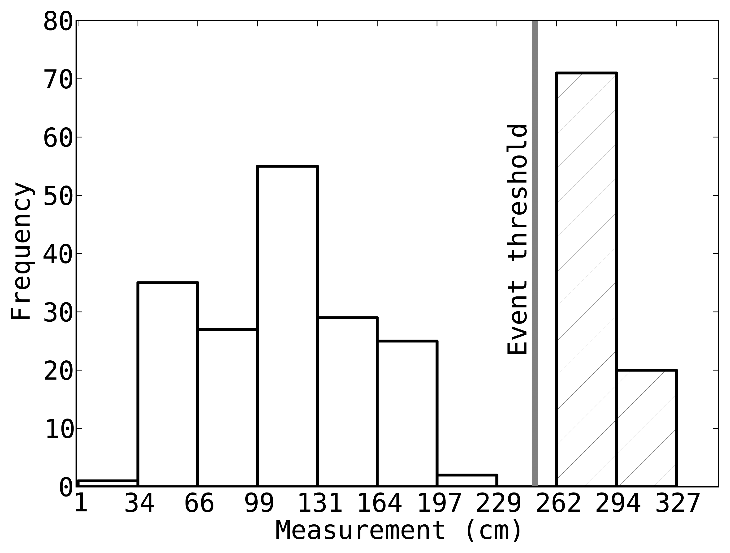
To deal with the above difficulties, we use a two-step approach to remove noise from
: The first step erases non-event measurements (outliers) while the second step filters out low-quality measurements. When the mobile target enters into the line-of-sight, meaning that an event occurs, the sensor records a smaller TDOA value compared to the samples taken when the field-of-view is clear [2]. The first step exploits this property and analyzes the sensor readings by setting an event threshold to 60% of the readings. Hence, a reading less then this event threshold fires an event and is inserted into
, otherwise, the element corresponding to this sensor is marked as invalid. Figure 1 shows the event threshold for one of the sensors in our testbed along with the histogram of measurements recorded by that sensor. We note this simple method removes more than 99% of the non-event data from
across all sensors.
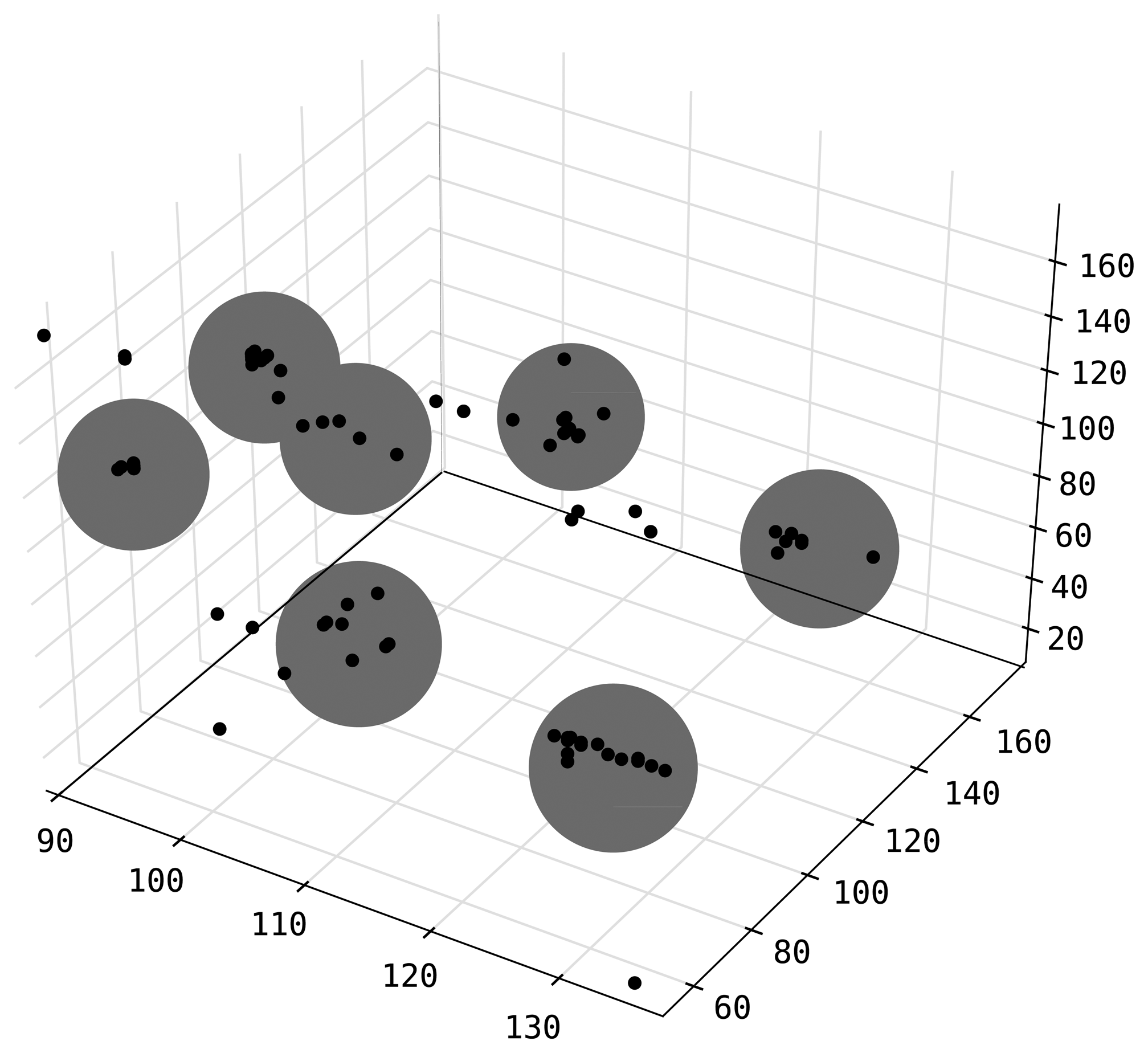
In the second step of noise removal, the rows of
are clustered using a DBSCAN algorithm [28]. Interpreting dt as the K-dimensional coordinates of a target, DBSCAN clusters together rows that are in 10 cm proximity of each other in this K-dimensional space. Any cluster with less than 10 members is discarded. After this step, we can make sure that each row in
is an accurate observation of the same target. An example clustering result for measurements from 3 sensors is given in Figure 2 where dark points are readings and gray large dots mark cluster boundaries. We tested this filtering mechanism by collecting distance measurements to predetermined checkpoints while visiting the checkpoints regularly in an otherwise random walk fashion. We verified the system can identify outlier observations and filter them out.
Although clustering on 10 cm neighborhood, and using 10 members as the density threshold may seem arbitrary, the fixed sensing range and error characteristics of the hardware make this configuration generally applicable. This approach also handles errors due to the mobility of the target because clustered rows of
correspond to events in which the target is slow or stationary.
4. Self-Configuring Localization for Landmarks
In this section, we present a GA-based algorithm, called Self-configuring Localization for Landmarks (SeLL), to determine initially unknown locations of ultrasonic range sensors that will serve as landmarks for target tracking. SeLL works on a cluster of K sensors. Given an input database
of distances, SeLL tries to find the actual locations of K sensors, L = {l1, l2, …, lK} by exploiting the movement of mobile target. As mentioned earlier, each row dt of
is a set of measurements to the same reference point obtained by K sensors. In fact these reference points associated with rows of
are snapshots of the mobile target’s trajectory. SeLL thus searches for a set of feasible locations, L̂ = {l̂1, l̂2, …, l̂K} that would yield a solution for each and every reference point in
, based on the assumption that a solution for all of the reference points can be found if and only if L = L̂. Once the relative locations of sensors in each cluster is found, these clusters are aggregated into a complete topology that includes all of the sensors in the environment.
As shown in Algorithm 1, SeLL starts with a set of z randomly generated estimations, G = {L̂1, … , L̂z}. In GA terms, G is the population and each L̂i = {l̂i1, l̂i2, …, l̂ik} is an individual that estimates the locations of sensors where l̂ik = {x̂ik, ŷik} is a point on a 2-dimensional plane representing the location of sensor k in L̂t. To calculate the location of the reference point based on L̂i, let us define Cik to be a circle centered at l̂ik with a radius of dtk, where dtk is the measured distance from l̂ik to the reference point. The following 3 steps constitute the main loop of the SeLL algorithm.
| Algorithm 1: A self-configuring algorithm to determine locations of landmarks |
| Function GA (Maxgen, Rx, Rm, z) begin |
| Create population G of z random individuals; |
| generation = 0; |
| while generation < Maxgen do |
| Calculate fitness of all individuals; |
| G′ = Ø; |
| while |G| < z do |
| Select two parents, p1 and p2 from G; |
| Perform crossover with rate Rx; |
| Perform mutation with rate Rm; |
| Insert the offspring to G′ |
| end |
| G = G′; |
| generation = generation + 1; |
| end |
| return the best individual; |
| end |
Step 1. Quality Estimation: The quality of an individual L̂i is calculated using a Distance function which computes a value proportional to the dissimilarity between L̂i and L, or to the success of finding consistent solutions for
. The GA algorithm tries to minimize the Distance in order to find the best L̂i that is closest to L. In other words, the Distance function associates a non-negative penalty value for a given estimation of the geographic layout of locations, L̂i.
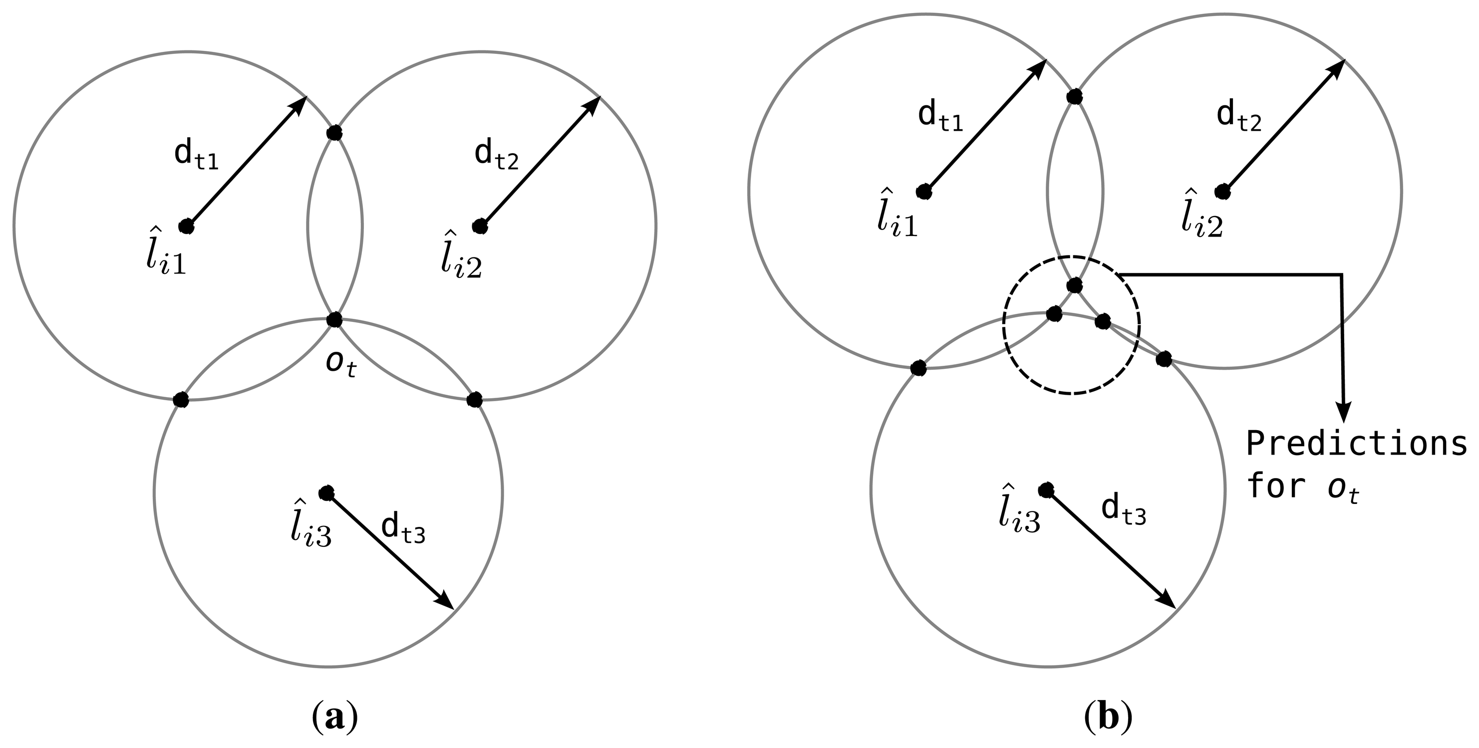
As noted earlier, only three elements in dt are sufficient for calculating the location of the reference point via trilateration [29]. Hence, let us first consider the case of having three location estimates in L̂i, say l̂i1, l̂i2 and l̂i3. SeLL forms three circles (Ci1, Ci2 and Ci3) and finds two points of intersection for each of two-circle combinations of three circles, resulting in six intersection points (Figure 3). Among them, three points, one from each two-circle pair, that are closer to one another are selected. Then the reference point is within the triangle defined by these three points. With perfect inputs these three points overlap and the location of the reference point can be calculated with point accuracy, whereas the surface area of the estimation triangle increases as the error increases. Next, when the size of L̂i is greater than 3, the redundancy in dt can be used to enhance the quality of L̂i. That is, the location of the target is calculated with all combinations of two-circle pairs, {(Cik, Cim) | k ≠ m} and corresponding distance measurements, {(dtk, dtm) | k ≠ m} by using the intersection of two circles.
The location of the reference point, although unknown, is the same across dt, and hence, we define a prediction error at time t, denoted by eit, as the aggregate difference between calculated locations of the reference point from the circle pairs. The Distance of L̂i is then given by the sum of all eit’s over the rows of
. In Figure 3, ot denotes the actual location of the target at time t. As illustrated in Figure3a, eit = 0 if L̂i is the global minimum solution and there is no error in the distance measurements. However, the predictions for ot do not overlap for an inferior L̂i and eit > 0 as shown in Figure3b. The pseudo code for a simplified Distance function is given in Algorithm 2.
| Algorithm 2: Simplified Distance function |
| Function Distance(L̂i,
) begin |
| Distance = 0; |
| foreach dt ∈ D do |
| O′ = {}; |
| foreach l̂ik ∈ L̂i and l̂im ∈ L̂i, k ≠ m do |
| Cik = circle with radius dtk centered at l̂ik; |
| Cim = circle with radius dtm centered at l̂im; |
| o1, o2 = IntersectionPoints(L̂i,Cik, Cim); |
| Add o1, o2 to O′; |
| end |
| O = points from O′ that are closest to each other; |
| eit = Σ pairwiseDistances(O); |
| Distance = Distance + eit; |
| end |
| end |
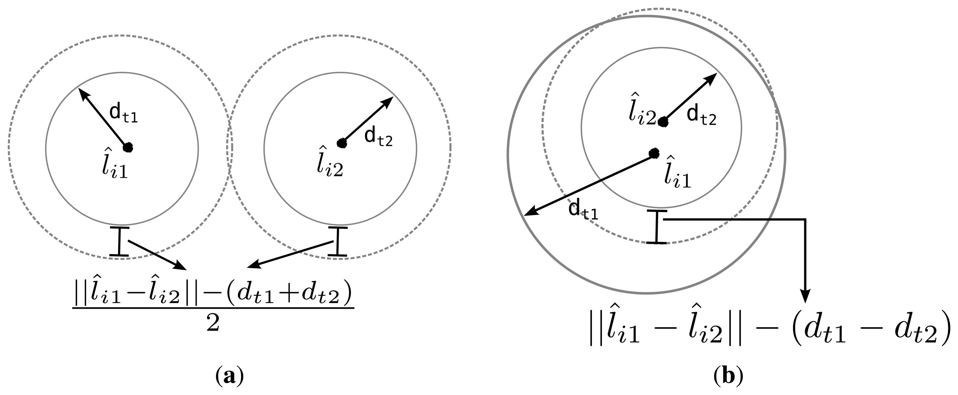
We further develop an algorithm for calculating the intersection points to deal with the cases in which some circle pairs do not overlap. We are concerned with the quality of L̂i, i.e., it’s ability to solve dt, rather than the actual measurement error, the main source of which is the prediction error. To calculate the intersection points of two circles Cik and Cim, we first compute a Euclidean distance between the centers of the circles as . Depending on the Euclidean distance, three exceptional cases may arise: (1) if ∥l̂ik − l̂im∥ > dtk + dtm then Cik and Cim are separate and there is no intersection; (2) if ∥l̂ik − l̂im∥ < |dtk + dtm|, then one circle is contained within the other and there is no intersection; and finally, (3) if ∥l̂ik − l̂im∥ = 0, dtk = dtm then the two circles coincide and there are infinite number of intersections. Note that, even though two candidate estimations L̂i and L̂j may both fall into the first case and yield no intersection, it is desirable that the Distance function assigns a lower rank for the candidate which is closer to the real topology L. Notably, simply assigning a constant large penalty to infeasible estimates results in poor performance and significantly increases the search time. Therefore, when two circles do not intersect due to case 1, we enlarge both of the circles by an equal amount so that they intersect. Likewise, if one is contained in the other, the inner circle is extended. These two cases are illustrated in Figure 4 a,b, respectively. When either case is encountered, the individual is penalized by the amount proportional to the total expansion of both circles. This process is summarized in Algorithm 3.
| Algorithm 3: A function for calculating the intersection points |
| Function IntersectionPoints (L̂i,Cik, Cim) begin |
| if Cik ∩ Cim ≠ Ø then |
| return Cik ∩ Cim; |
| end |
| else if ∥l̂ik − l̂im∥> dtk + dtm then |
| // Cik and Cim are separate |
| Δe =∥l̂ik − l̂im∥ − (dtk + dtm); |
| punish L̂i by Δe; |
| return (Cik + Δe/2) ∩ (Cim + Δe/2); |
| end |
| else if ∥l̂ik − l̂im∥ < |dtk − dtm| then |
| // Once circle is inside the other |
| Δe = |dtk − dtm| − ∥l̂ik − l̂im∥; |
| punish L̂i by Δe; |
| if dik < dim then |
| return (Cik +Δe) ∩ Cim; |
| else |
| return (Cim +Δe) ∩ Cik; |
| end |
| end |
| end |
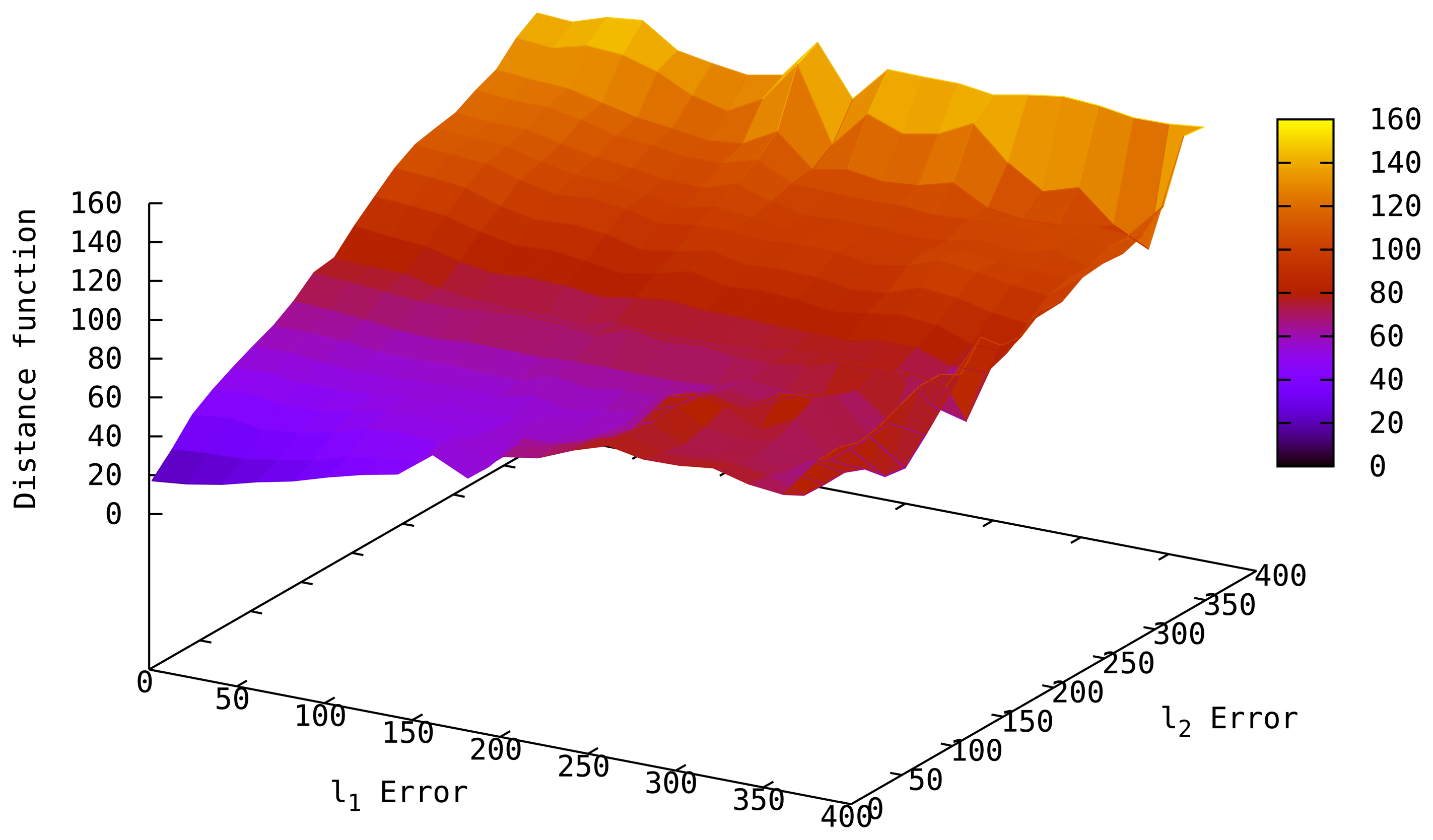
Figure 5 shows the behavior of the Distance function with varying localization error in two sensors of a 4-sensor network when the remaining two sensors have perfect predictions. We observe the Distance function can correctly assess the quality of L̂i, such that, as the estimations deviate from the actual locations, the Distance of L̂i increases. This behavior also allows us to detect sensor displacements after localization by tracking abrupt changes in the Distance of the current topology (see Section 5 for details of displacement handling). Note that the distance of L̂i may not be 0 even if L̂i = L due to measurement errors; however, it will be smaller than most of the candidates.
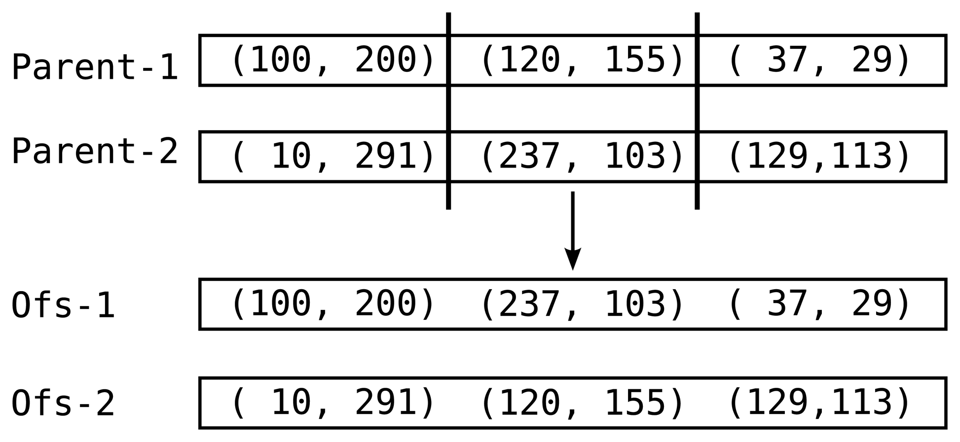
Step 2. Crossover: After the quality estimation, current population, G is sorted according to the Distance values of individuals. In addition, a new generation, G′ is created and initialized as an empty set. Pairs of individuals are then selected from G according to ranking selection that biases towards better individuals [30]. Each pair, with a probability of Rx, goes through the crossover operator. This operator randomly selects the location estimation for one sensor from one of the parents to create two offsprings (Figure 6). These offsprings are then added to the next generation G′. With a probability of 1 − Rx, input pairs are added to G′ without any changes. This crossover operation aims to collect good genes, in the sense of improving per-sensor estimations, for the individuals to help convergence to the best solution around the discovered areas of the search space [31]. The selection and pairing process continues as long as |G′| < z.
Step 3. Mutation: Each individual in G′ is modified with a probability of Rm by selecting a sensor and a coordinate axis randomly and replacing the selected value with a random value. Mutation operation prevents the search from getting stuck in a local optima by introducing new areas of exploration. The mutation rate, Rm, is generally chosen to be very small to reduce randomness. With high mutation rates, the search becomes essentially random [31,32]. Note that, we also use elitism, i.e., always keep copies of the top-ranked 3 individuals with no modification. Elitism ensures that high quality individuals survive and contribute to the next generations. Following the mutation operation, the new generation G′ becomes the new current generation G and the algorithm repeats itself for Maxgen generations [33].
5. Target Tracking and Displacement Handling
Having identified the positions of landmarks, we develop an algorithm, called Self-configuring Target Tracking (SeT), which keeps track of the location of a mobile target using distance measurements from landmarks to the target as well as monitor if some of the landmarks are displaced. The former is achieved by using trilateration to locate the target, while the latter is handled in the same way as SeLL.
In order to improve the accuracy and the robustness of tracking and to effectively handle noise-prone ultrasonic sensors, the redundancy in the number of landmarks is exploited. In particular, SeT uses K (>3) landmark sensors such that the target location is determined as the average of trilateration results of three-landmark combinations of the K landmarks as shown in Equation (1).
Although SeT can simultaneously detect and report positions of multiple targets, it cannot track the identity of multiple humans in a robust manner. For example, when two residents stop in close proximity of each other, SeT cannot maintain identities, meaning that other identification mechanisms are necessary to achieve multi-target tracking. Hence, we primarily focus on tracking a single target and reserve the latter as a future work.
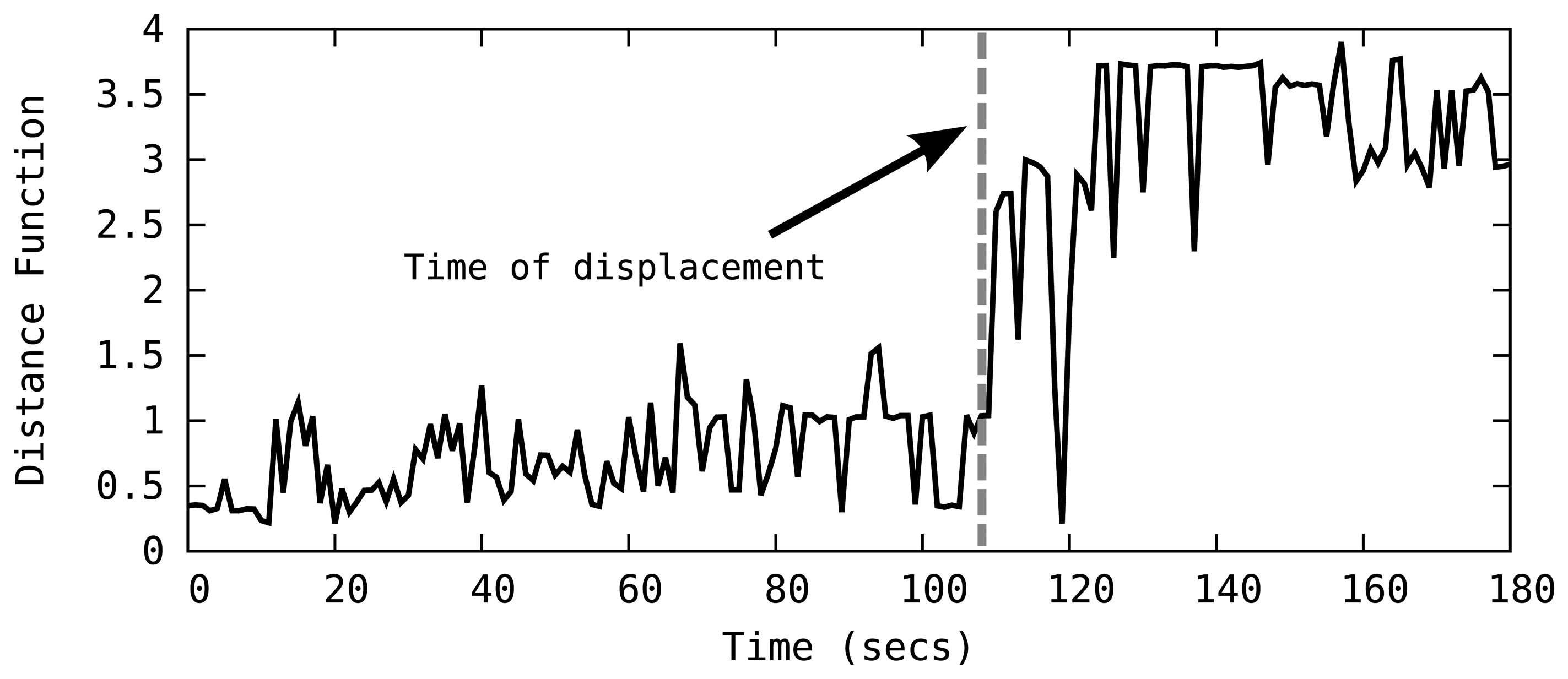
To detect landmark displacements, SeT keeps track of the Distance function as part of the tracking process, looking for fluctuations in its value, as a sudden increase in the Distance suggests a displacement of landmarks. For instance, Figure 7 plots the Distance function over time in a four-node topology, indicating one of the landmarks in the network is displaced at time t = 108. Clearly, the occurrence of displacement event is immediately reflected on the Distance function as it suddenly starts producing large values. When the system detects a displacement event, it starts a recovery phase that detects the faulty landmark and attempts to reconstruct the network topology.
We take advantage of the redundant number of landmarks, e.g., K = 4, to identify which of the landmarks has been displaced. For this purpose, we define a Distance3 function that computes the distance between the point estimations for the target locations using 3 columns in the
matrix. The Distance3 function is essentially the Distance function working only on 3 landmarks, and hence, equivalent to calculating the diameter of the prediction triangle for trilateration.
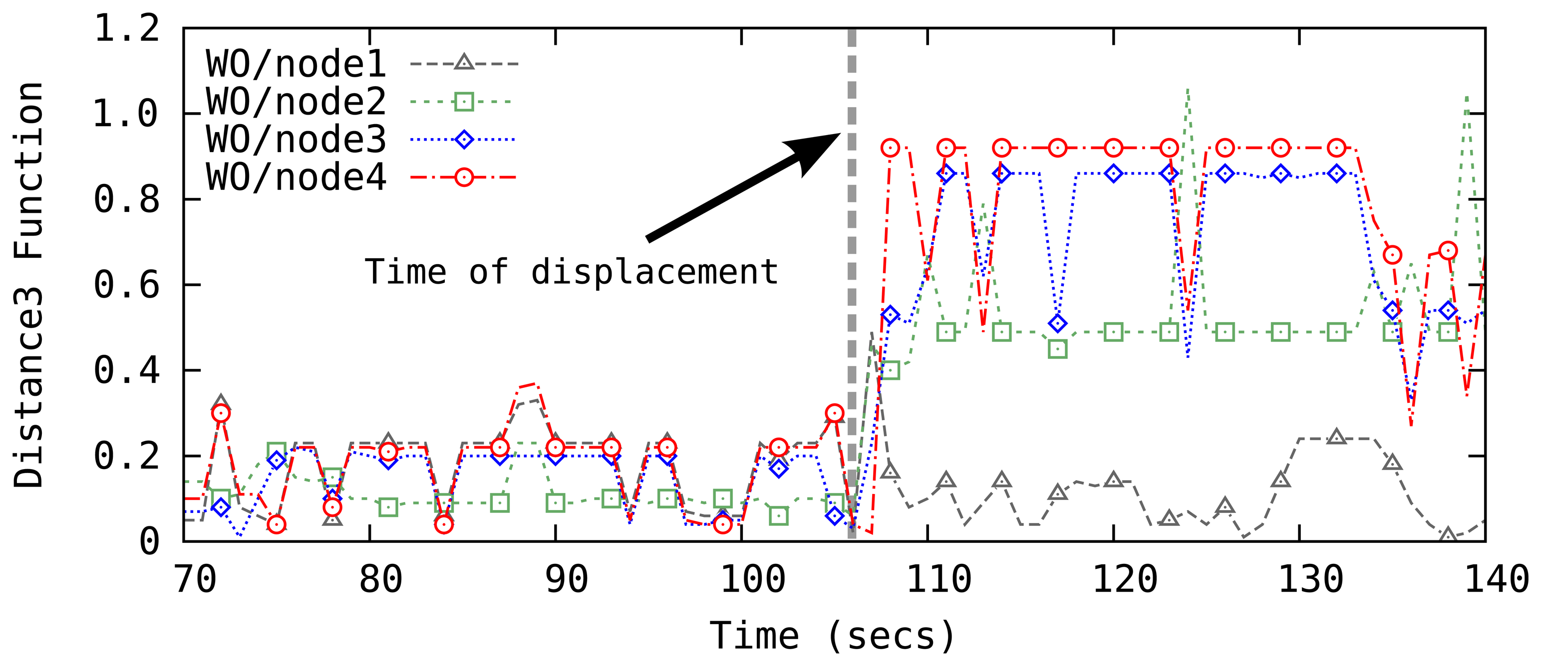
We only consider a single landmark displacement assuming that it is unlikely that multiple landmarks are relocated within a short time window. When a displacement event is detected, the system with 4 landmarks forms four sets of 3 landmarks by removing one landmark from the input and calculates the Distance3 for each of the landmark set. If one of the landmark sets yields a significantly lower Distance3 value, the landmark left out for the calculation is determined to be the displaced one and a quick recovery process is initiated. Figure 8 illustrates a case in which node1 is displaced at time t = 108. In this figure, the change in the Distance3 functions for the three-landmark sets that include node1, i.e., WO/node2–4, show a clear increase in the estimation error. In the recovery phase, a brute-force search for the current location of the displaced node is carried out. Due to low sensing range of ultrasonic ping sensors, this search is fast while the results are very accurate.
Tracking multiple objects requires modification to the SeT algorithm. First of all, an additional parameter, called an expected diameter, can be used in order to trigger the new multiple-object predictor. The algorithm can then check the diameter of a single object against the threshold and try to fit the data to a multi-object model in case exceeding the threshold. Unknowns of such a model are the number of objects, N and locations of the objects in the room, Pi, 1 ≤ i ≤ N. These unknowns can be solved through a GA formulation where an individual is encoded as a tuple (N, Pi) and the fitness being the distance between expected sensor data due to an individual and the actual sensor data. Note that stochastic minimization algorithms are observed to perform better with ultrasonic sensors due to various and frequent sources of errors.
6. Evaluation
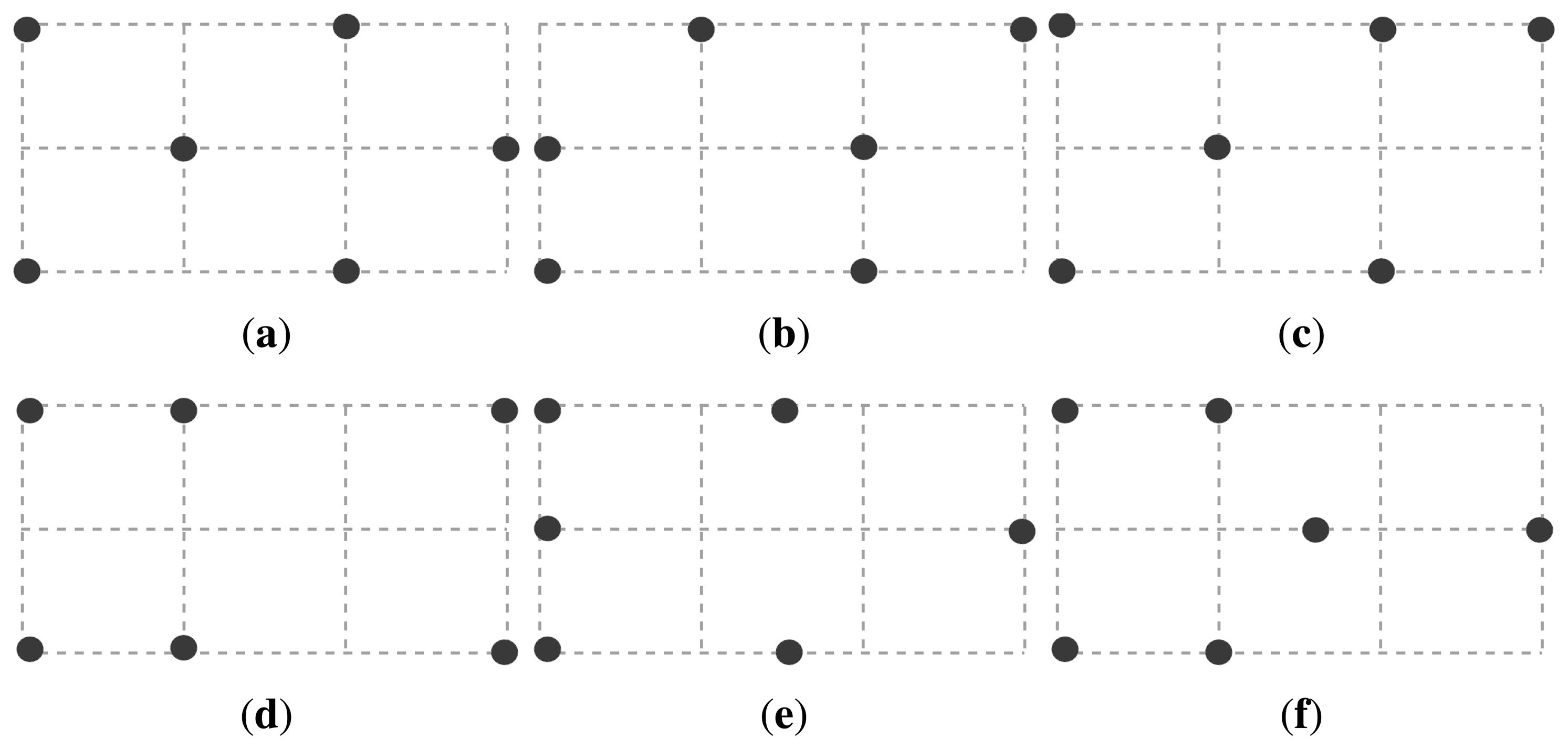
We evaluated our GA-based self-configuring localization protocol on a six-node testbed deployed within a 6 m2 room. As shown in Figure 9, a total of six different topologies were tested. We marked certain points on the ground as checkpoints. These checkpoints correspond to the intersection points of the dotted lines in Figure 9, in which, each dotted square measures 1 × 1m2. Sensor nodes are placed on these checkpoints and on the ground for ease of reconstructing the experiments, but we observe that slight differences in height from the ground do not have a significant impact on the performance of the algorithm. Sensors measure their distances to the object in a round robin fashion and wait for 0.5 s before each measurement. A participant walks between the checkpoints with no predetermined path while we record the time and the checkpoint location when the participant arrives at a checkpoint. Hence, we have the ground truth for the path taken by the participant. At some point in the experiment, we move one sensor node to an arbitrary, non-occupied checkpoint to mimic node displacement. A summary of the experimental setup and parameters for the GA are given in Table 1.
The experimental results are summarized in Table 2. To evaluate the performance of the proposed algorithm, we compute the accuracy of determining the locations of landmarks, quantified by a localization error, εL, according to Equation (2), in which L refers to the actual locations of landmarks, and lk and l̂k are the actual and estimated location of a landmark, respectively.
Equation (2) computes the total of distances between actual and estimated locations of all of the landmarks in the topology. We also calculate the maximum tracking error, εTMAX and the average tracking error, εTAVG . εTMAX is the maximum distance encountered between the actual and estimated locations of the mobile object throughout the experiments, and εTAVG is the average of these errors reported with the 90 percentile range. Moreover, we report the time the system needs to infer a node displacement as the displacement detection latency, tD. In our experiments, we only tested a single node displacement and we claim this is a common case since it is unlikely that multiple nodes are displaced as noted earlier. We also report the time, tR for recovering from a displacement. We executed our algorithm on the collected data offline so that we were able to run the algorithm multiple times on the same data, however, the system is designed to run in real-time. We report the average of 10 runs for each dataset.
As summarized in Table 2, we observe, on average, 10 cm landmark localization error. εL is relatively smaller for topologies that cover the circumference of the observed environment (Topology-1,4,5) with less than 10 cm average error for these topologies. Independent of the topology, the time to discover the locations of the landmarks during the self-configuration phase is about 6 min. This is expected since the execution flow is not heavily dependent on topological structure. Slight changes in the self configuration time are due to number of infeasible solutions generated during execution, which results in additional computations.
Maximum tracking error, εTMAX varies across topologies and it also depends on the path followed by the participant. Since we did not have a fixed path before the experiment, we cannot reliably evaluate the effect of topological formations on the tracking error. Generally, a higher landmark localization error yields higher tracking errors, and maximum observed tracking error is between 16 to 30 cm. In Table 2, we also report the average tracking error including 90 percentile error ranges. On the average, we can track a mobile target with 20 cm accuracy in a 6 m2 room.
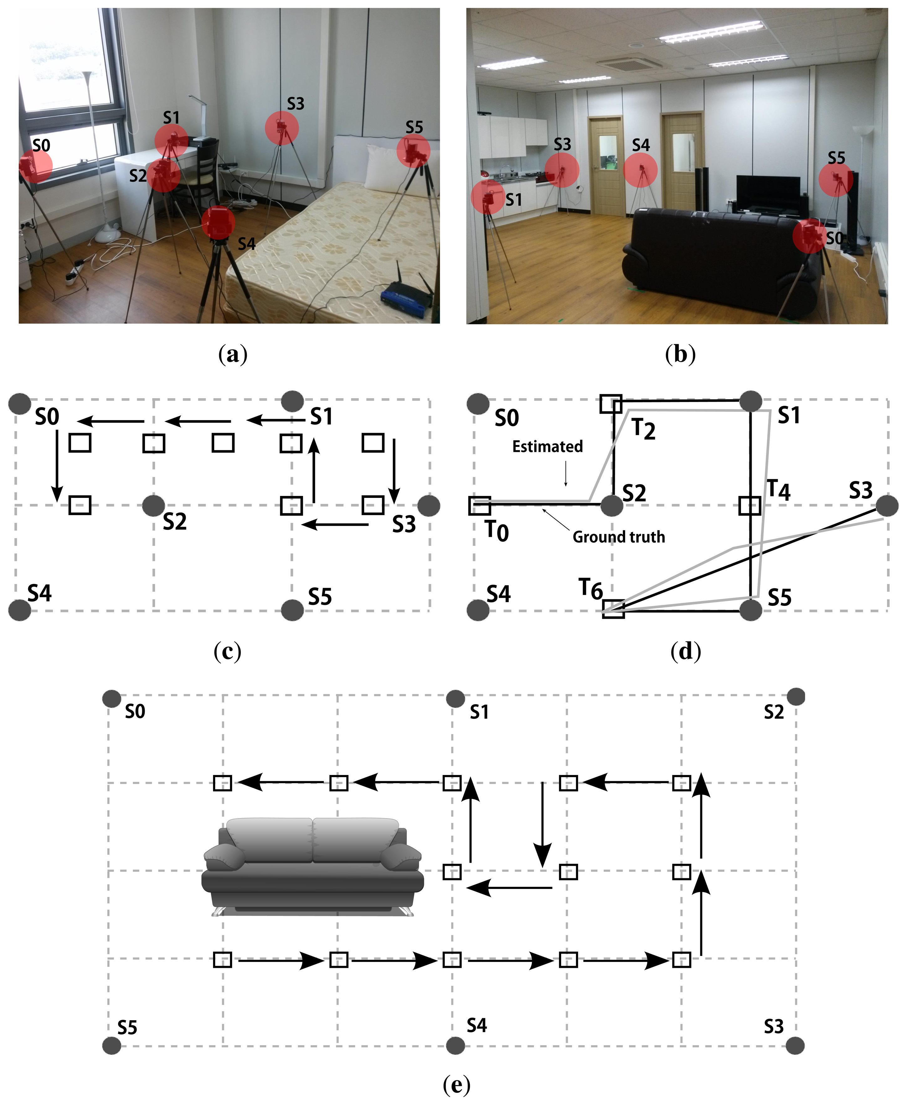
We further evaluated the tracking performance of our protocol under two topologies of different sizes, i.e., 2 × 3 m2 and 4 × 6 m2, as shown in Figure 10. We first measured the tracking performance for the testbed in Figure10c. We report 90% confidence level for 10 runs. The localization error, εL is 7.16 cm while the self-configuration time, tSC is 4.03 min. The 90 percentile maximum tracking error, εTMAX is 21.27 cm and the average tracking error, εTAVG is 11.71 cm. We also conducted a tracking test in the same testbed, and present an example tracking estimation along with the ground truth in Figure10d. Note that the black path is an approximation of the ground truth while the gray path is an estimation by the system.
We then measured the tracking performance for a larger testbed shown in Figure 10e, which is a sitting room setup with a sofa in the middle. We ran 10 experiments to report the following results. εL and tSC are 17.53 cm and 8.23 min, respectively. εTMAX is 24.46 cm while an absolute maximum tracking error over all 10 runs is 36.28 cm. Finally, εTAVG is 18.43 cm. We believe these results are satisfactory, although there is also a large room for improvement since we are putting no efforts in post processing, e.g., smoothing, the tracks generated by our system.
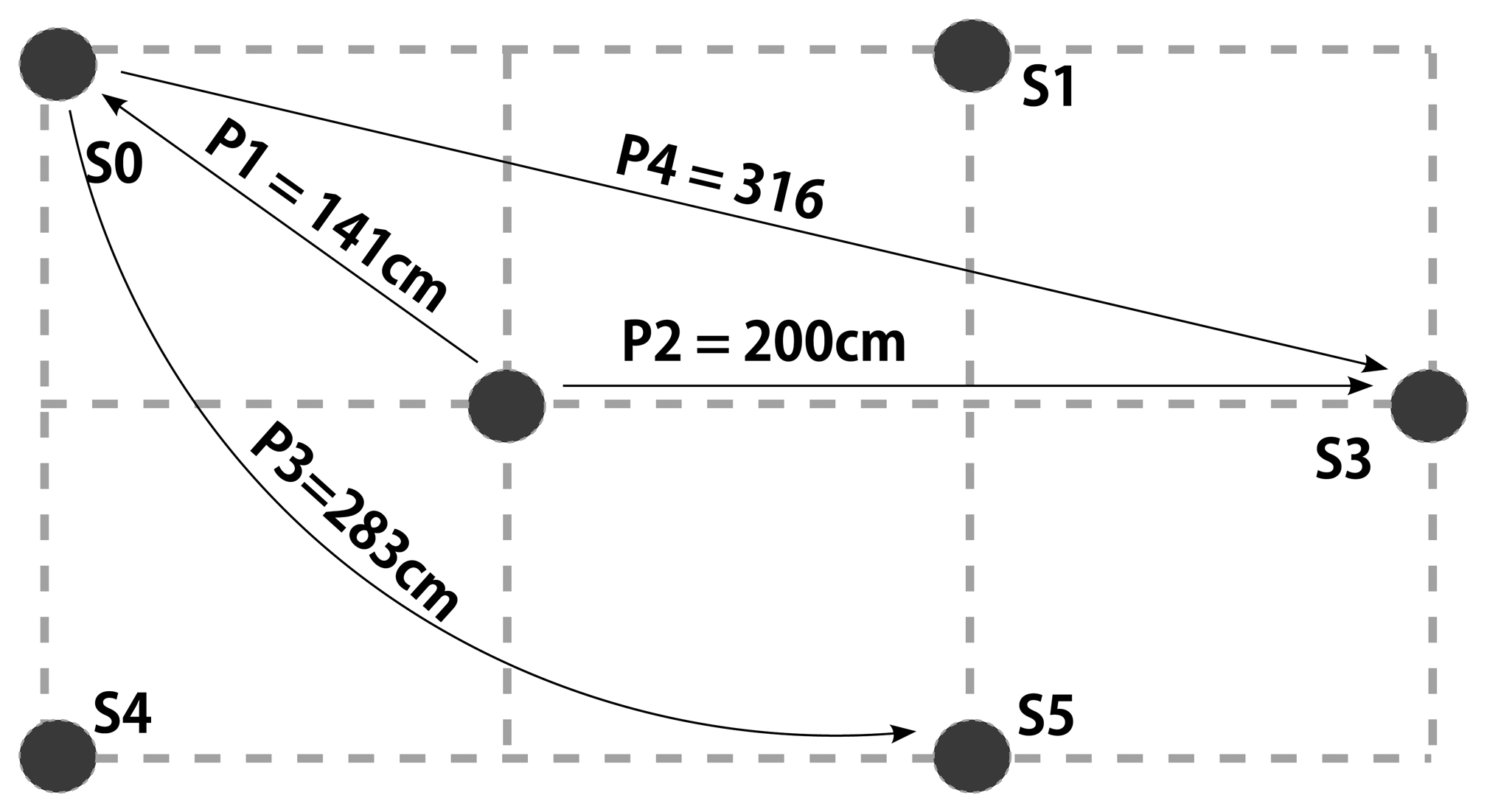
We finally evaluated the performance of our displacement detection and topology correction algorithm according to the pattern given in Figure 11. The experiments are carried out by first recording sensor data from all sensors in Figure 11, and later selectively suppressing the sensor at the target location until a predetermined time of displacement. We then suppress the source node and start streaming the target node creating a virtual displacement. This method allows us the speedup the process of analysis.
The results of the experiments are summarized in Table 3. We observe that εTMAX is inclined to increase with increasing displacement. This result is expected due to larger errors during the reconfiguration phase. Surprisingly, the magnitude of displacement does not seem to affect the detection latency. Hence, as long as there is a significant discrepancy between estimated layout and sensor data, the system can infer a displacement. The latency of detection is approximately 30 s and we do not expect to see lower values with our hardware because the system should be carefully designed in order not to enter into the reconfiguration phase frequently. Note that even multi-path effects may cause such discrepancies. Nevertheless, this latency can still be further reduced using higher quality sensors. Similarly, the recovery time, tR, after a displacement does not seem to depend on the magnitude of the displacement. Rather, we consider that the time required for reconfiguration is a function of the resulting topology. We observe that within 5 s of the detection, the system reconstructs the model.
7. Conclusions and Future Work
In this paper, we presented a self-configuration protocol for device-free target tracking systems. The proposed protocol first maps the geographic topology of a network of low-cost ultrasound sensors without using nodes with known locations, then proceeds to track humans using the same hardware. We also developed a lightweight sensor displacement scheme that can detect any changes in the topology in less than a minute and initiate a quick recovery phase to generate a new map within seconds. Finally, we demonstrated via experiments that our proposed system can produce highly accurate results over a broad range of network layouts. In the future, we will extend our tracking system to add the capability of tracking multiple targets.
Acknowledgments
This research was supported in part by the DGIST R&D Program of MSIP of Korea (CPS Global Center), and in part by the IT R&D Program of MSIP/IITP (10041145, Self-Organized Software platform for Welfare Devices).
Author Contributions
Can Basaran proposed the main ideas, designed the protocol, performed experiments, and wrote the paper. Jong-Wan Yoon performed experiments, and gave helpful comments to edit the paper. Sang H. Son discussed the key ideas and gave helpful comments to edit the paper. Taejoon Park suggested and discussed the key ideas, led the project, and edited the paper. All authors contributed to the paper.
Conflicts of Interest
The authors declare no conflict of interest.
References
- Lu, C.H.; Wu, C.L.; Fu, L.C. A Reciprocal and Extensible Architecture for Multiple-Target Tracking in a Smart Home. Syst. Man Cybern. C 2011, 41, 120–129. [Google Scholar]
- Hnat, T.W.; Griffiths, E.; Dawson, R.; Whitehouse, K. Doorjamb: Unobtrusive Room-Level Tracking of People in Homes Using Doorway Sensors. Proceedings of the 10th ACM Conference on Embedded Network Sensor Systems, Toronto, ON, Canada, 6–9 November 2012; ACM: New York, NY, USA, 2012; pp. 309–322. [Google Scholar]
- Jain, S.; Sabharwal, A.; Chandra, S. An Improvised Localization Scheme using Active RFID for Accurate Tracking in Smart Homes. Proceedings of the 2010 12th International Conference on Computer Modelling and Simulation (UKSim), Cambridge, UK, 24–26 March 2010; pp. 51–56.
- Han, G.; Xu, H.; Duong, T.Q.; Jiang, J.; Hara, T. Localization Algorithms of Wireless Sensor Networks: A Survey. Telecommun. Syst. 2011, 52, 2419–2436. [Google Scholar]
- Bulusu, N.; Heidemann, J.; Estrin, D. GPS-Less Low-Cost Outdoor Localization for Very Small Devices. Pers. Commun. 2000, 7, 28–34. [Google Scholar]
- Mao, G.; Fidan, B.; Anderson, B. Wireless Sensor Network Localization Techniques. Comput. Netw. 2007, 51, 2529–2553. [Google Scholar]
- Sugihara, R.; Gupta, R.K. Sensor Localization with Deterministic Accuracy Guarantee. Proceedings of the 30th IEEE International Conference on Computer Communications, Shanghai, China, 10–15 April 2011; pp. 1772–1780.
- Kulkarni, R.V.; Forster, A.; Venayagamoorthy, G.K. Computational intelligence in wireless sensor networks: A survey. Commun. Surv. Tutor. 2011, 13, 68–96. [Google Scholar]
- Shaha, R.K.; Mahmud, N.; Bin Zafar, R.; Rahman, S. Development of Navigation system for visually impaired person. In Ph.D. Thesis; EEE Department, BRAC Unviersity: Dhaka, Bangladesh, 2012. [Google Scholar]
- Want, R.; Hopper, A. Active Badges and Personal Interactive Computing Objects. Consum. Electron. 1992, 38, 10–20. [Google Scholar]
- Priyantha, N.B.; Chakraborty, A.; Balakrishnan, H. The Cricket Location-Support System. Proceedings of the Mobile Computing and Networking, Boston, MA, USA, 6–11 August 2000; ACM: New York, NY, USA, 2000; pp. 32–43. [Google Scholar]
- Harter, A.; Hopper, A.; Steggles, P.; Ward, A.; Webster, P. The anatomy of a context-aware application. Wirel. Netw. 2002, 8, 59–68. [Google Scholar]
- Bahl, P.; Padmanabhan, V.N. RADAR: An In-Building RF-based User Location and Tracking System. Proceedings of the IEEE International Conference on Computer Communications, Tel Aviv, Israel, 26–30 March 2000; Volume 2, pp. 775–784.
- Chintalapudi, K.; Padmanabha Iyer, A.; Padmanabhan, V.N. Indoor Localization without the Pain. Proceedings of the Mobile Computing and Networking, Chicago, IL, USA, 20–24 September 2010; ACM: New York, NY, USA, 2010; pp. 173–184. [Google Scholar]
- Teixeira, T.; Savvides, A. Lightweight People Counting and Localizing in Indoor Spaces Using Camera Sensor Nodes. Proceedings of the IEEE Distributed Smart Cameras, Vienna, Austria, 25–28 September 2007; ACM: New York, NY, USA, 2007; pp. 36–43. [Google Scholar]
- Xu, C.; Firner, B.; Moore, R.S.; Zhang, Y.; Trappe, W.; Howard, R.; Zhang, F.; An, N. SCPL: Indoor Device-Free Multi-Subject Counting and Localization using Radio Signal Strength. Proceedings of the Information Processing in Sensor Networks, Philadelphia, PA, USA, 8–11 April 2013; ACM: New York, NY, USA, 2013; pp. 79–90. [Google Scholar]
- Kumar, A.; Khosla, A.; Saini, J.S.; Singh, S. Computational Intelligence based Algorithm for Node Localization in Wireless Sensor Networks. Proceedings of the IEEE Intelligent Systems, Sofia, Bulgaria, 6–8 September 2012; pp. 431–438.
- Yun, S.; Lee, J.; Chung, W.; Kim, E.; Kim, S. A Soft Computing Approach to Localization in Wireless Sensor Networks. Expert Syst. Appl. 2009, 36, 7552–7561. [Google Scholar]
- Nan, G.F.; Li, M.Q.; Li, J. Estimation of Node Localization with a Real-Coded Genetic Algorithm in WSNs. Proceedings of the IEEE Machine Learning and Cybernetics, Hong Kong, China, 19–22 August 2007; Volume 2, pp. 873–878.
- Vecchio, M.; López-Valcarce, R.; Marcelloni, F. A Two-Objective Evolutionary Approach based on Topological Constraints for Node Localization in Wireless Sensor Networks. Appl. Soft Comput. 2012, 12, 1891–1901. [Google Scholar]
- Marks, M.; Niewiadomska-Szynkiewicz, E. Two-Phase Stochastic Optimization to Sensor Network Localization. Proceedings of the IEEE Sensor Technologies and Applications, Valencia, Spain, 14–20 October 2007; pp. 134–139.
- Chen, G.; Hong, L. A Genetic Algorithm Based Multi-Dimensional Data Association Algorithm for Multi-Sensor? Multi-Target Tracking. Math. Comput. Model. 1997, 26, 57–69. [Google Scholar]
- Turkmen, I.; Guney, K.; Karaboga, D. Genetic Tracker with Neural Network for Single and Multiple Target Tracking. Neurocomputing 2006, 69, 2309–2319. [Google Scholar]
- Prallax PING Utrasonic Distance Sensor, 28015. Available online: http://www.parallax.com/dl/docs/prod/acc/28015-PING-v1.3.pdf (accessed on 15 April 2014).
- Lazik, P.; Rowe, A. Inddor pseudo-ranging of mobile devices using ultrasonic chirps. Proceedings of the ACM SenSys 2012, Toronto, Canada, 6–9 November 2012; pp. 99–112.
- Liu, K.; Liu, X.; Xie, L.; Li, X. Towards accurate acoustic localization on a smartphone. Proceedings of the IEEE INFOCOM 2013, Turin, Italy, 14–19 April 2013; pp. 495–499.
- Yang, Z.; Liu, Y. Quality of Trilateration: Confidence-based Iterative Localization. Parallel Distrib. Syst. 2010, 21, 631–640. [Google Scholar]
- Ester, M.; Kriegel, H.P.; Sander, J.; Xu, X. A Density-Based Algorithm for Discovering Clusters in Large Spatial Databases with Noise. Proceedings of the Knowledge Discovery and Data Mining, Portland, OR, USA, 2–4 August 1996; Volume 96, pp. 228–231.
- Han, G.; Choi, D.; Lim, W. Reference Node Placement and Selection Algorithm Based on Trilateration for Indoor Sensor Networks. Wirel. Commun. Mobile Comput. 2009, 9, 1017–1027. [Google Scholar]
- Goldberg, D.E.; Deb, K. A Comparative Analysis of Selection Schemes Used in Genetic Algorithms. Urbana 1991, 51, 69–93. [Google Scholar]
- Chambers, L.D. Practical Handbook of Genetic Algorithms: Complex Coding Systems; CRC Press: Boca Raton, FL, USA, 2010; Volume 3. [Google Scholar]
- Ochoa, G. Error thresholds in genetic algorithms. Evol. Comput. 2006, 14, 1–19. [Google Scholar]
- Kulkarni, R.V.; Venayagamoorthy, G.K.; Cheng, M.X. Bio-Inspired Node Localization in Wireless Sensor Networks. Proceedings of the IEEE Systems, Man and Cybernetics, San Antonio, TX, USA, 11–14 October 2009; pp. 205–210.


| Parameter | Value |
|---|---|
| Number of generations | 400 |
| Population size | 100 |
| Mutation rate (Rm) | 0.1 |
| Crossover rate (Rx) | 0.6 |
| Number of elites | 3 |
| Area size | 3 × 2 (m2) |
| Number of sensors | 6 |
| Sensing delay | 0.5 (s) |
| Topology | εL (cm) | tSC (min) | εTMAX (cm) | εTAVG (cm) | tD (s) | tR (s) |
|---|---|---|---|---|---|---|
| Topology-1 | 8.23 | 5.69 | 19.62 | 12.47 ± 3.56 | 24.64 | 3.14 |
| Topology-2 | 12.87 | 5.71 | 29.50 | 16.39 ± 7.01 | 36.71 | 3.92 |
| Topology-3 | 13.60 | 5.32 | 25.21 | 14.21 ± 6.22 | 43.37 | 3.11 |
| Topology-4 | 5.41 | 5.43 | 22.09 | 9.57 ± 8.19 | 21.09 | 3.49 |
| Topology-5 | 9.21 | 4.98 | 23.42 | 12.13 ± 9.08 | 29.50 | 2.91 |
| Topology-6 | 14.40 | 6.07 | 16.01 | 6.08 ± 7.56 | 33.99 | 3.06 |
| Scenario | Distance (cm) | εTMAX (cm) | εTAVG (cm) | tD (s) | tR (s) |
|---|---|---|---|---|---|
| P1 | 141 | 17.53 | 8.50 ± 3.17 | 27.47 | 3.24 |
| P2 | 200 | 16.01 | 7.23 ± 2.52 | 30.34 | 2.19 |
| P3 | 283 | 23.38 | 11.19 ± 2.46 | 32.45 | 4.54 |
| P4 | 316 | 29.14 | 13.03 ± 2.14 | 30.32 | 3.37 |
© 2014 by the authors; licensee MDPI, Basel, Switzerland. This article is an open access article distributed under the terms and conditions of the Creative Commons Attribution license ( http://creativecommons.org/licenses/by/4.0/).
Share and Cite
Basaran, C.; Yoon, J.-W.; Son, S.H.; Park, T. Self-Configuring Indoor Localization Based on Low-Cost Ultrasonic Range Sensors. Sensors 2014, 14, 18728-18747. https://doi.org/10.3390/s141018728
Basaran C, Yoon J-W, Son SH, Park T. Self-Configuring Indoor Localization Based on Low-Cost Ultrasonic Range Sensors. Sensors. 2014; 14(10):18728-18747. https://doi.org/10.3390/s141018728
Chicago/Turabian StyleBasaran, Can, Jong-Wan Yoon, Sang Hyuk Son, and Taejoon Park. 2014. "Self-Configuring Indoor Localization Based on Low-Cost Ultrasonic Range Sensors" Sensors 14, no. 10: 18728-18747. https://doi.org/10.3390/s141018728
APA StyleBasaran, C., Yoon, J.-W., Son, S. H., & Park, T. (2014). Self-Configuring Indoor Localization Based on Low-Cost Ultrasonic Range Sensors. Sensors, 14(10), 18728-18747. https://doi.org/10.3390/s141018728