Introduction

Sensors

1424-8220

Molecular Diversity Preservation International (MDPI)

10.3390/s120912545

sensors-12-12545

Article

Sunglint Detection for Unmanned and Automated Platforms

Garaba

Shungudzemwoyo Pascal

¹^* Schulz

Jan

¹ Wernand

Marcel Robert

² Zielinski

Oliver

1. Institute for Chemistry and Biology of the Marine Environment—Terramare, Carl von Ossietzky University of Oldenburg, Schleusenstraβe 1, Wilhelmshaven 26382, Germany; E-Mails: jan.schulz@uni-oldenburg.de (J.S.); oliver.zielinski@uni-oldenburg.de (O.Z.) 2. Royal Netherlands Institute for Sea Research, Physical Oceanography, Marine Optics & Remote Sensing, P.O. Box 59, Den Burg, Texel 1790AB, The Netherlands; E-Mail: marcel.wernand@nioz.nl

* Author to whom correspondence should be addressed; E-Mail: shungu.garaba@uni-oldenburg.de; Tel.: +49-4421-778-5817; Fax: +49-4421-778-5823.

2012

13 09 2012

12 9 12545 12561 14 07 2012 20 08 2012 29 08 2012

2012

This article is an open access article distributed under the terms and conditions of the Creative Commons Attribution license (http://creativecommons.org/licenses/by/3.0/).

We present an empirical quality control protocol for above-water radiometric sampling focussing on identifying sunglint situations. Using hyperspectral radiometers, measurements were taken on an automated and unmanned seaborne platform in northwest European shelf seas. In parallel, a camera system was used to capture sea surface and sky images of the investigated points. The quality control consists of meteorological flags, to mask dusk, dawn, precipitation and low light conditions, utilizing incoming solar irradiance (E_S) spectra. Using 629 from a total of 3,121 spectral measurements that passed the test conditions of the meteorological flagging, a new sunglint flag was developed. To predict sunglint conspicuous in the simultaneously available sea surface images a sunglint image detection algorithm was developed and implemented. Applying this algorithm, two sets of data, one with (having too much or detectable white pixels or sunglint) and one without sunglint (having least visible/detectable white pixel or sunglint), were derived. To identify the most effective sunglint flagging criteria we evaluated the spectral characteristics of these two data sets using water leaving radiance (L_W) and remote sensing reflectance (R_RS). Spectral conditions satisfying ‘mean L_W (700–950 nm) < 2 mW·m⁻²·nm⁻¹·Sr⁻¹’ or alternatively ‘minimum R_RS (700–950 nm) < 0.010 Sr⁻¹’, mask most measurements affected by sunglint, providing an efficient empirical flagging of sunglint in automated quality control.

sunglint empirical quality control ocean colour coastal and shelf seas hyperspectral sensing

1. Introduction

Automated and unmanned remote sensing from above-water, airborne and satellite platforms is a non-invasive approach in observing marine biochemical and geophysical characteristics on a regional or global scale [1–3]. Inevitably remote sensing measurements from these platforms are prone to meteorological conditions and sunglint contamination. Sunglint is a transient anomaly that occurs when sunlight is reflected from the seawater surface directly into the down looking optical sensor [4,5]. It is a product of Fresnel reflection from a number of ‘dancing facets’ on a wind disturbed seawater surface. Sunglint is influenced by the position of the sun, viewing angle of the optical sensor, water refractive index, cloud cover, wind direction, and speed [6–8].

Kay et al. [9] assessed sunglint correction models for optical measurements in marine environments identifying that most of the models rely partly on the black pixel assumption [10] and tend to some extent correct glint pixels. The black pixel assumption postulates that water leaving radiance is insignificant in the near infra-red spectrum. However, several reports have shown that in coastal and turbid waters this assumption is not valid. Hence correction models employing this assumption have a high probability of over- or underestimation of apparent and inherent optical properties [5,10–12]. Thus, development of a further sunglint flag for masking obviously contaminated measurements is desirable, hence minimising the probability of errors likely to occur when using correction models.

Wernand [13] described a meteorological quality flagging method to optimise automated hyperspectral measurements for coastal and shelf seas. It masks incoming solar irradiance (E_S) taken during low light, dusk, dawn and under rainfall. Additionally, to reduce measurements affected by sunglint he suggests the use of two optical sensors looking in different azimuthal directions to measure water surface leaving radiance. The lowest water surface leaving radiance for each measurement is then assumed to have the least sunglint. While this setup is useful and minimises sunglint effects on measurements, it requires additional sensors to be installed and there is a possible risk of sunglint affecting both sensors.

In this report we aim to derive sunglint quality control flags for automated and unmanned above-water hyperspectral measurements to complement meteorological flags reported by Wernand [13]. For validation we use sky and sea surface images from a simultaneously operated camera system. The automatic sunglint detection algorithm is implemented to provide an objective way of distinguishing sunglint from non-sunglint situations.

2. Data and Methods

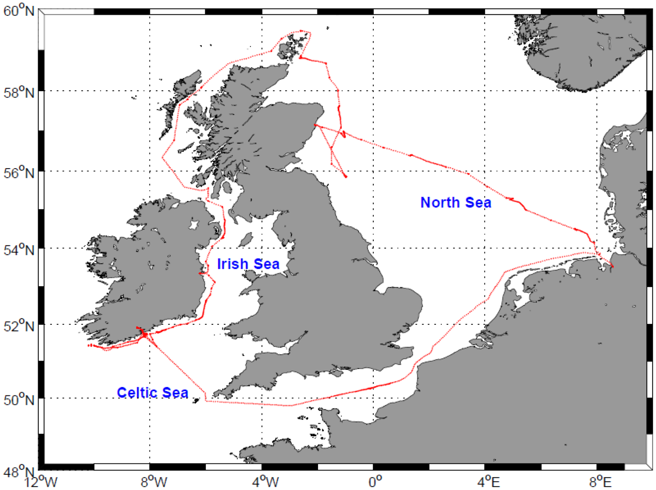
Above-water hyperspectral radiometric measurements were conducted aboard the R/V Heincke cruise HE302, between 21 April and 14 May 2009 in the northwest European shelf seas (Figure 1). The campaign was within the scope of the North Sea Coast Harmful Algal Bloom (NORCOHAB II) field campaign.

2.1. Instrumentation

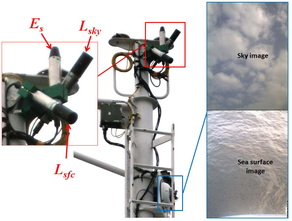
A RAMSES-ACC hyperspectral cosine irradiance meter (TriOS, Germany) was used to measure incoming solar radiation, E_S (λ). Two RAMSES-ARC hyperspectral radiance meters (7° field-of-view in air), were used to detect the sea surface radiance L_sfc (θ_sfc, Φ, λ) and sky radiance L_sky (θ_sky, Φ, λ). A frame (see Figure 2) designed to hold the irradiance sensor facing upwards, with the sky and sea surface radiance sensors at zenith angles θ_sfc = 45° and θ_sky = 135°, was fixed to the mast of the ship facing starboard, 12 m above sea surface. These spectral measurements were automatically collected at 15 min intervals over a spectral range λ = 320–950 nm in steps of 5 nm.

A DualDome D12 (Mobotix AG, Langmeil, Germany) camera system with field-of-view set to 45°, was used to capture sky and sea surface images simultaneous to hyperspectral measurements, as illustrated in Figure 2. Positioning height (∼12 m above sea surface) of camera and optical sensors proved to be unaffected by sea spray. The camera's field-of-view was set congruent with the area observed by the radiometers, L_sky and L_sfc. Ship's position and heading were recorded by a Differential Global Position System (DGPS) and sampling times were logged in Coordinated Universal Time (UTC).

2.2. Methods

The first quality control step involved implementing the meteorological flagging [13] on E_S (λ) measurements using MATLAB 2010a (The MathWorks, GmbH, Ismaning, Germany). The three meteorological flag conditions are:

E_S (λ = 480 nm) > 20 mW·m⁻²·nm⁻¹ setting a threshold for which significant E_S (λ) can be measured,

E_S (λ = 470 nm)/E_S (λ = 680 nm) < 1 masking spectra affected by dawn/dusk radiation,

E_S (λ = 940 nm)/E_S (λ = 370 nm) < 0.25 masking spectra affected by rainfall and high humidity.

E_S (λ) that passed this meteorological flagging and corresponding L_sfc (θ_sfc, Φ, λ), L_sky (θ_sky, Φ, λ) measurements were used to derive water leaving radiance, L_W (θ_sfc, Φ, λ), and remote sensing reflectance, R_RS (θ, Φ, λ) according to Equation (1) [14]: (1) R R S = L W E S = L sfc − ( ρ air − sea ⋅ L sky ) E Swhere ρ_air-sea is the air-sea interface reflectance factor assumed to be ρ_air-sea = 0.0256 correcting for sky reflected radiation. We tested the performance of sunglint correction models by Gould et al. [5] Mobley [8], Lee et al. [4] and Ruddick et al. [15] using its cloud cover and wind components of Ruddick et al. [15] (see Supplementary Material). Optical measurements and computed parameters can be freely accessed via the PANGAEA database of the World Data Center for Marine Environmental Sciences (WDC-Mare, http://www.pangaea.de): http://www.doi.pangaea.de/10.1594/PANGAEA.759690.

2.2.1. Automated Sunglint Image Detection Algorithm

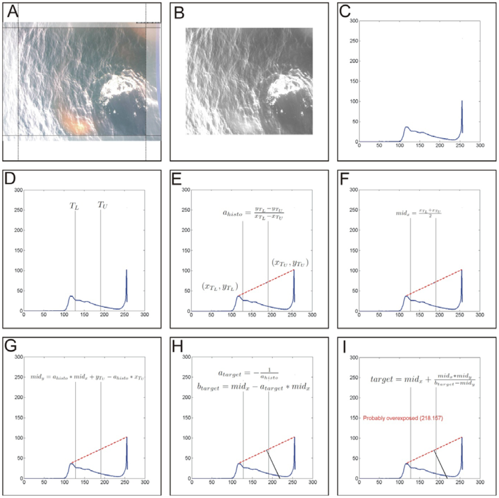
A well exposed digital greyscale image of the sea surface normally shows several peaks scattered across the grey level histogram. Between peaks the histogram shows plateaus and has an averaged centred and balanced density distribution. When overexposed, images show a significant higher count of bright colours with white dominating. Consequently, the density distribution in the histogram shifts characteristically towards the white end where mostly one prominent peak is observed. The proposed automated sunglint detection algorithm is based on simple histogram arithmetic to evaluate the gray value ratio between dominating dark and bright counts (see Figure 3).

Processing of each full colour (24 bit colour depth) image starts with cropping image borders for 5% on all sides. As the camera is mounted stationary on the mast, field of view is prone to ship movements. Cropping has the advantage to reduce wash and white caps close to the vessel's hull, the hull itself or atmospheric interferences, depending on displacement from the vertical. Additionally it focuses the evaluated part of the image to the reading spot of the hyperspectral radiometer on the sea surface.

The cropped colour image is converted to greyscale and colour depth is reduced to b bits (with b < 24). In our case we use b = 8, resulting in a normal greyscale image with 256 levels. The histogram is computed for the greyscale image, normalised and multiplied by 2^b.

Prior to determining the bright/dark ratio a lower (T_L) and upper (T_U) threshold is defined, with constraints 0 ≤ T_L < T_U < 2^b. Threshold used here have been identified empirically and are in good congruence with results obtained by a human investigator. A value T_L = 2^b/2 is a suitable first, and T_U = 2^b × 0.75 second threshold (respectively values 128 and 192 for a 2⁸ level greyscale image). In the histogram local maxima are identified within the intervals 0 ≤ × ≤ T_L and T_U ≤ × < 2^b. Values between T_L < × < T_U are excluded.

Between the two maxima a line segment is created and its slope calculated. The perpendicular to the line segment is calculated, intersecting it at the half of the length of the line segment. A special case appears if the slope of the line segment is zero, as it results in a division by zero when calculating the slope of the perpendicular. In this case a vertical line is created instead. With the previously defined constraints the slope cannot become infinity.

The intersection of the finally determined straight line with the abscissa is used as indicator for overexposure. If this value is larger than T_U the image is tagged as potentially overexposed.

2.2.2. Spectral Analysis for Sunglint Flag

The empirical sunglint flag, based on spectral information, was developed on the premise that open seawater is assumed to absorb all light in the NIR. Thus, any light signal measured by an optical sensor would be sea surface reflectance or atmospheric scattered radiance. However, in turbid waters multiple scattering influenced by optically active seawater constituents also contributes to this light signal measurable by an optical sensor [5,12,16]. Removing a fraction ρ_air-sea of the sky radiance L_sky has become standard procedure to minimise sunglint in water leaving radiance L_W from, above-water remote sensing. However, this approach like any correction model does not fully guarantee sunglint free measurements [4,8].

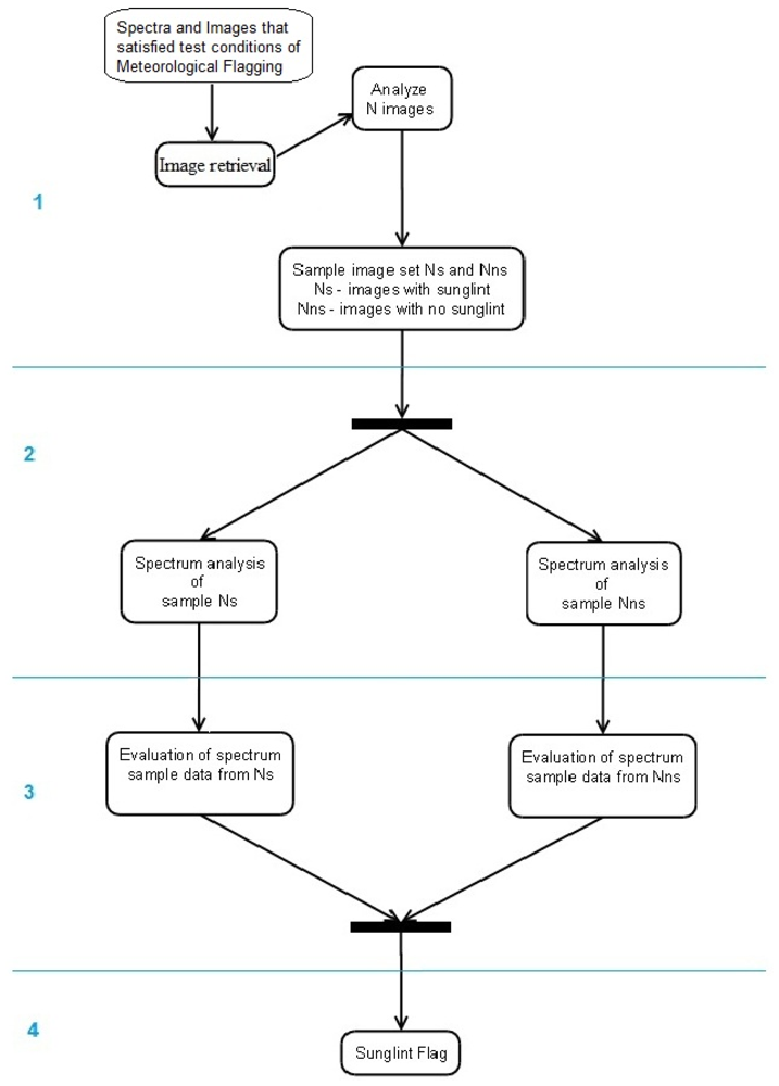
Our objective is to provide a reliable sunglint flagging with the advantage of sea-surface images to validate an empirical spectral approach to eliminating measurements affected by sunglint. In Figure 4 a simplified activity diagram illustrates the steps that were implemented in this sunglint flag investigation and evaluation:

The automated sunglint image detection algorithm (Section 2.2.1) was applied to sea surface images that are matching the unmasked spectra validated with the meteorological flagging [13]. Based on the computed probability of sunglint contamination in the images, they were classified into Nns–image set without sunglint or Ns–sunglint-affected image set.

Spectra analysis of the two sets Nns and Ns was used to identify unique characteristics with respect to L_W (λ) and R_RS (λ). This included the investigation of each individual spectra and mean spectra for the two sets over the whole spectrum range (λ = 320–950 nm), to obtain a general overview on typical spectra for the sets Nns and Ns;

To obtain distinguishing features for spectra data sets in Ns and Nns utilising findings from step 2 (i.e., spectrum shape, behaviour and magnitude variations of both L_W (λ) and R_RS (λ) in the VIS and NIR) a combination of inequality equations and band ratios was implemented. These combinations include:

using the NIR mean spectra to obtain threshold values unique in set Nns and Ns. This procedure was repeated using the NIR minimum spectra obtained from the statistical analysis of the Nns and Ns sets respectively,

performing spectral band ratioing on characteristic spectral bands both in VIS and NIR, here λ = 400 nm, 460 nm, 760 nm, 940 nm [9,13,17].

To test the performance of the above mentioned procedures a reanalysis of the original united data set of all valid spectra from step 1 was run. Based on the comparison of this computation with the independent image algorithm (Section 2.2.1.) effective sunglint flagging criteria were identified.

3. Results and Discussion

A total of 629 from 3,121 spectral measurements passed the test conditions of the meteorological flagging. The image assessment of these unmasked 629 spectra came up with 501 images free of sunglint, Nns (having least visible/detectable white pixel or sunglint), and 128 sunglint-affected images, Ns (having too much or detectable white pixels or sunglint).

3.1. Sunglint Image Analysis

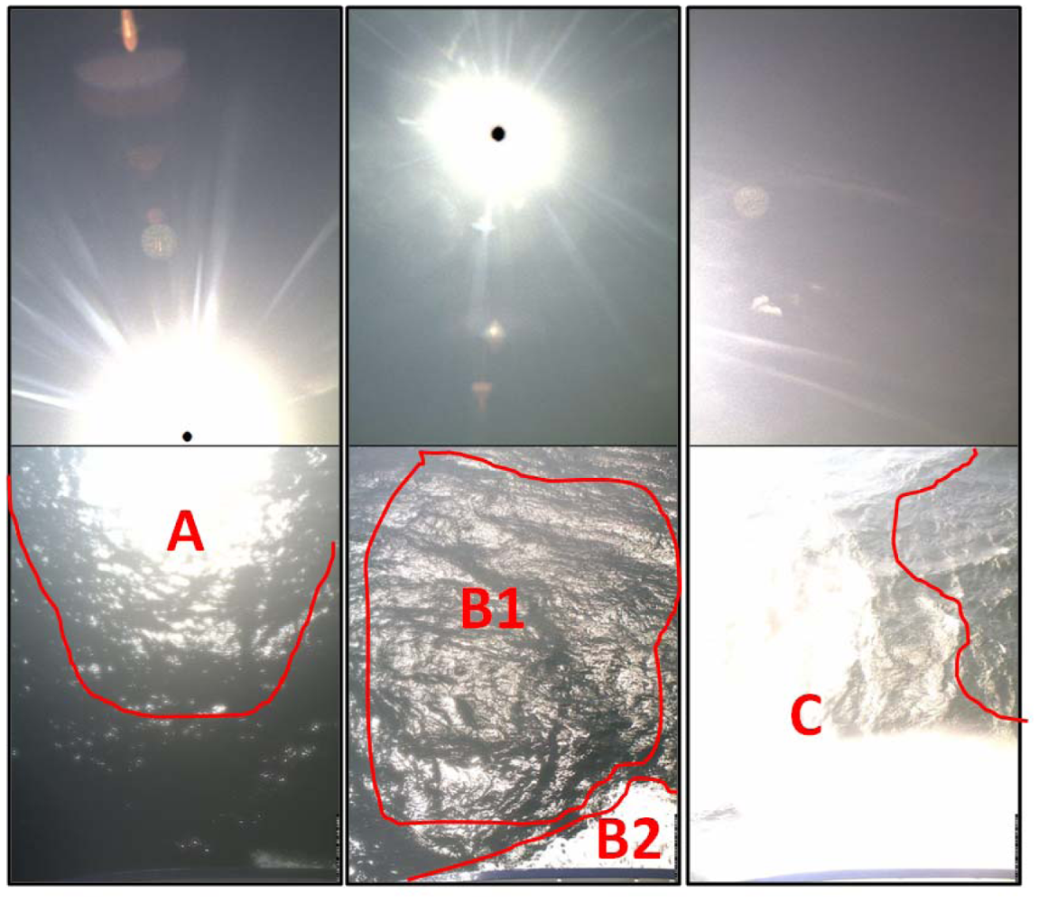
Automated and unmanned optical measurements from a seaborne platform are challenging. It is difficult to adhere to recommended sensor setups for θ_sfc, θ_sky, Φ; thus it is inevitable to collect measurements affected by sunglint, whitecap and foam [18–20]. Figure 5 demonstrates typical situations also noted during the image inspection in step 2 [Section 2.2.1 and Figure 3(a,b)].

Using the automated sunglint image detection algorithm, the output was either an image with a probability of sunglint or without. Sunglint (Figure 5(A,B1,C)) as well as whitecaps and foam (Figure 5(B2,C)) were identified as main sources of contamination, with the latter two presumably resulting in similar sunlight influenced spectral patterns. This image algorithm detects overexposure which is a result of sunglint and/or whitecaps and foam; we however assume that sunglint plays a major role.

3.2. Sunglint Flag

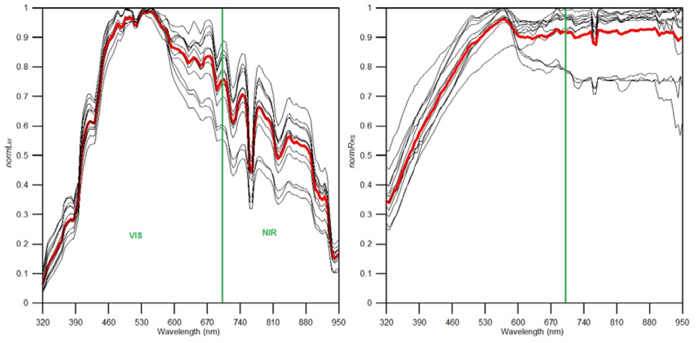
A spectral assessment of the sample sets indicated that R_RS (NIR) and L_W (NIR) are significantly enhanced for Ns, compared to Nns. The enhanced spectra in set Ns were assumed to be a result of sunglint, whitecaps, and foam. In Figure 6 normalised mean spectral shapes for Nns (501 spectra) and Ns (128 spectra) illustrate these findings. Data normalisation was applied to simplify the visual comparison of spectra, dividing each L_W (λ) and R_RS (λ) measurement by the maximum value for each measurement. However, for determining the flagging criteria, the actual computed spectral measurements L_W (λ) and R_RS (λ) were used.

Figure 6 shows how the mean spectra, with respect to normL_W and normR_RS values, are enhanced in the presence of sunglint in both the VIS and NIR compared to the non-sunglint situation. To further investigate sunglint spectral characteristics, 13 of the 128 sea surface images in Ns were identified to be highly affected by sunglint (see Figure 7). Their spectral shapes also reveal the same trend of enhanced water leaving and reflectance signal over the measured spectrum.

Spectral band ratios, a conventional approach in remote sensing algorithms, were implemented to identify differences in Nns and Ns. In previous reports related to sunglint correction, the following characteristic spectral bands were used mainly due to their physical properties: (a) oxygen absorption band (λ ≈ 760 nm) which has been used in a prior sunglint correction model [21]; (b) water and precipitable water vapour absorption band (λ ≈ 940 nm) known to interact with solar radiation in the NIR [17,22]; and (c) coloured dissolved organic matter absorption from UV to visible, here investigated at (λ ≈ 400 nm) and (λ ≈ 460 nm), contributing to sunglint through multiple scattering [23,24].

Several tests were implemented to obtain the most effective sunglint flagging. Test results are summarized in Table 1. A ranking was introduced grouping the methods according to their performance in the detection of sunglint affected data.

The method of thresholds was chosen because it is a widely used technique in developing flagging and validation algorithms [13,25,26]. Another benefit of using a threshold is the possibility of adjusting them to improve sensitivity of algorithms or models [27]. The threshold values were obtained by repetitive testing of possible threshold values i.e., after statistically computing the min, max and mean for spectra in the NIR. The computed statistics provided a starting test point and altered to obtain the best threshold values aimed at; (i) masking/eliminating as many measurements in the sunglint-affected set Ns; and (ii) unmasking/keeping as many measurements in the sunglint free set Nns. The performance test summarized in Table 1, revealed the most effective sunglint flagging criteria if the effectiveness of both tasks is taken into account;

‘mean (L_W)_NIR < 2 mW·m⁻²·nm⁻¹·Sr⁻¹’, being 97% effective in sets Nns and 91% effective in Ns (91%); Or alternatively

‘minimum (R_RS)_NIR < 0.010 Sr⁻¹’, with an effectiveness of 95% in sets Nns and 94% in Ns.

3.3. Remote Sensing Reflectance

In the previous section, a sunglint flagging was identified which can be implemented using either L_W or R_RS. Both, the meteorological flagging conditions [13] and herein proposed sunglint flag criteria are presented in Table 2. The first three flags rely on the incoming radiation, E_s, thus masking measurements taken during dusk or with too low incoming solar radiation (Flag 1), during dawn (Flag 2), or under rainfall (Flag 3). Equation 1 is then applied to derive the water leaving radiance, L_W and remote sensing reflectance, R_RS, followed by the sunglint flag validation. In this study the sunglint flag was implemented using L_W (Flag 4a) because it is the first product of Equation 1 but can be replaced by R_RS (Flag 4b) as summarised in Table 2. In order not to limit flagging to one remote sensing product, e.g., L_W or R_RS only, Flag 4a or Flag 4b were proposed.

4. Conclusions and Outlook

In this study we developed two alternative sunglint flagging criteria as a quality control procedure for unmanned and automated above-water platforms measuring water reflectance. To provide an independent evaluation method for sunglint situations, an automated sunglint image detection algorithm was successfully implemented. The Flag 1 (the minimal E_S accepted) is a bit arbitrary and certainly depends on the geographical position. Flag 2 can be discussed, although this flag does not depend on the region but more or less on sun rise and fall. We choose for a more or less average shaped spectrum (comparable with the form of the Es spectrum at high noon, only amplitude differs. Flag 4 is depends on the region as we are using a empirical approach and therefore makes the use of the camera important.

We assumed sunglint to be the main cause of error in the collected measurements after applying the meteorological flagging [13]. However, the influence of whitecaps and foam has been reported to cause both: (i) a decrease in reflectance in the NIR due to radiation absorption by large air bubbles [28,29], or physical coolness of residual foam [30]; (ii) enhanced reflectance occurring as soon as waves break generating thick strong reflecting foam [20]. The image analysis revealed that sunglint was also present in sea surface images influenced by whitecaps/foam, and it was not possible to distinguish how each of them contributes to the spectra. It was therefore assumed that for the available measurements sunglint and whitecaps/foam led to contaminated measurements. It is for this reason that in future studies the contribution of whitecaps and foam be specifically investigated with respect to sunglint flagging, possibly utilising novel glint measurement apparatus e.g., [31,32] integrated with sunglint and wave models such as [4,5,7,15,33].

The sunglint image detection algorithm introduced here has shown to be a valuable additional tool for detecting contaminated sensor readings. However, the used values for T_L and T_U are empirical. Results with the given values have shown a good congruence with visual inspection by a human investigator. It might useful to adjust thresholds to specific situations or locations. Higher counts in the bright part of the histogram result in the situation that the ‘target’ line intersects the x-axis at higher values. Thus, increased numbers of bright pixels simultaneously emphasize the shape of the histogram on the ‘bright side’. Using different values for T_L and T_U impacts the sensitivity of the function for darker/brighter pixels.With respects to sensor setup we suggest that prior to automated and unmanned optical measurements the Solar Position Algorithm [34] be utilised to predict or identify optimal relative angle of optical sensor setup to the sun's position despite the limiting factors of R/V pitch, roll and yaw motions [14,18,35]. Here the idea is not to necessarily change the cruise track but to perform underway optical measurements avoiding sunglint. Alternative approaches to minimise sunglint, but increasing technical requirements, would be (a) to turn the sensors by some automatic device e.g., RFlex (http://www.sourceforge.net/p/rflex/wiki/Home/) or (b) to have more sensors and cameras looking at different azimuthal directions. However for fixed platforms, such as piles, these alternative approaches can be avoided if SPA is utilised beforehand to limit sunglint influenced measurements. Furthermore, we provide a set of step that can be followed to perform sunglint correction on above-water automated measuring platforms (Appendix A).

Recently operational oceanographic observatories are becoming more prominent and at the same time hyperspectral radiance sensor technology becomes increasingly affordable [2,3]. Therefore the application of reflectance measurements above the water surface, from stationary and moving platforms alike, is expected to significantly grow in numbers. Given this enormous amount of data, favourably processed in real-time, effective quality control procedures like the ones discussed here are more than supporting tools, they are a crucial prerequisite for trustworthy and manageable information.

The authors extend their gratitude to the master and crew of R/V Heincke, and to R. H. Henkel, B. Krock, B. Saworski and D. Voβ for their support during the field campaign. This work was supported by Institute of Marine Resources (IMARE) GmbH subsidised by European Regional Development Fund (ERDF), University of Applied Science Bremerhaven and Coastal Observation System for Northern and Arctic Seas (COSYNA).

Appendix A

The following recommendations assume automated and unmanned platform above-water radiometry is performed using the setup explained in this report. For a detailed explanation of the correction models refer to the respective protocols.

Prerequisite information: -

Wind speed [m/s]

Cloud cover

○

L_sky(750)/E_s(750) [15]

■

<0.05 means clear sky

■

≥0.05 means cloudy sky

Ship heading

Ship GPS data

Sea surface images

Step 1

Apply three meteorological flags:

E_S (λ = 480 nm) > 20 mW·m⁻²·nm⁻¹ setting a threshold for which significant E_S (λ) can be measured.

E_S (λ = 470 nm)/E_S (λ = 680 nm) < 1 masking spectra affected by dawn/dusk radiation.

E_S (λ = 940 nm)/E_S (λ = 370 nm) < 0.25 masking spectra affected by rainfall and high humidity [13].

Step 2 Alternative 1

Usage of the collected sea surface images and implementation of the sunglint detection algorithm. It eliminates images too contaminated with sunglint. Respective matching spectra of images successfully passing the image detection algorithm are used in Step 3.

Alternative 2

Determine L_W and R_RS and apply the spectral conditions supplied for sunglint flagging. To validate and verify flagging performance cross check with the image algorithm.

If not satisfactory, follow the procedures described in Section 2.2.2. ‘Spectral Analysis for Sunglint Flag’ and adjust the sunglint flag conditions appropriately.

Alternative 3

Determine the relative azimuthal angle of the sensor to the sun using e.g., Solar Position Algorithm, SPA [34]. Using the ship's position the SPA will compute the sun's azimuthal and zenith angle at a given space-time spot.

Extract spectra collected in the optimal relative azimuthal angle of sensor to sun 90° ≤ Φ ≤ 135°.

In this case if required, verify measurements with the image sunglint detection algorithm to further eliminate images with too much glint or above average white pixels.

Proceed with next step.

Step 3—Sunglint Correction

To determine which coefficient optimally removes sea surface reflectance/sunglint a number of methods are available. It is important to test them and decide on which correction model to apply from these:

Lee <italic>et al.</italic> [<xref ref-type="bibr" rid="b4-sensors-12-12545">4</xref>]

Lee et al., recommends a spectral optimization where ρ_air-sea = 0.022 = Fresnel Reflectance. Additionally a bias delta (Δ), obtained from comparing modeled R_RS and in-situ R_RS, is then used as residual sea surface reflectance. To calculate R_RS use Equation (2): (2) R R S = L sfc E S − ρ air − sea ⋅ L sky E S − Δ

Ruddick <italic>et al.</italic> [<xref ref-type="bibr" rid="b15-sensors-12-12545">15</xref>]

Ruddick et al., provides a model based on cloud cover and wind speed, W that is aimed at correcting sunglint for measurements from turbid to very turbid water, to calculate R_RS use Equation (3).

L_sky(750)/E_d(750) test for presence of cloud cover in L_sky field of view [15]

○

<0.05 means clear sky ρ_air-sea = 0.0256 + 0.00039 W + 0.000034 W²

○

≥0.05, cloudy sky ρ_air-sea = 0.0256 (3) R R S = L W E S = L sfc − ( ρ air − sea ⋅ L sky ) E S

Gould <italic>et al.</italic> [<xref ref-type="bibr" rid="b5-sensors-12-12545">5</xref>]

According to Gould et al. [5] correction can be performed for sunglint by assuming that sunglint consists of (a) spectrally variable sky radiance ρ_air-sea (0.021) × L_sky and (b) spectrally-flat sunglint and cloud reflected radiance, B. To calculate R_RS use Equation (4): (4) R R S = L sfc E S − ρ air − sea ⋅ L sky E S − B

Mobley [<xref ref-type="bibr" rid="b8-sensors-12-12545">8</xref>]

Mobley provides a number of simulations and recommends ρ_air-sea = 0.028 for clear skies and wind speed < 5 m/s. For higher wind speeds change adjust ρ_air-sea accordingly. For cloudy skies at all wind speeds he recommends ρ_air-sea = 0.028. However, take note that the higher the ρ_air-sea is you might over correct and get negative reflectance in the NIR. To calculate R_RS use Equation (5): (5) R R S = L W E S = L sfc − ( ρ air − sea ⋅ L sky ) E S

References 1.

International Ocean Colour Coordinating Group (IOCCG)

Remote Sensing of Ocean Colour in Coastal, and Other Optically-Complex, WatersSathyendranath

IOCCG

Dartmouth, NS, Canada

2000 2.

Moore

Barnard

Fietzek

Lewis

M.R.

Sosik

H.M.

White

Zielinski

Optical tools for ocean monitoring and research

Ocean Sci.20095661684

10.5194/os-5-661-2009

Glenn

Schofield

Dickey

T.D.

Chant

Kohut

Barrier

Bosch

Bowers

Creed

Halderman

The expanding role of ocean color and optics in the changing field of operational oceanography

Oceanography2004178695

10.5670/oceanog.2004.52

Lee

Ahn

Y.-H.

Mobley

Arnone

Removal of surface-reflected light for the measurement of remote-sensing reflectance from an above-surface platform

Opt Express2010182631326324

10.1364/OE.18.026313

21164981

Gould

R.W.

Arnone

R.A.

Sydor

Absorption, scattering, and, remote-sensing reflectance relationships in coastal waters: Testing a new inversion algorithm

J. Coast. Res.200117328341 6.

Zhang

Wang

Evaluation of sun glint models using MODIS measurements

J. Quant. Spectrosc. Radiat. Transf.2010111492506

10.1016/j.jqsrt.2009.10.001

Cox

Munk

Measurement of the roughness of the sea surface from photographs of the sun's glitter

J. Opt. Soc. Am.195444838850

10.1364/JOSA.44.000838

Mobley

C.D.

Estimation of the remote-sensing reflectance from above-surface measurements

Appl. Opt.19993874427455

10.1364/AO.38.007442

18324298

Kay

Hedley

Lavender

Sun glint correction of high and low spatial resolution images of aquatic scenes: A review of methods for visible and near-infrared wavelengths

Remote Sens.20091697730

10.3390/rs1040697

10.

Siegel

D.A.

Wang

Maritorena

Robinson

Atmospheric correction of satellite ocean color imagery: The black pixel assumption

Appl. Opt.20003935823591

10.1364/AO.39.003582

18349929

11.

Shi

Wang

An assessment of the black ocean pixel assumption for MODIS SWIR bands

Remote Sens. Environ.200911315871597

10.1016/j.rse.2009.03.011

12.

Jamet

Loisel

Kuchinke

C.P.

Ruddick

Zibordi

Feng

Comparison of three SeaWiFS atmospheric correction algorithms for turbid waters using AERONET-OC measurements

Remote Sens. Environ.201111519551965

10.1016/j.rse.2011.03.018

13.

Wernand

M.R.

Guidelines for (Ship-Borne) Auto-Monitoring of Coastal and Ocean Colour

Proceedings of Ocean Optics XVI

Santa Fe, NM, USA

18– 22 November 2002

Ackleson

S.G.

Trees

13 14.

Mueller

J.L.

Davis

Arnone

Frouin

Carder

Lee

Z.P.

Steward

R.G.

Hooker

Mobley

C.D.

McLean

Above-Water Radiance and Remote Sensing Reflectance Measurement and Analysis ProtocolsGoddard Space Flight Space Center

Greenbelt, MD, USA

2003 15.

Ruddick

K.G.

de Cauwer

Park

Y.J.

Moore

Seaborne measurements of near infrared water-leaving reflectance: The similarity spectrum for turbid waters

Limnol. Oceanogr.20065111671179

10.4319/lo.2006.51.2.1167

16.

Doxaran

Babin

Leymarie

Near-Infrared light scattering by particles in coastal waters

Opt Express2007151283412849

10.1364/OE.15.012834

19550552

17.

Halthore

R.N.

Eck

T.F.

Holben

B.N.

Markham

B.L.

Sun photometric measurements of atmospheric water vapor column abundance in the 940-nm band

J. Geophys. Res.199710243434352

10.1029/96JD03247

18.

Hooker

S.B.

Morel

Platform and environmental effects on above-water determinations of water-leaving radiances

J. Atmos. Ocean. Technol.200320187205

10.1175/1520-0426(2003)020<0187:PAEEOA>2.0.CO;2

19.

Fougnie

Frouin

Lecomte

Deschamps

P.-Y.

Reduction of skylight reflection effects in the above-water measurement of diffuse marine reflectance

Appl. Opt.19993838443856

10.1364/AO.38.003844

18319991

20.

Moore

K.D.

Voss

K.J.

Gordon

H.R.

Spectral reflectance of whitecaps: Instrumentation, calibration, and performance in coastal waters

J. Atmos. Ocean. Technol.199815496509

10.1175/1520-0426(1998)015<0496:SROWIC>2.0.CO;2

21.

Kutser

Vahtmäe

Praks

A sun glint correction method for hyperspectral imagery containing areas with non-negligible water leaving NIR signal

Remote Sens. Environ.200911322672274

10.1016/j.rse.2009.06.016

22.

Kleidman

R.G.

Kaufman

Y.J.

Gao

B.C.

Remer

L.A.

Brackett

V.G.

Ferrare

R.A.

Browell

E.V.

Ismail

Remote sensing of total precipitable water vapor in the near-IR over ocean glint

Geophys. Res. Lett.20002726572660

10.1029/1999GL011156

23.

Bricaud

Morel

Prieur

Absorption by dissolved organic matter of the sea (yellow substance) in the UV and visible domains

Limnol. Oceanogr.1981264353

10.4319/lo.1981.26.1.0043

24.

Gallegos

C.L.

Correll

D.L.

Pierce

J.W.

Modeling spectral diffuse attenuation, absorption, and scattering coefficients in a turbid estuary

Limnol. Oceanogr.19903514861502

10.4319/lo.1990.35.7.1486

25.

Wang

Jiang

Study on the seasonal variation of the suspended sediment distribution and transportation in the East China Seas based on SeaWiFS data

J. Ocean Univ China (English Edition)20087385392 26.

Lavender

S.J.

Pinkerton

M.H.

Moore

G.F.

Aiken

Blondeau-Patissier

Modification to the atmospheric correction of SeaWiFS ocean colour images over turbid waters

Cont. Shelf Res.200525539555

10.1016/j.csr.2004.10.007

27.

Freeman

E.A.

Moisen

G.G.

A comparison of the performance of threshold criteria for binary classification in terms of predicted prevalence and kappa

Ecol. Model.20082174858

10.1016/j.ecolmodel.2008.05.015

28.

Whitlock

C.H.

Bartlett

D.S.

Gurganus

E.A.

Sea foam reflectance and influence on optimum wavelength for remote sensing of ocean aerosols

Geophys. Res. Lett.19829719722

10.1029/GL009i006p00719

29.

Frouin

Schwindling

Deschamps

P.-Y.

Spectral reflectance of sea foam in the visible and near-infrared: In situ measurements and remote sensing implications

J. Geophys. Res.19961011436114371

10.1029/96JC00629

30.

Marmorino

G.O.

Smith

G.B.

Bright and dark ocean whitecaps observed in the infrared

Geophys. Res. Lett.200532L11604

10.1029/2005GL023176

31.

Ottaviani

Stamnes

Koskulics

Eide

Long

S.R.

Wiscombe

Light reflection from water waves: Suitable setup for a polarimetric investigation under controlled laboratory conditions

J. Atmos. Ocean. Technol.200825715728

10.1175/2007JTECHA1049.1

32.

Ottaviani

Merck

Long

Koskulics

Stamnes

Wiscombe

Time-resolved polarimetry over water waves: Relating glints and surface statistics

Appl. Opt.20084716381648

10.1364/AO.47.001638

18385775

33.

Munk

An inconvenient sea truth: Spread, steepness, and skewness of surface slopes

Annu. Rev. Marine Sci.20091377415

10.1146/annurev.marine.010908.163940

34.

Reda

Andreas

Solar position algorithm for solar radiation applications

Sol Energy200476577589

10.1016/j.solener.2003.12.003

35.

Hooker

S.B.

Zibordi

Platform perturbations in above-water radiometry

Appl. Opt.200544553567

10.1364/AO.44.000553

15726953

Figures and Tables Figure 1.

R/V Heincke HE302 cruise track (red line) where above-water hyperspectral optical measurements were taken between 21 April and 14 May 2009.

Figure 2.

Optical sensor and camera system setup on the mast of R/V Heincke. Highlighted in red on the left side is the RAMSES hyperspectral radiometers setup, and on the right side is the DualDome D12 camera system with a sample set of captured sky and sea surface images, not to scale.

Figure 3.

Schematic diagram of the automated sunglint image detection algorithm. (A) Cropping original sea surface image; (B) Converting cropped image to greyscale; (C) Extract grey level histogram of cropped and converted image; (D) Define lower (T_L) and upper (T_U) threshold; (E) Find position and magnitude of local maxima of darker (x_TL, y_TL) and brighter (x_TU, y_TU) colours and calculate slope of line segment; (F–G) Calculate midpoint (mid_x, mid_y) of line segment between (x_TL, y_TL) and (x_TU, y_TU); (H) Calculate slope and intercept of the target line being perpendicular to the previously calculated slope line crossing the midpoint (mid_x, mid_y); (I) Calculate target line's crossing with abscissa. If and only if this value is larger than T_U, the image is tagged as probably overexposed.

Figure 4.

A simplified activity diagram showing the four steps involved in generating the new sunglint flag. (1) Automated sunglint image detection and sorting of spectra into Nns–image set without sunglint or Ns–sunglint-affected image set; (2) Analysis of the two spectra sets (λ = 320–950 nm); (3) Specific spectra analysis in visible λ = 320–700 nm and near infra-red λ = 700–950 nm range (4) Performance test and identification of effective sunglint flagging criteria.

Figure 5.

Starboard side sky (top) and sea surface (bottom) images captured during R/V Heincke field campaign HE302 showing sources of erroneous measurements; (A)—sunglint; (B1)—sunglint and (B2)—whitecap or foam; and (C)—a combination of sunglint, whitecaps and foam.

Figure 6.

Normalised mean spectral shapes for the sunglint free set Nns (top) and sunglint set Ns (bottom). The green line highlights the spectral limits for the VIS (λ = 320–700 nm) and NIR (λ = 700–950 nm).

Figure 7.

Thirteen samples of spectral shapes for sea surface images strongly affected by sunglint from the sunglint image set Ns. On the left is the normalized water leaving radiance, normL_W and on the right is the normalized remote sensing reflectance, normR_RS. It is observed that sunglint enhances the measured signal especially in the NIR for both water leaving and remote sensing reflectance. The red spectrum shows the mean spectral shape and the green line highlights the VIS and NIR spectral ranges.

Table 1.

A summarized evaluation of the most effective sunglint flagging ranked according to their performance in masking sunglint spectra in a reanalysis. To check for effectiveness, the percentage E (Ns) % and E (Nns) % was derived by dividing the number of spectra masked or unmasked by each condition with the actually number of spectra in sets (sunglint set Ns—128 spectra and non sunglint set Nns—501 spectra).

Sunglint Flag Test Condition	Sunglint Affected Observations Masked	E (Ns) %	Sunglint Free Observations Unmasked	E (Nns) %
Minimum (L_W)_NIR < 0.3 mW/m²·nm·Sr	123	96	454	91
Mean (R_RS)_NIR < 0.010 Sr⁻¹	123	96	453	90
Minimum (R_RS)_NIR < 0.010 Sr⁻¹	121	95	471	94
Minimum (L_W)_NIR < 0.4 mW/m²·nm·Sr	119	93	478	95
Mean (L_W)_NIR < 2.000 mW/m²·nm·Sr	117	91	487	97
Minimum (L_W)_NIR < 0.5 mW/m²·nm·Sr	115	90	486	97
Minimum (R_RS)_NIR < 0.012 Sr⁻¹	115	90	479	96
Mean (R_RS)_NIR < 0.015 Sr⁻¹	112	88	475	95
L_W (940)/L_W (400) < 0.145	111	87	480	96
Mean (L_W)_NIR < 2.500 mW/m²·nm·Sr	110	86	492	98
L_W (765)/L_W (460) < 0.290	110	86	477	95
Minimum(R_RS)_NIR < 0.015 Sr⁻¹	109	85	490	98
R_RS (765)/R_RS (400) < 0.700	109	85	468	93
R_RS (760)/R_RS (400) < 0.700	108	84	470	94
L_W (940)/L_W (460) < 0.090	108	84	488	97
R_RS (760)/R_RS (460) < 0.650	107	84	473	94

Table 2.

Summarised meteorological and sunglint flag conditions. The meteorological criteria [13] are represented by Flags 1–3. The sunglint flag can be implemented either as Flag 4a or Flag 4b depending on availability of measured water leaving radiance, L_W or remote sensing reflectance, R_RS.

Flag Name	Purpose	Test Conditions
Flag 1	The ‘minimal flag’ sets the lower limit for which significant incoming solar radiation can be measured.	E_s (480 nm) > 20 mW/m² nm
Flag 2	The ‘shape flag’ will mask optical measurements influenced by dusk ‘red colouring of the sky’ or dawn radiation.	E_s (470 nm)/E_s (680 nm) < 1
Flag 3	The ‘rainfall flag’ will mask optical measurements influenced by precipitation or high humidity.	E_s (940 nm)/E_s (370 nm) > 0.25
Flag 4a	The ‘sunglint flag’ will mask optical measurements influence by sunglint based on L_W.	Mean L_w (700–950 nm) < 2 m W/m² nm Sr
Flag 4b	Alternative ‘sunglint flag’ based on R_RS.	Minimum R_RS (700–950 nm) < 0.010 Sr⁻¹