Analysis of Airborne Particulate Matter (PM2.5) over Hong Kong Using Remote Sensing and GIS


Abstract
: Airborne fine particulates (PM2.5; particulate matter with diameter less than 2.5 μm) are receiving increasing attention for their potential toxicities and roles in visibility and health. In this study, we interpreted the behavior of PM2.5 and its correlation with meteorological parameters in Hong Kong, during 2007–2008. Significant diurnal variations of PM2.5 concentrations were observed and showed a distinctive bimodal pattern with two marked peaks during the morning and evening rush hour times, due to dense traffic. The study observed higher PM2.5 concentrations in winter when the northerly and northeasterly winds bring pollutants from the Chinese mainland, whereas southerly monsoon winds from the sea bring fresh air to the city in summer. In addition, higher concentrations of PM2.5 were observed in rush hours on weekdays compared to weekends, suggesting the influence of anthropogenic activities on fine particulate levels, e.g., traffic-related local PM2.5 emissions. To understand the spatial pattern of PM2.5 concentrations in the context of the built-up environment of Hong Kong, we utilized MODerate Resolution Imaging Spectroradiometer (MODIS) Aerosol Optical Thickness (AOT) 500 m data and visibility data to derive aerosol extinction profile, then converted to aerosol and PM2.5 vertical profiles. A Geographic Information Systems (GIS) prototype was developed to integrate atmospheric PM2.5 vertical profiles with 3D GIS data. An example of the query function in GIS prototype is given. The resulting 3D database of PM2.5 concentrations provides crucial information to air quality regulators and decision makers to comply with air quality standards and in devising control strategies.1. Introduction
Airborne Particulate Matter (PM) refers to particles suspended in the air in either liquid or solid form, which are highly heterogeneous in both time and space and are often observable as dust, smoke and haze. PM2.5 and PM10 are defined as particles with diameters of 2.5 μm or less, and 10 μm or less respectively, they are the standard concentrations used in the United States Environmental Protection Agency (EPA). Aerosol is defined as the total particles suspended in air with typical particle radius ranged from 0.05 to 15 μm [1]. Around 10% of the aerosols is produced by or is a result of human activities such as vehicular exhaust, burning of fossil fuel, construction, while the remaining 90% is produced by natural sources such as volcanic eruptions, sea spray and dust [2,3]. The scattering and absorption of light by the aerosol particles results in a degradation of visibility [4]. Satellite aerosol remote sensing provides Aerosol Optical Thickness (AOT) data, as a quantitative measurement of PM loadings in the atmosphere column [5]. To some extent, the AOT can be seen as an important indicator of air pollution and is the most readily recognized indication of the presence of particulate air pollution.
Airborne particulates can be inhaled by the human lungs, where they are absorbed into blood, and consequently are responsible for harmful health effects. The significance of adverse effects on our health depends on the size and composition of particulates. For instance, particles less than 2.5 μm (PM2.5) can penetrate deeper into the air sacs of human lungs and therefore pose the greatest harm to human health [6]. Environmental epidemiological studies have found particulate matters affect pulmonary function and can thereby induce respiratory diseases and adverse effects on public health and even premature death [7–9].
Elevated levels of PM2.5 over urban areas are often associated with both local sources of emissions and regional transport [10]. Although diesel vehicles are the main local sources of urban PM2.5 loads [11], regional transport and secondary transformation also account for a significant portion of PM2.5 levels. Numerous studies have been conducted to link the behavior of PM2.5 to meteorological data e.g., wind speed, wind direction, temperature, humidity, mixing height, precipitation, pressure and cloud cover [12,13]. Jung et al. [14] studied the atmospheric transport of PM2.5 in Ohio, United States, and found high concentrations of PM2.5 were particularly detected when the wind speeds were lower than 8 mph and the temperature was higher than 70 °F. Hien et al. [15] revealed that the fine particles were governed mainly by wind speed and temperature. Chiang et al. [16] found wind direction and relative humidity are highly correlated to fine particulates in winter.
Due to the temporal and spatial dependence of the pollutant, the characteristics of PM2.5 resolved in one region cannot be replicated to another region. Although there are some existing PM2.5 studies in Hong Kong [17–19], they are mainly focused on the chemical composition and only a few studies link pollutant characteristics to the meteorological parameters such as wind effects [20]. The extensive and comprehensive meteorology contribution to PM2.5 loadings is poorly understood in Hong Kong. Since understanding the pattern of pollutant and quantifying the relative contribution of different meteorological parameters are critical in developing control and mitigation strategies to safeguard public health, a detailed analysis of the temporal pattern of PM2.5 and the related meteorological contribution is imperative in Hong Kong. Thus, the objective of this study is to assess temporal and spatial patterns of PM2.5 in Hong Kong. The temporal variations of PM2.5 over urban areas in Hong Kong will be analyzed using ground-based data (meteorological and PM2.5 data), while the spatial patterns of PM2.5 will be derived from remote sensing and GIS approaches.
2. Data Collection
2.1. PM2.5 and Meteorological Measurements
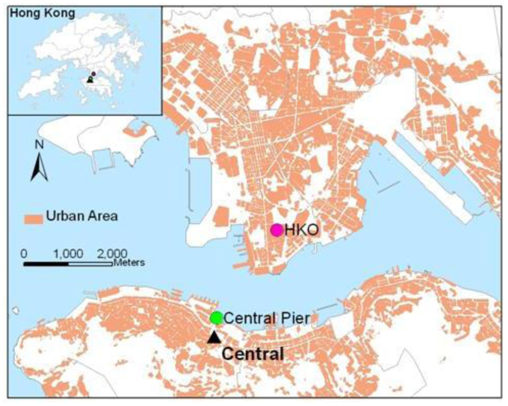
To characterize and analyze the PM2.5 concentrations in Hong Kong, the PM2.5 concentrations and meteorological data were acquired from the Hong Kong Environment Protection Department (HKEPD) and the Hong Kong Observatory (HKO) respectively. In this study, PM2.5 data recorded by Central station (22°16′54″, 114°09′29″) equipped with a TEOM Series 1400a monitor [21] are selected to represent PM2.5 concentrations over urban areas in Hong Kong. These data are represented for the pollution in Central Business District and are considered to have higher values than suburban and rural areas. Temperature, relative humidity, pressure, and precipitation were collected from the HKO (22°18′07″, 114°10′27″), which were used to represent the meteorological conditions for Central station (Figure 1). The wind speed and wind direction were collected from Central Pier monitoring station (22°17′20″, 114°09′21″) for representing the wind conditions for Central station as geographical proximity. These data are co-located in both space and time, which serve as the basis for statistical analysis.
2.2. MODIS AOT 500 m Image
The MODerate Resolution Imaging Spectroradiometer (MODIS) is a sensor aboard the TERRA and AQUA Earth observation system satellites. It is a multispectral (36 spectral wavebands span over the visible light, near infrared and infrared portion of the spectrum), multi-resolution (1 km, 500 m, 250 m) sensor dedicated to the observation of the Earth. However the coarse spatial resolution (10 × 10 km) of MODIS Aerosol Optical Thickness (AOT), namely MOD04 aerosol product [22] cannot provide detailed spatial variation for local/urban scale aerosol monitoring and is inaccurate over bright urban surfaces [23], Wong et al. [23,24] developed a modified Minimum Reflectance Technique (MRT) to derive AOT over both bright and dark surfaces (e.g., urban and vegetated areas) at the relatively high resolution of 500 m, for Hong Kong and the Pearl River Delta regions.
3. Methodology
3.1. Analyzing PM2.5 with Meteorological Data
In order to understand the interrelationship between PM2.5 and meteorological parameters, the correlations between them were first calculated. The diurnal patterns of PM2.5 concentration and meteorological data were also studied to understand their influences during summer and winter time. In addition, seasonal variations of PM2.5 as well as meteorological parameters were studied. The daily concentrations (24 hour average) of PM2.5 and meteorological parameters of 2007 and 2008 were calculated from the hourly data and then grouped into each season such as spring (March–May), summer (June–August), autumn (September–November) and winter (December–February).
3.2. Modeling PM2.5 Data with AOT Data
In contrast to ground level PM2.5 measurement, satellite remote sensing provides aerosol optical thickness to study urban air pollution with broad spatial coverage [25]. AOT is found to be dominated by near-surface emission except for long range dust events [26]. Recent studies have established quantitative relationships between MODIS derived AOT and PM2.5 using linear regression models. Wang and Christopher [27] achieved a correlation coefficient of 0.7 between satellite-derived AOT at 550 nm and PM2.5 measured at seven locations in Alabama, United States. Wong et al. [28] showed a good correlation between MODIS derived 500 m AOT and PM2.5 (r2 = 0.67), which demonstrated great potential for MODIS derived 500 m AOT as a good surrogate for PM2.5 monitoring. In this study, we attempted to model the 2D (image) and vertical distributions of PM2.5 which has not been done in any other study. The resulting 3D database of PM2.5 concentrations can be used for daily air quality monitoring in environmental authority. First, the aerosol extinction profile (σa(z)) was modeled and the columnar AOT was divided into AOTΔz at different elevations [29,30]. Then by utilizing the equation (PM2.5 = 63.66 × AOT + 26.56) developed by Wong et al. [28], the PM2.5Δz at different elevations can be derived.
By integrating the extinction coefficient profile on two different elevations z1 and z2, AOTΔz between two elevations (Δz) can be computed [31] (note: Δz = z2 − z1):
The aerosol scaling height z0 is defined as the height of an exponential profile at which the value is decreased by 1/e from the ground level value σa(z0). It describes the decreasing rate of AOT with altitude and can be calculated using Equation (2) [32,33]:
Given the surface extinction coefficient σa(z0), and insignificances of the aerosol hygroscopic growth effect when relative humidity is less than 70% [35,36], the vertical extinction profile can be estimated:
The whole columnar AOT can be divided to AOTΔz by assigning any two given heights (Δz) in Equation (1):
In a similar way, visibility at any height Visz can be calculated from the extinction coefficient by inverting the Koschmeider equation (Equation (3)).
Finally, PM2.5Δz concentrations at different elevations can be estimated by applying the linear regression equation (PM2.5 = 63.66 × AOT + 26.56) developed by Wong et al. [28]:
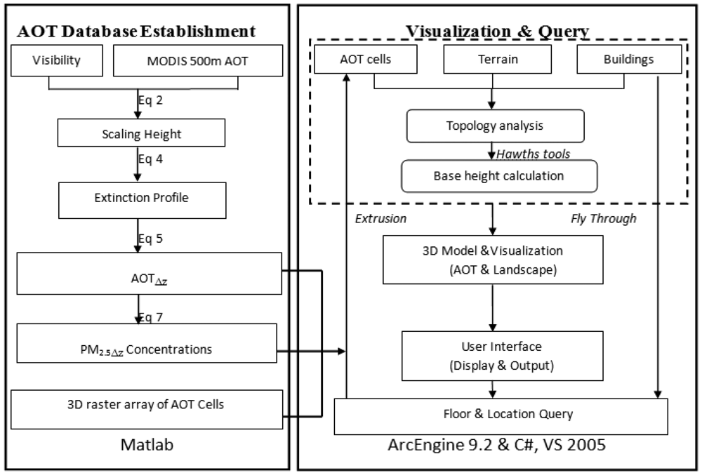
A program code in Matlab has been developed for data matching and converting AOT to PM2.5Δz. Another program written in ArcEngine helps to display and visualize the data in 3D. The work flow of these programs is shown in Figure 2.
4. Results
4.1. Correlation between PM2.5 Data with Meteorological Data
Table 1 shows the interrelationship between PM2.5 and meteorological parameters over Hong Kong on a daily average basis. Moderate correlations were observed between PM2.5 and temperature (TEMP), relative humidity (RH), and mean sea level pressure (MSLP), and fair correlations were observed from the other two parameters: wind speed (WS), wind direction (WD).
4.2. Diurnal Trend of PM2.5 Concentration and Meteorological Data
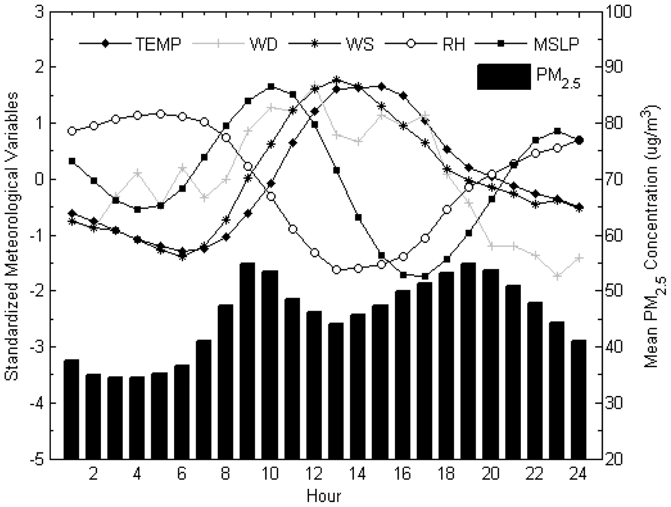
Figure 3 showed the diurnal trends of PM2.5 and meteorological parameters. PM2.5 showed a distinctive diurnal pattern while low values observed during night time (01:00–05:00). During the daytime, PM2.5 exhibited a bimodal pattern with two marked peaks, during morning rush hours (08:00–10:00) and evening rush hours (18:00–20:00), typically when high traffic density occur. Similar observations and implications were reported by Chan and Kwok [37].
Wind direction does not show a clear diurnal pattern. Mean sea level pressure has a similar pattern to that of PM2.5 in spite of the time lag, which displayed two clear maxima around 10:00 and 23:00. In contrast, temperature and wind speed exhibit a unimodal pattern characterized by midday maxima around 13:00. Relative humidity, however, exhibits an inverse unimodal pattern with stable overnight maximum values, which suggests the negative association with nocturnal PM2.5 concentrations. A high relative humidity can depress the absorption of gas phase organic species into particle surface [38] and accelerate the removal of particle by dry deposition, this mechanism enhanced for hygroscopic particle [39]. Thus, PM2.5 keeps constant at minimum values between 02:00 and 05:00. Another reason is due to less influence of anthropogenic activities on fine particulate levels during nighttime.
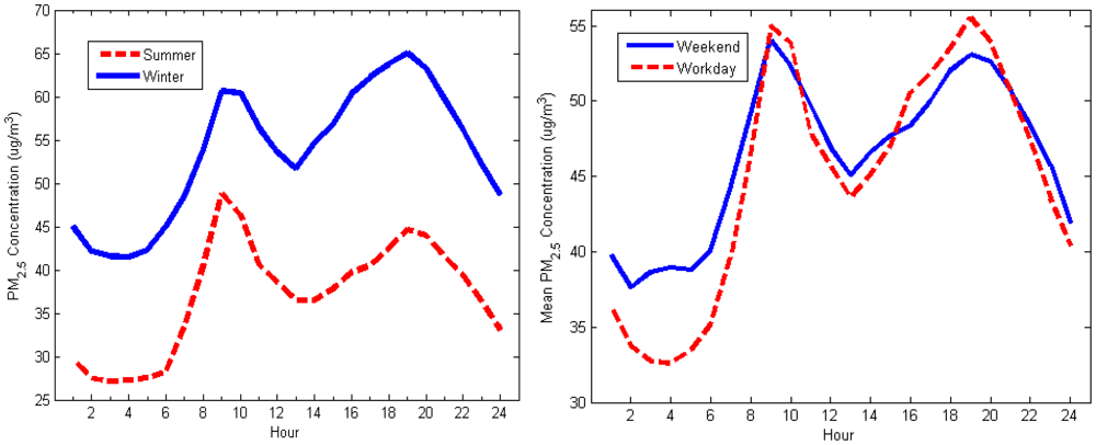
Despite a similar pattern observed in Figure 4 (left), summer diurnal PM2.5 concentrations is found to be lower than in winter. On the other hand, the peak values in Figure 4 (right) are higher on weekdays compared with weekends, which may be caused by more anthropogenic activities.
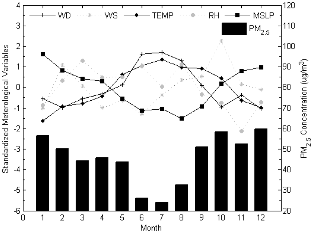
4.3. Monthly and Seasonal Trends of PM2.5 Concentration and Meteorological Data
Seasonal variations of PM2.5 were obvious (Figure 5). The concentrations are higher in winter and autumn and lower in spring and summer seasons. Previous studies of roadside suspended particulates at heavily trafficked urban areas in Hong Kong conducted in 2000 [37] and 2005 [40] showed similar seasonal patterns. The mean sea level pressure exhibits a similar pattern as PM2.5 characterized.
4.4. 3D PM2.5 Visualization and Query Prototype
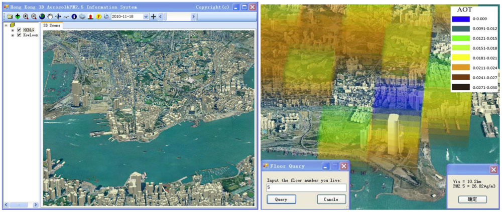
In order to understand the spatial pattern of PM2.5 concentrations in the context of the built-up environment of Hong Kong, a Geographic Information Systems (GIS) prototype was developed in this study to integrate atmospheric PM2.5 vertical profiles with 3D GIS data which are provided by the Hong Kong Lands Department. This prototype utilized ESRI ArcGIS Scene Control component to present the landscape objects including the terrain model, building polygons, AOTΔz and PM2.5Δz grid data in 3D space. The functionality of this system provides scene rendering using perspective view. The 3D PM2.5Δz atmospheric layers corresponding to 500 m pixel columns were rendered using a transparent color scheme overlaid with the 3D building polygons. Since the system is aimed at the built environment within the city, only seven PM2.5Δz atmospheric layers, each has 75 m elevation, were created. In this GIS prototype, each building is corresponding with its cadastral footprint polygon, which owns attributes including building height, number of floors and height of each floor (e.g., building height/number of floors). The PM2.5Δz data can be related with each building by tabular linkage through the polygon-in-polygon function of the Hawths extension [41]. Therefore, any floor of a building can be related to the PM2.5Δz concentrations and useful for direct query. The interface of this GIS prototype is shown in Figure 6 (left). Figure 6 (right) shows the query results of the PM2.5Δz concentrations of the International Commerce Centre on 1 February 2007 (local time 10:50).
5. Discussion and Conclusions
The paper presents a comprehensive study of characteristics, behavior and trends of PM2.5, as well as its correlation with different meteorological parameters and the state-of-the-art technique for modeling and visualizing of atmospheric PM2.5Δz vertical profiles. In this study, the hourly based dataset, e.g., PM2.5 concentrations and five meteorological parameters e.g., wind direction, wind speed, temperature, relative humidity, and pressure were analyzed to explore their diurnal and seasonal variations and interrelations.
PM2.5 showed a distinctive bimodal pattern with two marked peaks: morning rush hours (08:00–10:00) and evening rush hours (18:00–20:00), which are mostly influenced by the dense traffic. The lower PM2.5 concentrations observed in summer than in winter may be caused by the wind direction. Northerly and northeasterly winds bring pollutants from the Chinese mainland in winter, whereas southerly monsoon winds from the sea bring fresh air to the city in summer. In addition, the higher concentrations of PM2.5 in rush hours on weekdays compared to those in weekends suggest the significance of anthropogenic activities e.g., traffic-related local PM2.5 emissions.
The PM2.5Δz values for different atmospheric heights were linked to a GIS-based 3D urban model to provide near-real time visualization. The resulting 3D database of PM2.5Δz concentrations provides crucial information to air quality regulators and decision makers to comply with air quality standards and in devising control strategies. This prototype will be integrated with web-interface system in the near future.
Acknowledgments
This research was sponsored by the National Key Technology R&D Program of China (Grant No. 2012BAJ15B04) and the National High Technology Research and Development Program of China (Grant No. 2012AA12A305). The corresponding author was supported by the Young Thousand Talents Program of China (The Recruitment Program of Global Experts). The authors would like to thank the Hong Kong Observatory for the meteorological data, the Hong Kong Lands Department for GIS data, and Brent Holben of NASA for support of the Hong Kong AERONET stations.
References
- Dubovik, O.; Holben, B.; Eck, T.; Smirnov, A.; Kaufman, Y.; King, M.; Tanré, D.; Slutsker, I. Variability of absorption and optical properties of key aerosol types observed in worldwide locations. J. Atmos. Sci. 2002, 59, 590–608. [Google Scholar]
- Wallace, J.M.; Hobbs, P.V. Atmospheric Science, an Introductory Survey; Academic Press: New York, NY, USA, 1977; Volume 467. [Google Scholar]
- Hardin, M.; Kahn, R. Aerosols and Climate Change, 1999. Available online: http://earthobservatory.nasa.gov/Features/Aerosols/what_are_aerosols_1999.pdf (accessed on 8 May 2012).
- Kaufman, Y.J.; Tanré, D.; Gordon, H.R.; Nakajima, T.; Lenoble, J.; Frouin, R.; Grassl, H.; Herman, B.M.; King, M.D.; Teillet, P.M. Passive remote sensing of tropospheric aerosol and atmospheric correction for the aerosol effect. J. Geophys. Res. 1997, 102, 16815–16830. [Google Scholar]
- Liu, Y.; Paciorek, C.J.; Koutrakis, P. Estimating regional spatial and temporal variability of PM2.5 concentrations using satellite data, meteorology, and land use information. Environ. Health Perspect. 2009, 117, 886–892. [Google Scholar]
- Chan, L.Y.; Kwok, W.S. Vertical dispersion of suspended particulates in urban area of Hong Kong. Atmos. Environ. 2000, 34, 4403–4412. [Google Scholar]
- Cohen, A.J.; Anderson, H.R.; Ostro, B.; Pandey, K.D.; Krzyzanowski, M.; Künzli, N.; Gutyschmidt, K.; Pope, A.; Romieu, I.; Samet, J.M.; Smith, K. The global burden of disease due to outdoor air pollution. J. Toxicol. Environ. Health 2005, 68, 1301–1307. [Google Scholar]
- Ostro, B.; Feng, W.Y.; Broadwin, R.; Malig, B.; Green, S.; Lipsett, M. The impact of components of fine particulate matter on cardiovascular mortality in susceptible subpopulations. Occup. Environ. Med. 2008, 11, 750–756. [Google Scholar]
- Peng, R.D.; Chang, H.H.; Bell, M.L.; McDermott, A.; Zeger, S.L.; Samet, J.M.; Dominici, F. Coarse particulate matter air pollution and hospital admissions for cardiovascular and respiratory diseases among Medicare patients. J. Am. Med. Assoc. 2008, 299, 2172–2179. [Google Scholar]
- Arthur, T.D.; Owen, M.D. Temporal, spatial and meteorological variations in hourly PM2.5 concentration extremes in New York City. Atmos. Environ. 2003, 38, 1547–1558. [Google Scholar]
- Fraser, M.P.; Yue, Z.W.; Buzcu, B. Source apportionment of fine particulate matter in Houston, TX, using organic molecular markers. Atmos. Environ. 2003, 37, 2117–2123. [Google Scholar]
- Elminir, H.K. Dependence of urban air pollutants on meteorology. Sci. Total Environ. 2005, 350, 225–237. [Google Scholar]
- Dawson, J.P.; Adams, P.J.; Pandis, S.N. Sensitivity of PM2.5 to climate in the Eastern US: A modeling case study. Atmos. Chem. Phys. 2007, 7, 4295–4309. [Google Scholar]
- Jung, I.; Kumar, S.; Kuruvilla, J.; Crist, K. Impact of Meteorology on the Fine Particulate Matter Distribution in Central and Southeastern Ohio. Proceedings of the American Meteorological Society 12th Joint Conference on Applications of Air Pollution Meteorology with the Air and Waste Management Association Norfolk 2002, Boston, MA, USA, 20–24 May 2002.
- Hien, P.D.; Bac, V.T.; Tham, H.C.; Nhan, D.D.; Vinh, L.D. Influence of meteorological conditions on PM2.5 and PM2.5–10 concentrations during the Monsoon Season in Hanoi, Vietnam. Atmos. Environ. 2002, 36, 3473–3484. [Google Scholar]
- Chiang, P.; Chang, E.E.; Chang, T.; Chiang, H. Seasonal source-receptor relationships in a petrochemical industrial district over Northern Taiwan. J. Air Waste Manag. Assoc. 2005, 55, 326–341. [Google Scholar]
- Qin, Y.; Chan, C.K.; Chan, L.Y. Characteristics of chemical compositions of atmospheric aerosols in Hong Kong: Spatial and seasonal distributions. Sci. Total Environ. 1997, 206, 25–37. [Google Scholar]
- Louie, P.K.K.; Chow, J.C.; Chen, L.W.A.; Watson, J.G.; Leung, G.; Sin, D.W.M. PM2.5 chemical composition in Hong Kong: Urban and regional variations. Sci. Total Environ. 2004, 338, 267–281. [Google Scholar]
- So, K.L.; Guo, H.; Li, Y.S. Long-term variation of PM2.5 levels and composition at rural, urban, and roadside sites in Hong Kong: Increasing impact of regional air pollution. Atmos. Environ. 2007, 41, 9427–9434. [Google Scholar]
- Cheng, S.Q.; Lam, K.C. An analysis of winds affecting air pollution concentrations in Hong Kong. Atmos. Environ. 1998, 32, 2559–2567. [Google Scholar]
- Hong Kong Environmental Protection Department (HKEPD). Twelve-Month Particulate Matter Study in Hong Kong, Final Report 2002 Available online: http://www.epd.gov.hk/epd/english/environmentinhk/air/studyrpts/files/content.pdf (accessed on 8 May 2012).
- Levy, R.C.; Remer, L.A.; Mattoo, S.; Vermote, E.F.; Kaufman, Y.J. Second-generation operational algorithm: Retrieval of aerosol properties over land from inversion of Moderate Resolution Imaging Spectroradiometer spectral reflectance. J. Geophys. Res. 2007. [Google Scholar] [CrossRef]
- Wong, M.S.; Lee, K.H.; Nichol, J.E.; Li, Z.Q. Retrieval of aerosol optical thickness using MODIS 500 × 500 m2, a study in Hong Kong and Pearl River Delta region. IEEE Trans. Geosci. Remote Sens. 2010, 48, 3318–3327. [Google Scholar]
- Wong, M.S.; Nichol, J.E.; Lee, K.H. An operational MODIS aerosol retrieval algorithm at high spatial resolution, and its application over a complex urban region. Atmos. Res. 2011, 99, 570–589. [Google Scholar]
- Engel-Cox, J.A.; Hoff, R.M.; Haymet, A.D.J. Recommendations on the use of satellite remote-sensing data for urban air quality. J. Air Waste Manag. Assoc. 2004, 54, 1360–1371. [Google Scholar]
- Seinfeld, J.H.; Pandis, S.N. Atmospheric Chemistry and Physics: From Air Pollution to Global Change; John Wiley & Sons: New York, NY, USA, 1998. [Google Scholar]
- Wang, J.; Christopher, S.A. Intercomparison between satellite derived aerosol optical thickness and PM2.5 mass: Implications for air quality studies. Geophys. Res. Lett. 2003, 30. [Google Scholar] [CrossRef]
- Wong, M.S.; Nichol, J.E.; Lee, K.H.; Lee, B.Y. Monitoring particulate matter 2.5 μm within urbanised regions using satellite-derived aerosol optical thickness, a study in Hong Kong. Int. J. Remote Sens. 2011, 32, 8449–8462. [Google Scholar]
- Wong, M.S.; Nichol, J.E.; Lee, K.H. Modeling of aerosol vertical profiles using GIS and remote sensing. Sensors 2009, 9, 4380–4389. [Google Scholar]
- Nichol, J.E.; Wong, M.S.; Wang, J.Z. A 3D aerosol and visibility information system for urban areas using remote sensing and GIS. Atmos. Environ. 2010, 44, 2501–2506. [Google Scholar]
- Yasuhiro, S. Tropospheric aerosol extinction coefficient profiles derived from scanning lidar measurements over Tsukuba, Japan, from 1990 to 1993. Appl. Opt. 1996, 35, 4941–4952. [Google Scholar]
- Elterman, L. Relationships between vertical attenuation and surface meteorological range. Appl. Opt. 1970, 9, 1804–1810. [Google Scholar]
- Qiu, J.; Zong, X.M.; Zhang, X.Y. A study of the scaling height of the tropospheric aerosol and its extinction coefficient profile. J. Aerosol Sci. 2005, 36, 361–371. [Google Scholar]
- Koschmieder, H. Theorie der horizontalen Sichtweite, Beiträge zur Physik der freien Atmosphäre. Meteorol. Z. 1924, 12, 33–53. [Google Scholar]
- Hanel, G. The properties of atmospheric aerosol particles as function of the relative humidity at thermodynamic equilibrium with the surrounding atmosphere. Adv. Geophys. 1976, 19, 73–188. [Google Scholar]
- Fitzgerald, J.W.; Hoppel, W.A.; Vietti, M.A. The size and scattering coefficient of urban aerosol particles at Washington, DC as a function of relative humidity. J. Atmos. Sci. 1982, 39, 1838–1852. [Google Scholar]
- Chan, L.Y.; Kwok, W.S. Roadside suspended particulates at heavily trafficked urban sites of Hong Kong—Seasonal variation and dependence on meteorological conditions. Atmos. Environ. 2001, 35, 3177–3182. [Google Scholar]
- Pankow, J.F.; Storey, J.M.E.; Yamasaki, H. Effect of relative humidity on gas/particle partitioning of semivolatile organic compounds to urban particulate matter. Environ. Sci. Technol. 1993, 27, 2220–2226. [Google Scholar]
- Zhan, X.J.; Zhang, X.L.; Xu, X.F.; Xu, J.; Meng, W.; Pu, W.W. Seasonal and diurnal variations of ambient PM2.5 concentration in urban and rural environments in Beijing. Atmos. Environ. 2009, 43, 2893–2900. [Google Scholar]
- Cheng, Y.; Ho, K.F.; Lee, S.C.; Law, S.W. Seasonal and diurnal variations of PM1.0, PM2.5 and PM10 in the roadside environment of Hong Kong. China Particuol. 2006, 4, 312–315. [Google Scholar]
- Beyer, H.L. Hawth's Analysis Tools for ArcGIS 2004. Available online: http://www.spatialecology.com/htools (accessed on 8 May 2012).


| Correlation (r) | PM2.5 | WD | WS | TEMP | RH | MSLP |
|---|---|---|---|---|---|---|
| PM2.5 | 1.000 | −0.101 | 0.095 | −0.478 | −0.366 | 0.504 |
| WD | −0.101 | 1.000 | −0.683 | 0.291 | −0.052 | −0.342 |
| WS | 0.095 | −0.683 | 1.000 | −0.220 | 0.011 | 0.222 |
| TEMP | −0.478 | 0.291 | −0.220 | 1.000 | 0.083 | −0.866 |
| RH | −0.366 | −0.052 | 0.011 | 0.083 | 1.000 | −0.338 |
| MSLP | 0.504 | −0.342 | 0.222 | −0.866 | −0.338 | 1.000 |
© 2012 by the authors; licensee MDPI, Basel, Switzerland This article is an open access article distributed under the terms and conditions of the Creative Commons Attribution license (http://creativecommons.org/licenses/by/3.0/).
Share and Cite
Shi, W.; Wong, M.S.; Wang, J.; Zhao, Y. Analysis of Airborne Particulate Matter (PM2.5) over Hong Kong Using Remote Sensing and GIS. Sensors 2012, 12, 6825-6836. https://doi.org/10.3390/s120606825
Shi W, Wong MS, Wang J, Zhao Y. Analysis of Airborne Particulate Matter (PM2.5) over Hong Kong Using Remote Sensing and GIS. Sensors. 2012; 12(6):6825-6836. https://doi.org/10.3390/s120606825
Chicago/Turabian StyleShi, Wenzhong, Man Sing Wong, Jingzhi Wang, and Yuanling Zhao. 2012. "Analysis of Airborne Particulate Matter (PM2.5) over Hong Kong Using Remote Sensing and GIS" Sensors 12, no. 6: 6825-6836. https://doi.org/10.3390/s120606825