Simultaneous Source Localization and Polarization Estimation via Non-Orthogonal Joint Diagonalization with Vector-Sensors


Abstract
: Joint estimation of direction-of-arrival (DOA) and polarization with electromagnetic vector-sensors (EMVS) is considered in the framework of complex-valued non-orthogonal joint diagonalization (CNJD). Two new CNJD algorithms are presented, which propose to tackle the high dimensional optimization problem in CNJD via a sequence of simple sub-optimization problems, by using LU or LQ decompositions of the target matrices as well as the Jacobi-type scheme. Furthermore, based on the above CNJD algorithms we present a novel strategy to exploit the multi-dimensional structure present in the second-order statistics of EMVS outputs for simultaneous DOA and polarization estimation. Simulations are provided to compare the proposed strategy with existing tensorial or joint diagonalization based methods.1. Introduction
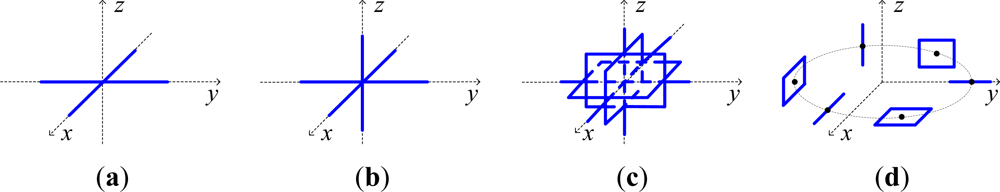
An electromagnetic vector-sensor (EMVS) comprises 2∼6 electromagnetic (EM) sensors (e.g., orthogonally oriented short dipoles and small loops arranged in a co-located or distributed manner, see Figure 1) that provide complete or partial measurements of the EM fields induced by the incident sources [1–5]. As a result, using EMVS in direction finding and polarization estimation could yield additional advantages over the conventional scalar sensor array processing techniques, mainly due to the fact that the distinction of impinging sources could be well exploited in both the spatial and polarization domains by using EMVS arrays. Particularly, in the early works on direction finding and polarization estimation with EMVS’s, maximum likelihood (ML) [3,6,7], multiple signal classification (MUSIC) [8–10], subspace fitting [11,12], and estimation of signal parameters via rotational invariance techniques (ESPRIT) [13–18] have been derived from their scalar array based counterparts, and some other issues such as vector cross-product based source tracking [4,19,20], polarimetric smoothing for coherent source localization [21–24], the analysis of performance [25,26] and identifiability [27–31] were also addressed.
The early works unfolded the potential of using EMVS’s in array processing through both analysis and experiments. However, there was still a problem as these works rarely considered the multi-dimensional (MD) data structure of the EMVS array outputs in the time-space-polarization domains. More exactly, the ML and MUSIC variants usually concatenate the vectorial output from each EMVS into a long-vector, which somehow undermines the MD structure of the array outputs. The ESPRIT variants, on the other hand, did consider this MD structure of array outputs in the form of multiple rotational invariant matrix slices, yet only used these matrix slices in a pairwise manner such that only a fraction of the MD structure is exploited each time. As such, the use of higher-dimensional algebras such as tensors and hypercomplex has attracted increasing attention in the recent years [32–44], for a better exploitation of the afore-mentioned MD structure present in the EMVS signals. More exactly, tensors are employed to model the MD structure of EMVS array signals as a multilinear algebraic quantity, upon which parallel factor analysis (PARAFAC) and higher-order singular value decomposition (HOSVD) are used to exploit this presented multilinearity [32–37]. Hypercomplexes, on the other hand, handled the above-mentioned MD structure by encapsulating the local vectorial output of each EMVS into a multinion (e.g., quaternion, biquaternion, quad-quaternion, bicomplex, or a more generalized geometric algebra model) [38–43], of which multiple imaginary parts are used and defined under certain hypercomplex algebraic rules. Recently, there have also been works on combining tensor decompositions and hypercomplex operations [44]. It is demonstrated in these works that an efficient exploitation of the MD structure for EMVS array signals could bring out improved performance over the conventional methods, with regards to the robustness to the errors introduced by noise, finite data length, and model errors.
In this paper, we will introduce an alternative strategy to tensor and hypercomplex based methods, for exploiting the MD structure of the outputs for an array of six-component cocentered complete EMVS’s (for clarity hereafter we name it EMVS without causing any misunderstanding), in the context of joint DOA and polarization estimation. More specifically, we formulize the MD structure of an EMVS array outputs as a set of complex square matrices that share a jointly diagonalizable structure, and propose to fit this structure by complex-valued non-orthogonal joint diagonalization (CNJD) for simultaneous DOA and polarization estimation. Moreover, we consider the LU or LQ decompositions for the target matrices and formulize the optimization problem in CNJD as two alternating stages: the L-stage and U(Q)-stage. In addition, inspired by the Jacobi-type schemes for joint diagonalization, we further replace the sub-optimization problem in each of the above two stages by a sequence of elementary rotation matrices which rely on only one or two parameters, and propose two closed-form CNJD algorithms.
The rest of the paper is organized as follows: Section 2 presents the data model of an EMVS array, and its formulation into CNJD problems. Section 3 introduces three proposed CNJD algorithms and the corresponding joint DOA and polarization estimation strategy, as well as some implementation remarks. Section 4 provides simulations to compare the proposed strategy with some existing tensorial methods to illustrate the potential of the proposal. Section 5 concludes the manuscript.
2. Measurement Model and Problem Formulation
2.1. Measurement Model of an EMVS Array Output
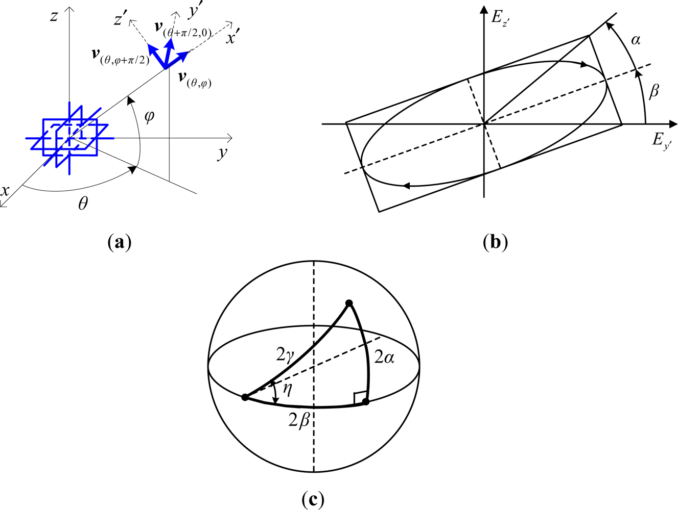
Let (θ,φ) be the azimuth-elevation 2D DOA of a narrow-band planar EM signal (see Figure 2(a) for the angle definition). The induced electric field vector of this signal moves along the polarization ellipse which could be characterized by the ellipse angle α and orientation angle β, and the polarization state could further be represented by (γ,η) that are linked to (α,β) in the Poincare sphere [1] (see Figure 2(b,c) to visualize the polarization ellipse and the relationship between(γ,η) and (α,β)), 0 < θ < 2π, |φ| ≤ π/2, 0 < γ < π/2, |η| ≤ π. The output of an EMVS is written as [2]:
In addition to the unit-EMVS formulization in Equation (1), we further assume the receiving antenna array comprises N EMVS’s. The position coordinates of the nth EMVS are encapsulated in a vector kn ∈ R3, n =1, 2, …, N. As a result, the phase delays of all the EMVS’s with regards to the one at the origin could be characterized by the so-called spatial steering vector defined as follows:
In the presence of M impinging signals and additive noise, the EMVS array output is given by:
In addition, we herein give the following assumptions:
The sources are zero-mean, stationary, and mutually uncorrelated;
The noises are zero-mean, stationary, and uncorrelated with the sources.
The sources have distinct DOA’s, and any arbitrary K (K ≤ N) spatial steering vectors associated with different DOA’s are linearly independent.
Next, we shall show how to formulize the second-order statistics of the EMVS array output given in Equation (4) into a set of jointly diagonalizable square matrices.
2.2. Formulation of the Second-Order Statistics into Jointly Diagonalizable Matrices
We denote the outputs of the nth EMVS’s as xn(t) ∈ C6. By definition, we know that xn(t) is the nth column of X(t) and thus could be further formulized as , where dm,n is the nth element of dm, and nn(t) ∈ C6 is the noise term on this EMVS. As a result, performing cross covariance between xl(t) and xk(t) under assumptions 1 and 2 yields (l, k =1, 2, …, N):
Remark 1: It is important to note that the target matrix P is complex-valued and non-orthogonal as in most of the cases. Moreover, Cl,k is non-Hermitian for l ≠ k. As a result, it is preferable to use complex non-orthogonl joint diagonalization (CNJD) methods for non-Hermitian matrices, for the identification of P.
Remark 2: We note that most of the joint diagonalization algorithms assume that the target matrix be square, while in our problem P is mostly not square. As a result, we modify Equation (5) a little bit as follows (here we assume M ≤ 6):
3. Proposed Algorithm
As indicated in Section 2, the EMVS array signals could be formulated in a set of complex non-orthogonal jointly diagonalizable matrices in the domain of second-order statistics, and the problem of joint DOA and polarization estimation might be solved by identifying this structure via CNJD algorithms. In this section, we firstly propose two CNJD algorithms using the Jacobi-type scheme and LU/LQ decompositions. Then we propose a novel strategy for simultaneous direction finding and polarization estimation based the proposed CNJD algorithms, as well as some discussion.
3.1. Complex Non-Orthogonal Joint Diagonalization via Jacobi-Type Scheme and LU/LQ Decompositions
We assume a set of complex matrices C = {C1, …, CK} share the jointly diagonalizable structure as given in Equation (6): Ck = ADkAH. Here we neglect the noise term and combine the two indices (l,k) for Cl,k and Dl,k in Equation (6) as one index k for clarity. Moreover, we consider the general case that {C1, …, CK} are of size L × L for the proposed CNJD algorithms (in our particular case of joint DOA and polarization estimation with EMVS’s, L is equal to 6 according to Equation (6)). The goal of joint diagonalization is to seek an estimate for B ≜ A−1 such that {BCkBH} are as diagonal as possible. To solve this problem, we consider the following criterion for the estimation of B:
Moreover, we adopt the Jacobi-type scheme to solve Equations (9a) and (9b) via a set of rotations which are repeated sequentially for all the possible index pairs (i, j) as follows, 1 ≤ i < j ≤ L:
Firstly, we consider the LU decomposition based algorithm. In this case, the matrix V in Equation (9a) is an upper-triangular matrix U ∈ CL×L, and T(i,j) in Equation (10b) is an elementary upper-triangular matrix which is equal to the identity matrix except the (i, j)th upper entry αi,j, 1 ≤ i < j ≤ L. In addition, for index pair (i, j), we note that only impacts the ith row and column of Ck,old, k = 1, …, K, and thus the minimization of amounts to minimizing the sum-of squared norms of the off-diagonal elements in the ith row and column of Ck,new:
We note that Ck,new (i, p) = αi,j Ck,old (j, p) + Ck,old (i, p) and . As a result, substituting these formulations into Equation (11) yields the following equation after a few simple manipulations:
Setting the derivative of ξi,j with regards to yields the optimal estimate of αi,j as:
As for the L-stage, we note herein that the only difference is the use of lower-triangular matrix instead of the upper-triangular one in the U-stage. Therefore, Equation (13) is still valid for the optimal estimate of the factor involved in the L-stage, except that the indices i and j are transposed.
In the second algorithm, we consider the LQ decomposition of B, and thus the matrix V in Equation (9a) is a unitary matrix Q ∈ CL×L. Hence, the sub-optimization problem in the Q-stage as indicated in Equation (9a) is indeed an orthogonal joint diagonalization (OJD) problem which could be solved by Cardoso’s Jacobi-type algorithm [45]. As such, in the second algorithm we use Cardoso’s OJD algorithm in the Q-stage, followed by the L-stage which is addressed in the first proposed algorithm.
Now that we have obtained the L-stage and U(Q)-stage for the proposed algorithms, we loop these two stages until convergence is reached. In addition, we note that there would be several ways to monitor the convergence for the proposed CNJD algorithms. For example, we could terminate the iterations when the parameter values in each iteration of the L-stage or U(Q)-stage are small enough, which indicate a minute contribution from the elementary rotations, and hence convergence. We might as well monitor the sum of off-diagonal squared norms in each iteration, and terminate the loops when the change in it is smaller than a preset threshold. In the following context of our manuscript, we adopt a third way which stops the iterations when the values of between two successive complete runs of L-stage and U(Q)-stage are close enough, with regards to a preset threshold τ, where I denotes the identity matrix. We name the proposed LU and LQ based algorithms as LUCJD and LQCJD, respectively, and summarize them in Table 1.
3.2. Joint DOA and Polarization Estimation with CNJD
Given the proposed LUCJD and LQCJD algorithms, we could identify the jointly diagonalizable structure of an EMVS array outputs as given in Equation (6), for the estimation of A = B−1. Moreover, we note that the identification of A implies estimates of the angular-polarization steering vectors pm, which could be used to estimate the source DOA’s and polarizations. In addition, it is important to note that the target matrices as given in Equation (5) are all of dimensionality 6 × 6, and therefore the sensitivity issue for non-orthogonal JD with very few large matrices would not occur in our applications.
However, it is important to note that A is required to be square for the proposed CNJD algorithms, and thus the estimation of A by using these algorithms does not only contain the desired estimates of pm, but also the contribution from the noise, as is formulated in Equation (6) (we denote the estimates of A, B, and pm by Ã, B̃, and p̃m, respectively, m =1, 2, …, M). Therefore, before performing joint DOA and polarization estimation, we need to firstly separate the columns of à associated with the sources from those contributed by noise. This procedure is similar to signal/noise subspace estimation which is key to subspace based methods such as MUSIC and ESPRIT. However, noting that à is not constrained to be orthogonal, we could not separate its columns into the signal and noise subspaces by simply selecting the columns corresponding to the largest M diagonal elements of {B̃Cl,k B̃H}, as is done for MUSIC and ESPRIT. As such, we propose the following scheme to solve this problem.
Firstly, we stack all the matrices Cl,k as given in Equation (5) into a big matrix C ∈ C36×N2 as :
Secondly, we note that B̃Cl,k B̃H is actually an estimate of Dl,k in Equation (6), and where Ξ ∈ CM×M is a diagonal matrix with the mth diagonal element equal to , according to Equations (5) and (6), l,k = 1, …, N. As a result, we have:
Finaly, we use the indices obtained above to select the columns of à that correspond to the estimates of the angular-polarization steering vectors p̃m = Ã(;,λm).
With the obtained estimates {p̃m | m = 1,2,...,M}, and denoting , where ẽm, h̃m ∈ C3, we adopt the scheme in [13,14] to calculate the DOA and polarization estimates as follows:
We summarize the proposed joint DOA and polarization estimation strategy in Table 2.
3.3. Discussion
In this subsection we present some remarks to provide insights into the proposed CNJD algorithms and the joint DOA and polarization estimator:
Remark 3 (Concerning the adopted CNJD algorithms): Besides the proposed LUCJD and LQCJD methods, we could also use other joint diagonalization algorithms for the considered problem of simultaneous DOA and polarization estimation. We herein note that our proposed algorithms are of nice flexibility in various applications, as they assume neither Hermitianity nor positive definiteness on the matrices, which are often imposed by other CNJD algorithms [46,47,57]. In addition, compared with CNJD methods based on gradient or Newton-type optimization [51,52], the proposed algorithms are of closed-form in each iteration, and do not involve issues such as learning rate adjustment. Furthermore, we note that our algorithms could be considered as a generalization of the works in [53–55], which considered parametrized Jacobi-type non-orthogonal joint diagonalization for real-valued matrices. In particular, the work in [53] firstly considered non-orthogonal Jacobi-like algorithms based on LU and LQ decompositions, and was extended to the complex domain in [57]. However, we note that the algorithm in [57] considered only Hermitian matrices, and is thus essentially distinct from our proposed algorithms. There are also some other Jacobi-like algorithms, most of which consider only the real-valued cases [53–56]. Recently, there have been works devoting to Jacobi-like complex non-orthogonal CNJD algorithms [50,57].
Remark 4(On the link to tensorial methods): It should be noted that our problem could also be tackled by tensorial methods. In particular, stacking the matrices {Cl,k | l,k = 1, …, N} given in Equation (5) along a third dimension would yield a trilinear tensor [35,36], and these matrices could also be arranged into a quadralinear tensor according to [37]. Therefore, the joint estimates for DOA and polarization could be obtained by performing parallel factor analysis (PARAFAC) upon these tensor models. Compared with these tensorial methods, we note that the CNJD mostly considered the ‘square’ case as indicated in Remark 2 while PARAFAC could handle the non-square case. As a result, the CNJD based strategy is usually combined with subspace methods to select the desired columns from the square estimates.
Another noteworthy property of CNJD based strategies is that CNJD is usually very robust to noise with structured covariance, which would yield additional contribution to the joint diagonalizable structures other than sources. Therefore, the proposed CNJD based strategy might be robust to colored noise or interferences. On the other hand, the mostly used alternating least squares (ALS) methods for the implementation of PARAFAC are sometimes sensitive to erroneous prediction of the underlying parallel factors (e.g., underfactoring) [58], such that the presence of coherent noise with structured covariance would deteriorate the performance of PARAFAC based strategies, even if the number of sources is correctly predicted. However, in contrary to the above nice property, the CNJD algorithms are sensitive to unstructured noise such as white noise. In practice, we note that the array noise is usually spatially colored with the covariance between different elements admitting some particular structure [44], and therefore the CNJD based strategy would be well adapted to practical scenarioes.
Remark 5(On the independence of knowledge on spatial configuration): A main property of the proposed method is that the joint estimation for DOA and polarization mainly relies on the estimates of angular-polarization steering vectors, while the estimates of spatial steering vectors that are indicated in the diagonal elements of {B̃Cl,kB̃H} are only used in the noise subspace projection stage to select the desired columns of the estimate Ã. As such, the proposed approach does not require any knowledge on the spatial configuration of the array, and is therefore of much flexibility in applications where precise knowledge on the position of each EMVS is unavailable. Meanwhile, the above independence of the spatial prior knowledge for the proposed strategy would lead to another advantage, that the adopted array might be spatially sparse, which enables enlarged spatial aperture.
Remark 6(On the identifiability): An issue of great interests is the identifiability property of the proposed strategy and this issue comprises two aspects, that are: (1) the least number of EMVS’s that are required for a successful implementation of the proposed method; and (2) the most number of sources that could be uniquely identified. To address the former, we note that the jointly diagonalizable structure could be uniquely identified for at least two matrices, and hence we need at least two EMVS’s for the proposed method (a simple example is the ESPRIT algorithm). For the latter issue, we simply notice that the number of sources could not exceed six to meet the “square” requirement of the proposed LUCJD and LQCJD algorithms. We note herein that the above analysis is given under assumption A3) in Section II, which excludes the scenarioes that two or more target matrices for CNJD are proportional or linearly dependent. A more challenging problem is the identification of several sources with identical DOA, and this requires a thorough analysis of the identifiability for CNJD. However, this issue is beyond the scope of this manuscript and will be the focus of our future work.
Remark 7(On the computational complexity): Another important issue about the proposed LUCJD and LQCJD is the computational complexity, and this issue comprises two aspects, that are: (1) The computational complexity for one sweep; and (2) the number of sweeps until convengence. For the former, we note that one sweep in these algorithms comprises two stages, each of which undergoes L(L – 1)/2 elementary rotations (L is the dimensionality of the target matrices). Moreover, we note that the update of target matrices involve 2L2 complex multiplication operations and the update of matrices L or U (Q) involve L2 complex multiplications according to Equation (10). The calculation of the optimal αi, j involves 4K(L – 1) multiplications (there is also a division, ignored as it contributes little to the complexity) according to Equation (3). The Q-stage in LQCJD involves 9K multiplications and an eigendecomposition of a 3 × 3 matrix. Therefore, the computational loads of one sweep of LUCJD and LQJCD are 3L3(L – 1) + 4KL(L – 1)2, and 3L3(L – 1) + 2KL(L – 1)2 + (9K + ξ)L(L – 1)/2, respectively, where ξ is the complexity of computing the eigendecomposition of a 3 × 3 matrix. We note herein that the computational complexity of LUCJD and LQCJD per sweep is approximately larger than that of other Jacobi-type algorithms (e.g., JTJD [50]) as each sweep of LUCJD and LQCJD incorporates two stages while other methods only have one stage in each sweep.
As for the number of sweeps that LUCJD and LQCJD take until convergence, we note that LQCJD converges nearly quadratically, mainly because the algorithm in the Q-stage is of quadratic converging pattern. The converging pattern of LUCJD, however, is linear as inherited from its real counterpart [53].
4. Simulation Results
In this section, we present simulations to verify the proposed joint DOA and polarization estimation strategy, and compare it with other methods of similar type (e.g., tensorial algorithms). The impinging signals are assumed to be far-field narrow-band signals of equal carrying frequency, and the adopted array is a sparse linear array with interspacing identical to twice the wavelength (the number of sources and EMVS’s are set differently in various simulations). In addition, the noise is formulated following the reports on sensor array noise modeling [44] as:
We use the Overall Root Mean Squared Angular Error (RMSAE) [2] to measure the accuracy of DOA estimates as , where vθm,φm and vθ̃m,φ̃m are the mth true and estimated poynting vectors, respectively. In addition, we use the Overall Mean Squared Errors (RMSE) to measure the estimation accuracy of the two polarization parameters. Furthermore, SNR used in all the simulations is defined as SNR ≜ 10log10 (ps / pε), where ps and pε are the signal power and noise power per vector-sensor, respectively. In the following, the first simulation is performed to verify our identification analysis in Remark 6, Section 3. In the second simulation, the proposed strategy is compared with other methods of similar type, with regards to the robustness to different errors (e.g., the errors caused by noise, finite data length, and noise covariance). The third simulation concerns the converging pattern of the proposed LUCJD and LQCJD algorithms.
4.1. Simulation for Six Sources Incident on Two EMVS’s
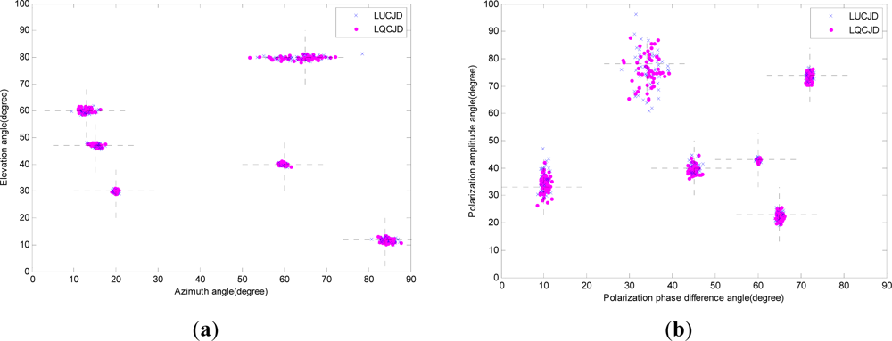
In the first simulation, we consider the scenario that six sources are impinging on an array of two EMVS’s, to verify our identification analysis in Remark 6, Section 3. We note that in this case the number of sources reaches the upper-bound, while the EMVS number reaches the lower-bound according to Remark 6, and thus this is the most difficult case to the identifiability for the proposed strategy. The source DOA’s are (θ1, φ1) = (47°, 15°), (θ2, φ2) = (12°, 84°), (θ3, φ3) = (40°, 60°), (θ4, φ4) = (30°, 20°), (θ5, φ5) = (60°, 13°), and (θ6, φ6) = (80°, 65°). The source polarizations are (γ1, η1) = (72°, 74°), (γ2, η2) = (60°, 43°), (γ3, η3) = (10°, 33°), (γ4, η4) = (65°, 23°), (γ5, η5) = (45°, 40°), and (γ6, η6) = (34°, 78°). In addition, we fix the SNR to 30 dB, fix the number of snapshots to 1000, set the noise covariance levels in Equations (18a)∼(18c) as (ρ1, ρ2) = (0.5, 0.5), and perform 50 independent runs for both LUCJD and LQCJD based algorithms. We here note that SNR in this scenario is set to a high level so that the impact of noise on the result could be ignored, and thus enabling a clearer illustration of the identifiability property of the proposed strategy. The distributions of DOA and polarization estimates are plotted in Figure 3. We note from the figure that the results from 50 independent runs assemble around the true values of the source DOA’s and polarizations denoted by crossed dashed lines, and this verifies our identifiability analysis in Remark 6 that our proposed strategy could successfully identify at most six sources with at least two EMVS’s.
4.2. Comparison with Other CNJD and PARAFAC Based Algorithms
In the second simulation, we compare the proposed methods with the trilinear PARAFAC based algorithm, a natural competitor to the proposed algorithms, noting that they have similar features with regards of the modeling and processing of the trilinear MD structure, such that the pros and cons of both methods could be fairly illustrated. The quadrilinear PARAFAC, however, is not included in the comparison, as it exploits fourth-order multilinearity of the present data statistics, and thus is not a natural competitor to CNJD and trilinear PARAFAC which concern third-order multilinearity. In addition, it is also of great interests to see how the proposed strategy would perform if the CNJD stage is carried out with other algorithms instead of the proposed LUCJD and LQCJD. Hence, we shall also include in the comparisons some other CNJD methods such as the nonparametric Jacobi transformation based joint diagonalization (JTJD) [50], the fast approximate joint diagonalization (FAJD) [48], and the uniformly weighted exhausive diagonalization by Gaussian iteration (UWEDGE) [49]. We select these methods mainly due to their similar nature to the proposed LUCJD and LQCJD algorithms (complex, non-orthogonal, and do not require Hermianity nor non-negative definiteness). In addition, the PARAFAC based method in our comparison uses the trilinear PARAFAC model in the subspace domain, as introduced in [32], and adopts the joint diagonalization strategy [59] along with compression based factor analysis [60] algorithm (COMFAC) to accelerate the trilinear decomposition. For the compared CNJD algorithms, LUCJD, LQCJD, and JTJD are initialized with identity matrix, while FAJD and UWEDGE adopt the coarse outputs of the orthogonal joint diagonalization as the initialization. The reason for the above different initializations is that these CNJD algorithms are of two different types (LUCJD, LQCJD, and JTJD are Jacobi-like, and FAJD, UWEDGE are with the weighted least squares criterion), and we strive to make the comparisons fair by letting these algorithms operate with their standard settings.
We consider the scenario that three sources are impinging upon an array of six EMVS’s. The array configuration is given at the begining of Section 4. The source DOA’s are (θ1, φ1) = (47°, 15°), (θ2, φ2) = (12°, 84°), and (θ3, φ3) = (40°, 60°). The source polarizations are (γ1, η1) = (72°, 74°), (γ2, η2) = (60°, 43°), and (γ3, η3) = (10°, 33°).
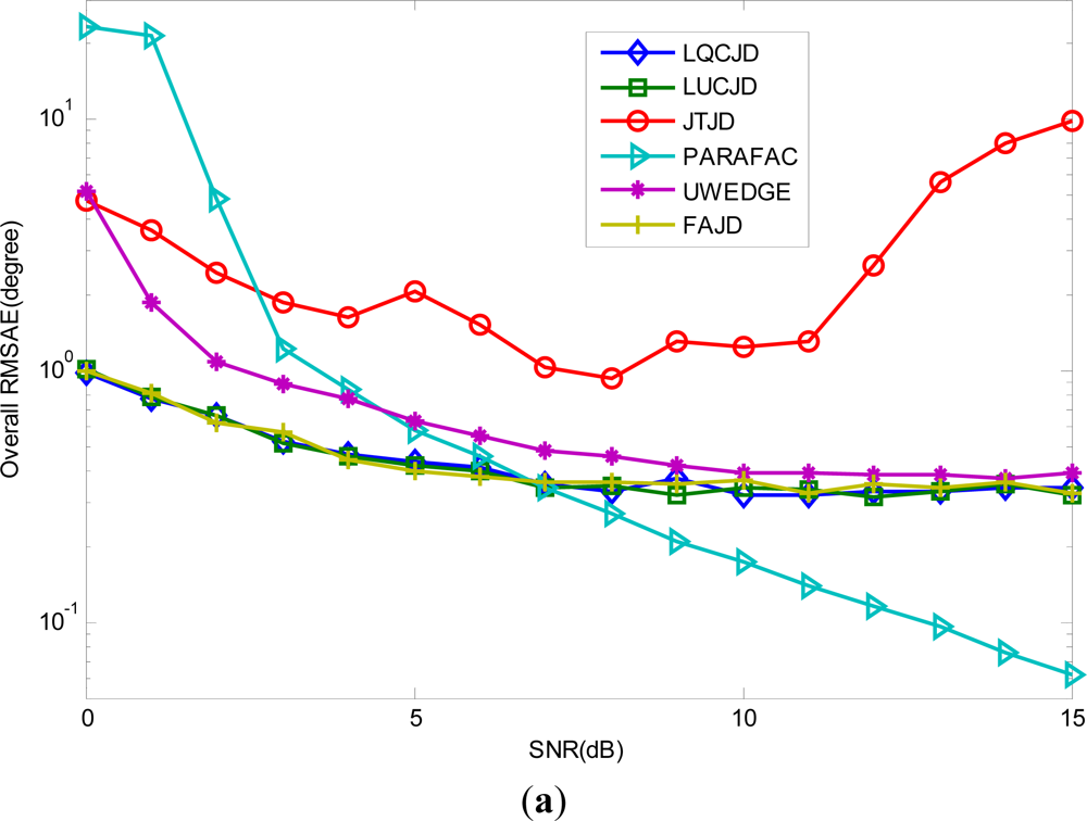
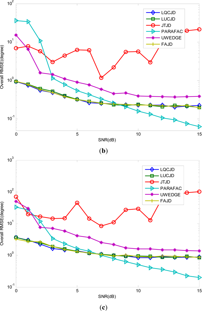
Firstly, we set the noise covariance levels (ρ1, ρ2) = (0.8, 0.8), set the number of snapshots to 1,000, and let SNR vary between 0 dB∼15 dB. The results obtained from 100 independent runs are plotted in Figure 4. We observe from the results that the proposed LUCJD and LQCJD algorithms provide almost equal precision as well as FAJD, and UWEDGE slightly underperforms these three algorithms. Furthermore, we note that the curves of LUCJD, LQCJD, FAJD, and UWEDGE drop more smoothly than PARAFAC, which indicates an improved robustness to colored noise of CNJD based methods over the PARAFAC based one. In particular, the proposed LUCJD and LQCJD outperform PARAFAC for low SNR levels (0∼6 dB), while PARAFAC performs better for high SNR levels (7∼15 dB). In addition, we note that JTJD underperforms the other algorithms with regards to the overall accuracy of DOA and polarization estimates. The main reason is that JTJD behaves unsteadily in our simulations, and sometimes converges to false solutions (we could draw the distribution of DOA and polarization estimates similarly to Figure 3 for JTJD to clearly show that it converges to false solutions for quite a few independent runs). We also note that UWEDGE slightly underperforms FAJD, LUCJD, and LQCJD with regards to the estimation accuracy. This is mainly because the WLS criterion based algorithms usually perform better with a set of properly designed weights for target matrices while UWEDGE adopts identical ones only.
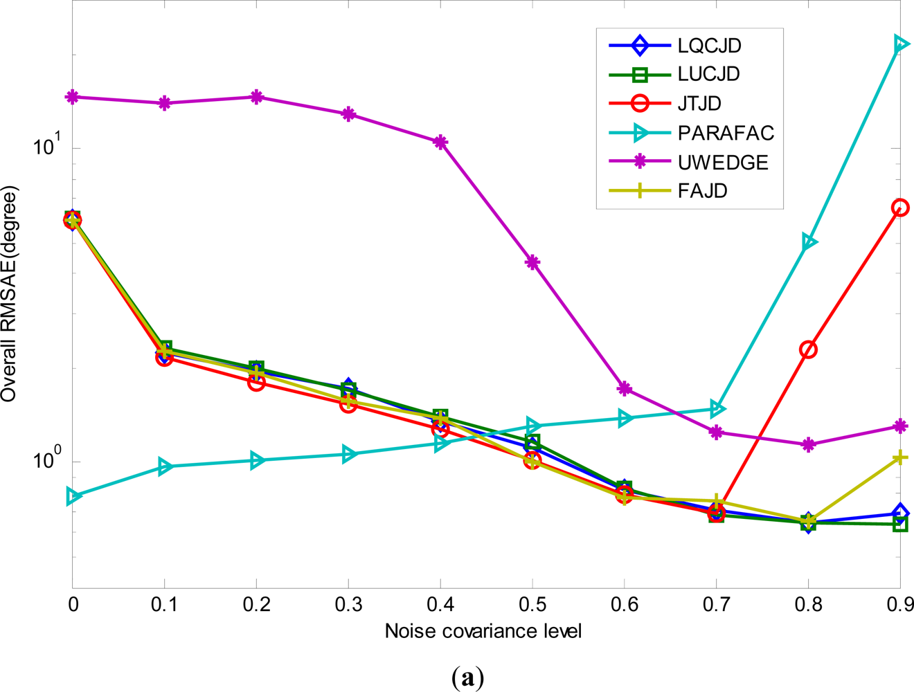
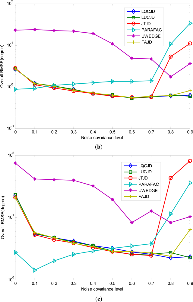
Secondly, we fix SNR and the number of snapshots to 2 dB and 1,000, respectively, and let the noise covariance levels ρ1 = ρ2 vary from 0∼0.9. The results from 100 independent runs are demonstrated in Figure 5. We can see quite diverse behaviors for CNJD and PARAFAC based strategies with the noise covariance changing, which clearly demonstrate the pros and cons of both strategies. More exactly, we note that the increase in noise covariance would generally improve the performance of CNJD based methods. In particular, the proposed LUCJD and LQCJD provide the best performance among all the CNJD algorithms with regards to the accuracy of joint DOA and polarization estimation. In addition, FAJD and JTJD provide almost equal performance as LUCJD and LQCJD for low noise covariance levels, yet become unsteady for ρ1 = ρ2 ≥ 0.8 and ρ1 = ρ2 ≥ 0.9, respectively. This is because the CNJD methods, especially the proposed LUCJD and LQCJD, are usually very robust to noise with structured covariance, which would yield additional contribution to the joint diagonalizable structures other than sources. Moreover, we note that PARAFAC, on the other hand, behaves inversely to the CNJD ones, as the increase in noise covariance results in a dramatic rise in the its curves. This is because the PARAFAC algorithms are usually sensitive to underfactoring (the number of parallel factors in the tensor model is greater than the number of sources) [58] and noise with high covariance levels would result in such underfactoring (when noise covariance increases, noise becomes interference, and thus contributes an additional factor to the PARAFAC model). The above observations are in accordance with our analysis in Remark 4, Section 3, that CNJD performs better than PARAFAC with regards to the robustness to color noise, yet the latter has stronger ability in suppressing white noise.
4.3. Comparison on the Convergence of CNJD Algorithms
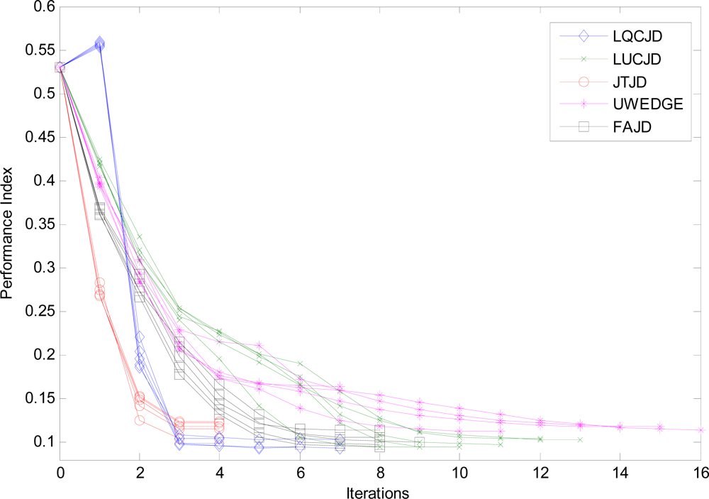
In the third simulation, we examine the converging properties of all the compared CNJD algorithms via an iteration-by-iteration evaluation by the use of performance index (PI) [54] which is defined as:
In addition, we terminate the iterations for all the CNJD algorithms when the decrease in PI values for two successive iterations (normalized by the current PI value) is smaller than 10−2. We note that it is impossible to monitor the values of PI as is done in this simulation in practice, as the knowledge of A is generally unavailable. The reasons for us doing so are: (1) to emphasize the converging patterns of the compared algorithms which are best illustrated by PI values for all the undergone iterations; and (2) to enable a fairer comparison of these algorithms as they generally incorporate distinct stopping criteria in practice.
The simulation settings are the same as the first simulation except that SNR is set to 5 dB. We plot the PI curves from 5 independent runs for all the compared CNJD algorithms in Figure 6. We could observe that the proposed LQCJD yields similar nice quadratic converging pattern as JTJD, of which the PI curves drop dramatically in the fist 2∼3 iterations. The LUCJD algorithm, on the other hand, is less efficient than LQCJD, JTJD, and FAJD with regards to the number of iterations.
5. Conclusions
A new joint DOA and polarization estimation strategy was proposed with arrays of electromagnetic vector-sensors (EMVS). This method formulates the EMVS array signals into a set of matrices which admit a special jointly diagonalizable structure in the domain of second-order statistics, and further uses complex non-orthogonal joint diagonalization (CNJD) algorithms to identify this structure. Moreover, we project the columns of the identified target matrix into the estimated noise subspace, to distinguish the estimates of angular-polarization steering vectors from the noise turbulances, and further use them to obtain the DOA and polarization estimates. In addition, to facilitate the above CNJD based framework, we proposed two Jacobi-type CNJD algorithms based on LU and LQ decompositions, respectively, and these two proposed CNJD algorithms are hence named LUCJD and LQCJD accordingly. With theoretical analysis, simulation verifications and comparisons, we give the following conclusions concerning the properties of the proposed strategy:
- The proposed CNJD based strategy does not require prior knowledge on the array’s spatial configuration. It could provide DOA and polarization estimates for at most six signals with distinct DOA’s, with an array of at least two EMVS’s. In addition, the CNJD problem involved in this strategy is neither Hermitian nor positive definite, and thus the many CNJD algorithms requiring Hermitianity and positive definiteness could not be used in our proposed scheme;
- Compared with parallel factor analysis (PARAFAC) based algorithms, the proposed LUCJD and LQCJD could provide improved accuracy of joint DOA and polarization estimation in colored noise, and low SNR levels. Contrarily, with almost white noise present and high SNR, the PARAFAC based methods are of more merits;
- Among all the compared CNJD algorithms (LUCJD, LQCJD, JTJD, FAJD, UWEDGE). The proposed LUCJD and LQCJD provide the best performance with regards to the accuracy of DOA and polarization estimation in all the simulated settings (with signal-to-noise ratio varying and with the noise covariance levels varying);
- Concerning the converging properties of the compared CNJD algorithms. We note that LQCJD is of very promising converging pattern, in which the performance index drops dramatically in the first 2∼3 iterations and becomes smooth within 10 iterations, under the considered simulation setting. In particular, LQCJD only slightly falls behind JTJD, yet largely outperforms UWEDGE, LUCJD, and FAJD, with regards to the undergone iterations. The other proposed CNJD method named LUCJD, however, is less efficient than most of the competitors.
Acknowledgments
This work was supported by the Fundamental Research Fund for Central Universities of China, Doctoral Fund of Ministry of Education of China under grant 20110041120019, and National Natural Science Foundation of China under Contract nos. 60971097, 61072098, and 61105008. The authors thank the associated editor and the anonymous reviewers for their insightful comments that helped to improve this manuscript.
References
- Compton, R.T., Jr. The tripole antenna: An adaptive array with full polarization flexibility. IEEE Trans. Antennas Propag 1981, 29, 944–952. [Google Scholar]
- Nehorai, A.; Paldi, E. Vector-sensor array processing for electromagnetic source localization. IEEE Trans. Signal Process 1994, 42, 376–398. [Google Scholar]
- Ziskind, I.; Wax, M. Maximum likelihood localization of diversely polarized sources by simulated annealing. IEEE Trans. Antennas Propag 1990, 38, 1111–1114. [Google Scholar]
- Wong, K.T.; Yuan, X. Vector cross-product direction-finding with an electromagnetic vector-sensor of six orthogonally oriented but spatially noncollocating dipoles/loops. IEEE Trans. Signal Process 2011, 59, 160–171. [Google Scholar]
- Lo Monte, L.; Elnour, B.; Erricolo, D.; Nehorai, A. Design and Realization of a Distributed Vector Sensor for Polarization Diversity Applications. Proceedings of the 2007 Waveform Diversity & Design, Pisa, Italy, 4–8 June 2007; pp. 358–361.
- Weiss, A.J.; Friedlander, B. Maximum likelihood signal estimation for polarization sensitive arrays. IEEE Trans. Antennas Propag 1993, 41, 918–925. [Google Scholar]
- Li, J.; Stoica, P. Efficient parameter estimation of partially polarized electromagnetic waves. IEEE Trans. Signal Process 1994, 42, 3114–3125. [Google Scholar]
- Ferrara, E.R., Jr.; Parks, T.M. Direction finding with an array of antennas having diverse polarizations. IEEE Trans. Antennas Propag 1983, 31, 231–236. [Google Scholar]
- Wong, K.T.; Zoltowski, M.D. Self-initiating MUSIC-based direction finding and polarization estimation in spatio-polarizational beamspace. IEEE Trans. Antennas Propag 2000, 48, 1235–1245. [Google Scholar]
- Wong, K.T.; Li, L.S.; Zoltowski, M.D. Root-MUSIC-based direction-finding and polarization estimation using diversely polarized possibly collocated antennas. IEEE Antennas Wirel. Propag. Lett 2004, 3, 129–132. [Google Scholar]
- Swindlehurst, A.; Viberg, M. Subspace fitting with diversely polarized antenna arrays. IEEE Trans. Antennas Propag 1993, 41, 1687–1694. [Google Scholar]
- Li, J.; Stoica, P.; Zheng, D.M. Efficient direction and polarization estimation with a COLD array. IEEE Trans. Antennas Propag 1996, 44, 539–547. [Google Scholar]
- Li, J. Direction and polarization estimation using arrays with small loops and short dipoles. IEEE Trans. Antennas Propag 1993, 41, 379–387. [Google Scholar]
- Wong, K.T.; Zoltowski, M.D. Uni-vector-sensor ESPRIT for multisource azimuth, elevation, and polarization estimation. IEEE Trans. Antennas Propag 1997, 45, 1467–1474. [Google Scholar]
- Wong, K.T; Zoltowski, M.D. Closed-form direction-finding with arbitrarily spaced electromagnetic vector-sensors at unknown locations. IEEE Trans. Antennas Propag 2000, 48, 671–681. [Google Scholar]
- Zoltowski, M.D.; Wong, K.T. ESPRIT-based 2D direction finding with a sparse array of electromagnetic vector-sensors. IEEE Trans. Signal Process 2000, 48, 2195–2204. [Google Scholar]
- Zoltowski, M.D.; Wong, K.T. Closed-form eigenstructure-based direction finding using arbitrary but identical subarrays on a sparse uniform Cartesian array grid. IEEE Trans. Signal Process 2000, 48, 2205–2210. [Google Scholar]
- Wong, K.T. Blind beamforming/geolocation for wideband-FFHs with unknown hop-sequences. IEEE Trans. Aerosp. Electron. Syst 2001, 37, 65–76. [Google Scholar]
- Nehorai, A.; Tichavsky, P. Cross-product algorithms for source tracking using an EM vector sensor. IEEE Trans. Signal Process 1999, 47, 2863–2867. [Google Scholar]
- Xu, Y.G.; Liu, Z.W. Adaptive Quasi-Cross-Product Algorithm for Uni-Tripole Tracking of Moving Source. Proceedins of the 10th International Conference on Communication Technology, Guilin, China, 27–30 November 2006; pp. 1281–1284.
- Rahamim, D.; Tabrikian, J.; Shavit, R. Source localization using vector sensor array in a multipath environment. IEEE Trans. Signal Process 2004, 52, 3096–3103. [Google Scholar]
- Zhang, Y.M.; Obeidat, B.A.; Amin, M.G. Spatial polarimetric time-frequency distributions for direction-of-arrival estimations. IEEE Trans. Signal Process 2006, 54, 1327–1340. [Google Scholar]
- Xu, Y.G.; Liu, Z.W. Polarimetric angular smoothing algorithm for an electromagnetic vector-sensor array. IET Radar Sonar Navig 2007, 1, 230–240. [Google Scholar]
- He, J.; Liu, Z. Computationally efficient two-dimensional direction-of-arrival estimation of electromagnetic sources using the propagator method. IET Radar Sonar Navig 2007, 3, 437–448. [Google Scholar]
- Weiss, A.J.; Friedlander, B. Analysis of a signal estimation algorithm for diversely polarized arrays. IEEE Trans. Signal Process 1993, 41, 2628–2638. [Google Scholar]
- Au-Yeung, C.K.; Wong, K.T. CRB: Sinusoid-sources’s estimation using collocated dipoles/loops. IEEE Trans. Aerosp. Electron. Syst 2009, 45, 94–109. [Google Scholar]
- Tan, K.C.; Ho, K.C.; Nehorai, A. Uniqueness study of measurements obtainable with arrays of electromagnetic vector sensors. IEEE Trans. Signal Process 1996, 44, 1036–1039. [Google Scholar]
- Tan, K.C.; Ho, K.C.; Nehorai, A. Linear independence of steering vectors of an electromagnetic vector sensor. IEEE Trans. Signal Process 1996, 44, 3099–3107. [Google Scholar]
- Hochwald, B.; Nehorai, A. Identifiability in array processing models with vector-sensor applications. IEEE Trans. Signal Process 1996, 44, 83–95. [Google Scholar]
- Xu, Y.G.; Liu, Z.W.; Wong, K.T.; Cao, J.L. Virtual-manifold ambiguity in HOS-based direction-finding with electromagnetic vector-sensors. IEEE Trans. Aerosp. Electron. Syst 2008, 44, 1291–1308. [Google Scholar]
- Chevalier, P.; Ferreol, A.; Albera, L.; Birot, G. Higher order direction finding from arrays with diversely polarized antennas: The PD-2q-MUSIC algorithms. IEEE Trans. Signal Process 2007, 55, 5337–5350. [Google Scholar]
- Sidiropoulos, N.D.; Bro, R.; Giannakis, G.B. Parallel factor analysis in sensor array processing. IEEE Trans. Signal Process 2000, 48, 2377–2388. [Google Scholar]
- Gong, X.F.; Liu, Z.W.; Xu, Y.G.; Ahmad, M.I. Direction-of-arrival estimation via twofold mode-projection. Signal Process 2009, 89, 831–842. [Google Scholar]
- Gong, X.F.; Liu, Z.W.; Xu, Y.G. Regularised parallel factor analysis for the estimation of direction-of-arrival and polarisation with a single electromagnetic vector-sensor. IET Signal Process 2011, 5, 390–396. [Google Scholar]
- Gong, X.F. Source Localization via Trilinear Decomposition of Cross Covariance Tensor with Vector-Sensor Arrays. Proceedings of the Fuzzy Systems and Knowledge Discovery (FSKD) 2010, Yantai, China, 10–12 August 2010; pp. 2119–2123.
- Guo, X.; Miron, S.; Brie, D. Identifiability of the PARAFAC Model for Polarized Source Mixture on a Vector Sensor Array. Proceedings of the Acoutics, Speech and Signal Processing 2008, Las Vegas, NV, USA, 31 March–4 April 2008; pp. 2401–2404.
- Miron, S.; Guo, X.; Brie, D. DOA Estimation for Polarized Sources on a Vector-Sensor Array by PARAFAC Decomposition of the Fourth-Order Covariance Tensor. Proceedings of the 16th European Signal Processing Conference 2008, Lausanne, Switzerland, 25–29 August 2008; pp. 25–29.
- Miron, S.; Le Bihan, N.; Mars, J. Quaternion-MUSIC for vector-sensor array processing. IEEE Trans. Signal Process 2006, 54, 1218–1229. [Google Scholar]
- Le Bihan, N.; Miron, S.; Mars, J. MUSIC algorithm for vector-sensors array using biquaternions. IEEE Trans. Signal Process 2007, 55, 4523–4533. [Google Scholar]
- Gong, X.F.; Liu, Z.W.; Xu, Y.G. Quad-quaternion MUSIC for DOA estimation using electromagnetic vector-sensors. EURASIP J. Adv. Signal Process 2008. [Google Scholar] [CrossRef]
- Gong, X.F.; Xu, Y.G.; Liu, Z.W. Quaternion ESPRIT for Direction Finding with Polarization Sensitive Array. Proceeings of the 9th International Conference on Signal Processing, Beijing, China, 26–29 October 2008; pp. 378–381.
- Jiang, J.F.; Zhang, J.Q. Geometric algebra of Euclidean 3-space for electromagnetic vector-sensor array processing, part I: Modeling. IEEE Trans. Antennas Propag 2011, 47, 2268–2285. [Google Scholar]
- Gong, X.F.; Liu, Z.W.; Xu, Y.G. Coherent source localization: Bicomplex polarimetric smoothing with electromagnetic vector-sensors. IEEE Trans. Aerosp. Electron. Syst 2011, 47, 2268–2285. [Google Scholar]
- Gong, X.F.; Liu, Z.W.; Xu, Y.G. Direction finding via biquaternion matrix diagonalization with vector-sensors. Signal Process 2011, 91, 821–831. [Google Scholar]
- Cardoso, J.-F.; Souloumiac, A. Jacobi angles for simultaneous diagonalization. SIAM J. Matrix Anal. Appl 1996, 17, 161–164. [Google Scholar]
- Yeredor, A. Non-orthogonal joint diagonalization in the least-squares sense with application in blind source separation. IEEE Trans. Signal Process 2002, 50, 1545–1553. [Google Scholar]
- Pham, D.T. Joint approximate diagonalization of positive definite Hermitian matrices. SIAM J. Matrix Anal. Appl 2001, 22, 1136–1152. [Google Scholar]
- Li, X.L.; Zhang, X.D. Nonorthogonal joint diagonaliza-tion free of degenerate solution. IEEE Trans. Signal Process 2007, 55, 1803–1814. [Google Scholar]
- Tichavsky, P.; Yeredor, A. Fast approximate joint diagonalization incorporating weight matrices. IEEE Trans. Signal Process 2009, 57, 878–891. [Google Scholar]
- Guo, X.J.; Zhu, S.H.; Miron, S.; Brie, D. Approximate Joint Diagonalization by Nonorthogonal Nonparametric Jacobi Transformations. Proceedings of the IEEE International Conference on Acoustics, Speech, and Signal Processing (ICASSP 2010), Dallas, TX, USA, 14–19 March 2010; pp. 3774–3777.
- Joho, M.; Rahbar, K. Joint Diagonalization of Correlation Matrices by Using Newton Methods with Application to Blind Signal Separation. Proceedings of the Sensor Array and Multichannel Signal Processing Workshop 2002, Champaign, IL, USA, 4–6 August 2002; pp. 403–407.
- Joho, M.; Rahbar, K. Joint Diagonalization of Correlation Matrices by Using Gradient Methods with Application to Blind Signal Separation. Proceedings of the Sensor Array and Multichannel Signal Processing Workshop 2002, Champaign, IL, USA, 4–6 August 2002; pp. 273–277.
- Afsari, B. Simple LU and QR Based Non-Orthogonal Matrix Joint Diagonalization. Proceedings of the 6th International Conference on Independent Component Analysis and Blind Source Separation, Charleston, SC, USA, 5–8 March 2006; pp. 1–7.
- Souloumiac, A. Nonorthogonal joint diagonalization by combining givens and hyperbolic rotations. IEEE Trans. Signal Process 2009, 57, 2222–2231. [Google Scholar]
- Luciani, X.; Albera, L. Joint Eigenvalue Decomposition Using Polar Matrix Factorization. Proceedongs of the LVA/ICA 2010, St. Malo, France, 27–30 September 2010; pp. 555–562.
- Hao, S.; Huper, K. Block Jacobi-Type Methods for Non-Orthogonal Joint Diagonalisation. Proceedings of the IEEE International Conference on Acoustics, Speech, and Signal Processing (ICASSP 2009), Taipei, China, 19–24 April 2009; pp. 3285–3288.
- Bin, S.; Florian, R.; Martin, H. Using a New Structured Joint Congruence (STJOCO) Transformation of Hermitian Matrices for Precoding in Multi-User MIMO Systems. Proceedings of the IEEE International Conference on Acoustics, Speech, and Signal Processing (ICASSP 2010), Dallas, TX, USA, 14–19 March 2010; pp. 3414–3417.
- Wilderjans, T.F.; Ceulemans, E.; Kiers, H.A.L.; Meers, K. The LMPCA program: A graphical user interface for fitting the linked-mode PARAFAC-PCA model to coupled real-valued data. Behav. Res. Methods 2009, 41, 1073–1082. [Google Scholar]
- De Lathauwer, L. A link between the canonical decomposition in multilinear algebra and simultaneous matrix diagonalization. SIAM J. Matrix Anal. Appl 2006, 28, 642–666. [Google Scholar]
- Sidiropoulos, N.D.; Giannakis, G.; Bro, R. Blind PARAFAC receivers for DS-CDMA systems. IEEE Trans. Signal Process 2000, 48, 810–823. [Google Scholar]


| • Input: A set of square matrices C1, C2, ⋯, CK ∈ CL×L, and a threshold |
| • Output: The estimated unmixing matrix B̃ |
| • Implementation: |
| B̃ ← I, γold ← 0, ζ ← τ+1. |
| while ζ ≥ τ do |
| The U-stage or Q-stage: V ← I |
| for all 1 ≤ i < j ≤ L do |
| - For U-stage in LUCJD: obtain the optimal elementary upper-triangular matrix T(i,j) with its (i, j)th element determined by Equation (13) |
| For Q-stage in LQCJD: obtain the optimal elementary unitary matrix T(i,j) via Cardoso’s algorithm [45] |
| - Update matrices: V←T(i,j)V, , k = 1, …, K |
| end for |
| The L-stage: L ← I |
| for all 1 ≤ j < i ≤ L do |
| - obtain optimal elementary lower-triangular matrix T′(i,j) with its (i, j)th element determined by Equation (13) |
| - Update matrices: V←T′(i,j)L, |
| end for |
| B̃ ← LVB̃, , ζ ← |γnew − γold|, γold ← γnew |
| end while |
|
© 2012 by the authors; licensee MDPI, Basel, Switzerland This article is an open access article distributed under the terms and conditions of the Creative Commons Attribution license (http://creativecommons.org/licenses/by/3.0/).
Share and Cite
Gong, X.-F.; Wang, K.; Lin, Q.-H.; Liu, Z.-W.; Xu, Y.-G. Simultaneous Source Localization and Polarization Estimation via Non-Orthogonal Joint Diagonalization with Vector-Sensors. Sensors 2012, 12, 3394-3417. https://doi.org/10.3390/s120303394
Gong X-F, Wang K, Lin Q-H, Liu Z-W, Xu Y-G. Simultaneous Source Localization and Polarization Estimation via Non-Orthogonal Joint Diagonalization with Vector-Sensors. Sensors. 2012; 12(3):3394-3417. https://doi.org/10.3390/s120303394
Chicago/Turabian StyleGong, Xiao-Feng, Ke Wang, Qiu-Hua Lin, Zhi-Wen Liu, and You-Gen Xu. 2012. "Simultaneous Source Localization and Polarization Estimation via Non-Orthogonal Joint Diagonalization with Vector-Sensors" Sensors 12, no. 3: 3394-3417. https://doi.org/10.3390/s120303394
APA StyleGong, X.-F., Wang, K., Lin, Q.-H., Liu, Z.-W., & Xu, Y.-G. (2012). Simultaneous Source Localization and Polarization Estimation via Non-Orthogonal Joint Diagonalization with Vector-Sensors. Sensors, 12(3), 3394-3417. https://doi.org/10.3390/s120303394