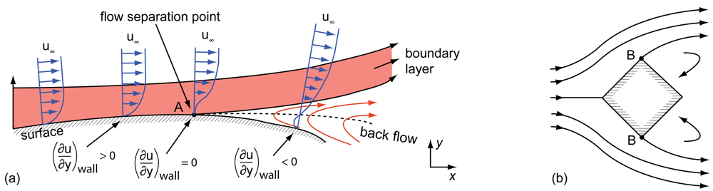
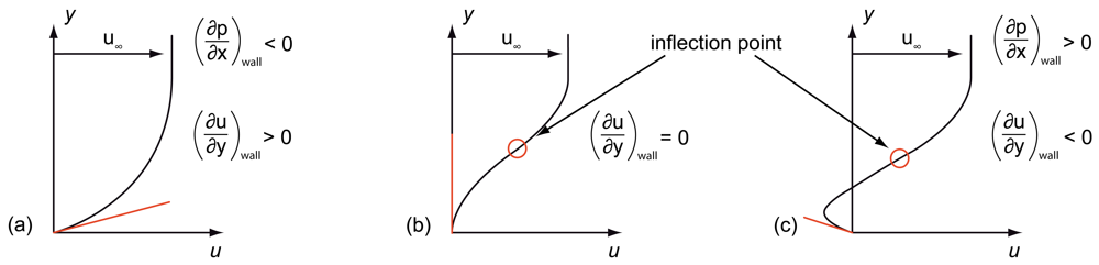
When flow separation occurs on a certain surface, the velocity boundary layer becomes detached from it, leading to unsteady flow conditions [2–4]. The phenomenon can basically be explained by the pressure conditions existing on the surface [4]: Figure 1(a) shows an airfoil within a certain flow. When a fluid particle reaches the airfoil's profile at the front (side facing the flow), it will be redirected and therefore accelerated up to a maximum velocity. From that velocity peak down to the trailing edge, the fluid is then decelerated again due to an increasing static pressure (region of adverse pressure gradient)—a behavior also known as pressure recovery or diffusion [5]. When assuming an inviscid flow—this can only be done at an adequate distance from the airfoil and its boundary layers—the pressure conditions can be approximated by Bernoulli's equation [6]: (1) ∇ → ( p stat + ρ 2 u 2 ) = 0where p_stat is the static pressure, ρ 2 u 2 the dynamic pressure and ∇⃗ the Nabla-operator ∇ → = ( ∂ ∂ x , ∂ ∂ y , ∂ ∂ z ). Considering the airfoil's profile in combination with Equation (1), it is assumed that a particle passing the airfoil has a constant total energy undergoing a transformation from high static (pressure) energy into high kinetic energy and back to static (pressure) energy again. The velocity of the particle in flow direction is thereby, of course, correlated to the kinetic energy leading to a low velocity at the front, a maximum velocity in the middle and a low velocity again at the airfoil's rear (side not facing the flow) [1–3].

When considering friction within the model, a certain amount of the fluid particles' total energy is lost leading to a lower kinetic energy. Thus, at certain flow conditions, there will be not enough kinetic energy of the fluid particles to counteract the increasing static pressure at the airfoil's rear. Especially fluid particles in the boundary layer suffering from the highest amount of friction will reduce their velocity to zero and start to follow a pressure gradient directed to the outer flow field. This pressure distribution leads to a movement in y-direction and even flow directed backwards to the overall flow direction [7,8].

Figure 1 illustrates two types of flow separation. However, both types can be led back to the same explanation above. The pressure based flow separation, shown in Figure 1(a), is caused by an adverse pressure gradient occurring at profiles without sharp edges (e.g., airfoil). In case of geometrical aberration (e.g., house wall), as shown in Figure 1(b), a flow separation is called geometrically-based [1,3].

A mathematical explanation of the flow separation background for the stationary case can be given by the Navier–Stokes equation [6]: (2) ( v → ⋅ ∇ → ) ⋅ v → + ∂ v → ∂ t = 1 ρ F → − 1 ρ ∇ → p + ν Δ v →with v⃗ = (u, v, w) as the field vector of velocity, ρ as density and ν as kinematic viscosity. F⃗ describes the amount of the external force per volume (force density per volume) and ∇_p the amount of the pressure force per volume in ^N/m³. νΔv⃗ represents the influence of friction within the equation where Δ = ( ∂ 2 ∂ x 2 + ∂ 2 ∂ y 2 + ∂ 2 ∂ z 2 ) is the Laplace operator [6].

For the following statements, all variables do not depend on the third coordinate z. Thus, z and w will further be neglected. If we now consider a position at the wall with y = 0, the definitions of the boundary layer give us a simplification with y = 0 and v⃗ = 0 (u = 0, v = 0). In a stationary case with ∂ v → ∂ t = 0, which is free of external forces with F⃗ = 0, Equation (2) can further be simplified to [7,9]: (3) 0 = − 1 ρ ∂ p ∂ x + ν ∂ 2 u ∂ y 2 .according to Equation (3), there are two important cases with ∂ p ∂ x < 0 and ∂ p ∂ x > 0, which can be distinguished here. The resulting flow profiles are illustrated in Figure 3.

The first case with ∂ p ∂ x < 0 results in ∂ 2 u ∂ y 2 < 0giving a negative curvature for u (y), meaning the slope of the function u (y) decreases for all values of y. Due to the fact that u (y) always tends to a positive value of u_∞, a trend of the function can be given, as illustrated in Figure 2(a): The figure shows the typical velocity distribution over y within a laminar boundary layer of an overflowed surface starting at u(0) = 0 to u (y ≫ 0) = u_∞[7–9]. In the second case the adverse pressure distribution ∂ p ∂ x > 0 results in a positive curvature with ∂ 2 u ∂ y 2 > 0, meaning the slope of the function u (y) has to increase first. Again at the end of the boundary layer a finite velocity of u_∞ has to be reached corresponding to a slope ∂ u ∂ y = 0. Therefore, the slope has to have a maximum value before it decreases again. The maximum value of the slope is also the inflection point of the function u(y). A further decrease of ∂ p ∂ xallows the possibility of [7,9]: (4) ∂ u ∂ y | wall = 0 ,which indicates the point of flow separation, as shown in Figure 2(b). Even negative values are possible, as shown in Figure 2(c), indicating back flow after flow separation [7,9].

The results from the Navier–Stokes equation showed the possibility of a flow separation on an overflowed surface. It will now be analyzed whether the phenomenon of reattachment of the boundary layer can be interpreted in the same way.

When flow separation occurs, the presence of an either laminar or turbulent flow condition will be essential for the developed flow profile, especially the presence of a flow reattachment and separation bubble formation. According to Schlichting, the current state of the flow conditions can be calculated by the Reynolds number [2]. A critical value of (5) Re crit = u ∞ l ν ≈ 5 ⋅ 10 5 ,with l as characteristic length shows the approximated transition between laminar (< 5 × 10⁵) and turbulent (> 5 × 10⁵) flow conditions of an overflowed flat plate. A precise value cannot be given here, since the real flow conditions depend on the airfoil's shape and roughness, pressure distribution and further factors [7,10,11].

At Reynolds numbers of 10⁴ or lower—implicating clear laminar flow conditions on an overflowed flat plate—a separated flow shows reattachment under certain circumstances (adverse pressure gradient) only. Having those laminar conditions (meaning we expect a laminar boundary layer), flow separation usually occurs instantly since laminar boundary layers can handle only small adverse pressure gradients without separation [7,8]. When assuming Reynolds numbers of 10⁶ or higher—implicating clear turbulent flow conditions on an overflowed flat plate—the characteristics of the separation are different to the laminar ones. Here, separation usually occurs with very high angles from the trailing edge moving forward with increasing incidence [7,8].

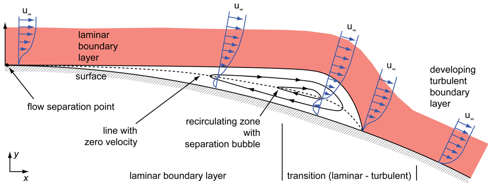
Other flow conditions show up for Reynolds numbers in the range between 10⁴ and 10⁶. Here, a separated flow also occurs, which is continuing along a tangent of the surface at the point of flow separation, as shown in Figure 3. The separated flow descends into a transition from laminar to turbulent flow forming a separation bubble. This phenomenon occurs often at those conditions and can be led back to the increasing distance of the boundary layer to the surface, which results in a higher transition susceptibility [7,8]. According to Gad-el-Hak, turbulent entrainment forces the flow back to the surface, causing the mentioned separation bubble [7].

Figure 3 illustrates a typical airfoil setup with an occurring flow separation followed by a reattachment. The figure shows the velocity profile on an airfoil's surface with the recirculating zone inside the separation bubble. As it can be concluded from Figure 3, a measurement of the actual flow at the separation point and point of reattachment should be possible by a measurement of zero flow in x-direction for y close to the wall. Due to Equation (4), this condition is fulfilled close to the separation and reattachment point only.

In the following, a measurement setup is presented quantifying the actual mean flow profile in x direction for y close to the wall, giving us the chance to determine either the point of separation or reattachment.

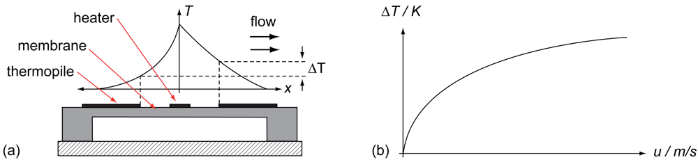
The thermal flow sensor consists of a heater and thermoelectric temperature sensors symmetrical to both sides of the heater. For thermal isolation, all parts are placed on a membrane. In operating mode, the heater will be heated up giving thermal energy to its surrounding, which is detected by both temperature sensors in the same way. In case of zero flow, the temperature distribution on the membrane will be symmetric, leading to the same detected temperature and therefore to no temperature difference between both thermopiles [17,18]. A presence of a fluid flow over the membrane lateral to the heater—as depicted in Figure 4(a)—causes an asymmetric temperature distribution leading to a measurable temperature difference between both temperature sensors. So, the temperature difference can be interpreted as a flow [18,19].

There are different ways of operating the heater as well as different kinds of temperature sensors possible. In most cases, a constant current (CC) or constant power (CP) is used as operational mode for the heater due to its simplicity. A constant temperature mode (CT) is also used by controlling the heater's temperature-dependent electrical resistance. The effort of realizing a CT mode is higher but it comes along with a higher detectable flow range of the sensor [19,20]. The temperature sensors can be resistive or based on the thermoelectric effect (thermopiles) [21]. When using thermopiles, the thermoelectric effect is converting a temperature difference ΔT directly into a voltage (6) U AB = α AB ⋅ Δ T ,where α_AB represents the relative Seebeck coefficient of the used thermopile materials A and B. More information about this topic can be found in [21]. Figure 4(b) shows the characteristic line of a thermal flow sensor in combination with a thermopile-based measurement. As already mentioned, the temperature difference is used for measurement demonstrating the differential principle of the sensor. The principle comes along with a reduction of cross sensitivities and therefore a higher reproducibility of the sensor signal. Furthermore, the output signal of a thermopile-based measurement is baseline free when compared with state-of-the-art resistive approaches on boundary layer detection [12,13,16,22]. Therefore, this approach has been chosen as basic measurement principle for the measurements presented further down.

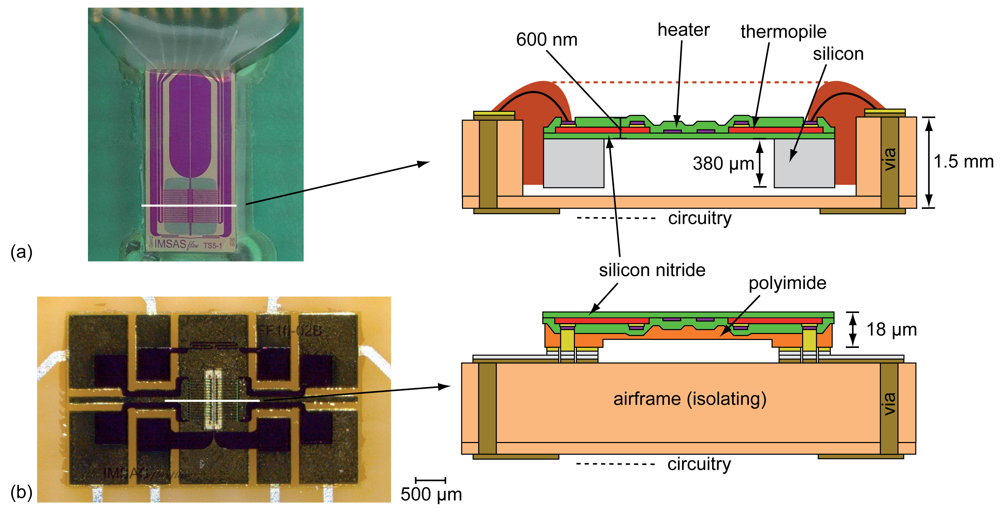
As already mentioned, the flow sensor used in this work consists of a combination of heater and thermopiles placed on a membrane [21]. The thermopiles consist of an in-situ doped polysilicon and an alloy of 90% tungsten and 10% titanium (WTi). For the heater the WTi alloy has also been used. Both functional elements are embedded in a 600 nm thin membrane made of silicon-rich low-stress LPCVD (low pressure chemical vapor deposition) silicon nitride (SiN). The membrane material deposition with its low tensile stress of +200 MPa has been designed for achieving a high mechanical stability only. A high chemical and thermal stability is also given since the SiN membrane deposition on the functional layers (passivation) is done as LPCVD process at 800 °C. This could be achieved due to diffusion barriers of titanium nitride (TiN) between the polysilicon and WTi used in the thermopile process. More detailed information about the whole process concerning the non-flexible flow sensor can be found in Buchner et al. [21]. For the flexible approach, the 380 μm silicon substrate is replaced by a 18 μm thick polyimide. The whole transfer process is shown in [23,24].

Due to its high importance for the aviation sector, an integration of thermal flow sensors has been done on airfoils. As it can be seen in Figure 5, there are two basic concepts of flow sensors used in the following experimental setup.

Figure 5(a) shows an integrated silicon based thermal flow sensor and a schematic of its cross-sectional view. Except for the bond wires (electronic contacting), the whole sensor has been flush-mounted to avoid turbulences on steps that could disturb the measurements. The electronic contacting by bond wires is—due to its height—placed far away from the measuring part of the sensor. As it can be seen, a flush mounting of a silicon-based thermal flow sensor needs another cavity for placing the sensor in addition to the vias for electric contacting, which always affects the structural health of the wing. Therefore, a second approach with a thin flexible polyimide substrate has been developed. Figure 5(b) shows that this approach does not need a second cavity due to its flip chip contacting in combination with its small height. A more detailed overview of both sensor integration processes can be found in [21,23,24].

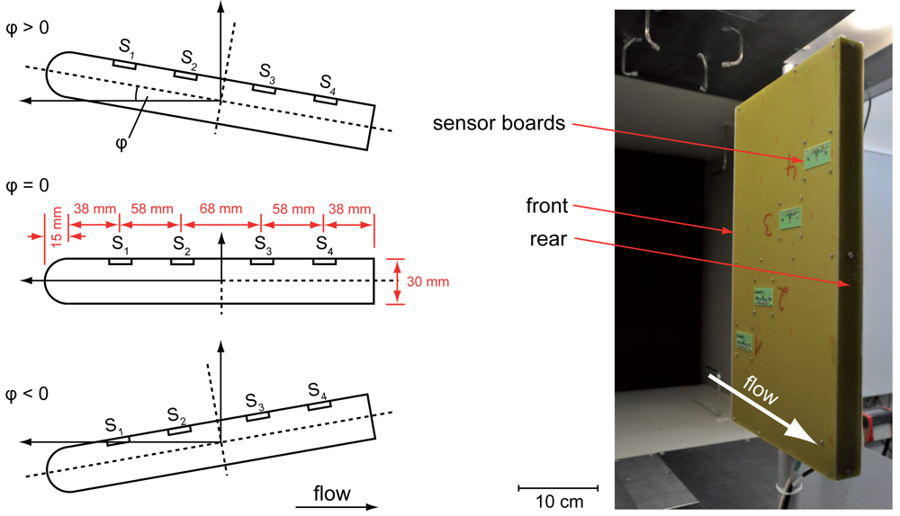
To evaluate the feasibility of flow separation/reattachment detection by the presented sensing elements, a series of four elements has been integrated on an airfoil. Printed circuit boards have been used for higher adaptability in integration. Those boards have a size of 5 cm × 2.5 cm and can directly be flush-mounted on the airfoil's surface avoiding any steps in flow direction. This gives us the chance to use different flow sensor types with exactly the same measurement setup.

All measurements have been performed in a closed loop wind tunnel at Deutsche WindGuard Wind Tunnel Services GmbH. Figure 6 (right) shows the whole measurement setup. As shown in Figure 6 (left), the cross section is directed with the round-shaped side facing the flow to get a preferably low fluidic resistance. A heater power of 15 mW has been chosen, while the whole sensor setup is running in constant voltage mode. The sampling rate is set to 1 kHz with an averaging in a time interval of 1 s. Sampling, measurement and calculations are made with a National Instruments USB-6212 digital acquisition card combined with LabView.

The sensor signals shown in the following are always normalized, meaning a normalization run has been done at defined flow rates to show the existing difference of the thermopile signals for different sensors. Those slight differences are caused by inaccuracies during the sensor fabrication process and cannot be avoided completely. The adaption is small, but for having the right nomenclature, all sensor signals are marked as mV(n) (normalized) instead of mV.

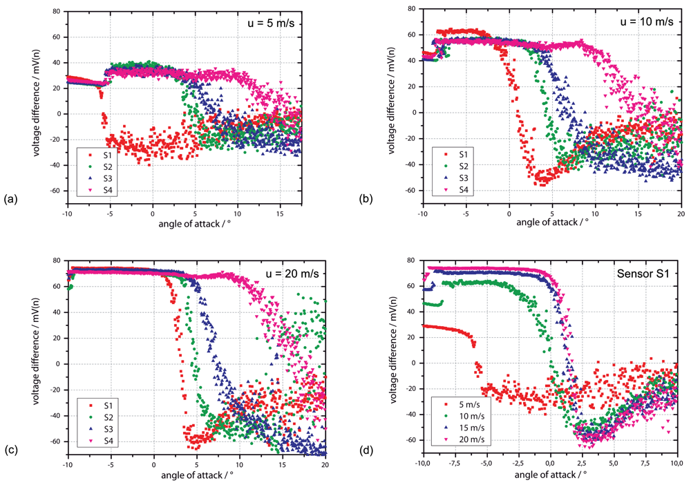
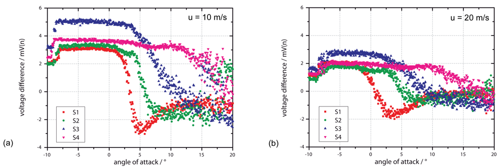
In the first measurement, the signals of four equidistantly placed flow sensors (see Figure 6 for exact position) are recorded for constant wind speeds and different angles of attack (φ, also pitch) between −10° and +20°. How φ is defined can be seen in Figure 6 (right). Figure 7 shows the sensor signals of S₁, S₂, S₃ and S₄ averaged over a time interval of 1 s at wind speeds of 5 m/s (a), 10 m/s (b) and 20 m/s (c). In Figure 7(d) the flow signals of S1 to be compared at different wind speeds are selected only. The resulting graphs show basically the same characteristics for all wind speeds: A constant positive output signal always exists at the starting point with φ = −10°. With increasing angle S₁ followed by S₂, S₃ and S₄, the output signals decrease down to zero ending up in negative values with high standard deviation. According to the definitions from Section 3, an output signal of zero shows a vanishing flow velocity in x-direction for small values of y (close to the wall), a result that could be led back to a flow separation [7,8]. An argument supporting the approach of a pressure-based flow separation is the decreasing output signal, which might occur due to back flow. In contrast, the high noise that can be observed after zero crossing and the sequence of the sensors from S₁ to S₄ do not fit into the scheme. If a flow separation with back flow occurs at S₁, there should definitely be an impact to all following sensors S₂ to S₃. This cannot be observed here, leading to the second possibility of a reattachment of the flow.

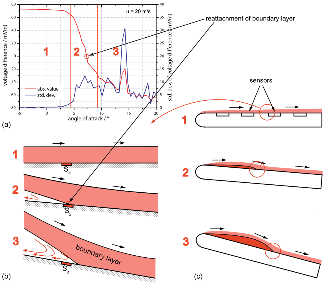
To introduce the idea of an observed reattachment of the flow, we should consider Figure 8. Figure 8(a) shows the results of sensor S3 only for different angles of attack as a mean value out of ten seconds as well as the standard deviation of the signal. The output signal shows a clear and constant positive signal in flow direction for φ < 3° with a standard deviation of 0.2 mV. With higher angles 3° < φ < 7° the flow signal decreases to zero and further down where the standard deviation shows a clear increase. When considering the possibility of a reattachment of the flow passing through, those conditions can be assumed in the same way as shown in Figure 8(b,c) [7,8]. In this assumption, a separation bubble occurs starting at the front of the airfoil, which is rising with increasing angle of attack. With this approach the mentioned problem of the sensor sequence S₁ to S₄ does not occur. Furthermore, the high scattering after zero crossing in Figure 7 and therefore the increase in standard deviation in Figure 8 can be explained: The turbulent conditions increase the integral time scale of the flow, which reduces the independent number of samples acquired.

According to Section 1.2, the phenomenon of an occurring separation bubble expects a Reynolds number between 10⁴ and 10⁶[1,7,25]. When working with flow rates between 5 m/s and 20 m/s, the Reynolds numbers can be determined using Equation (5) to values between 7.5 × 10⁴ and 3 × 10⁵. The results show that a reattachment due to a transition from laminar to turbulent flow as described in Section 1.2 is possible. Accordingly, the separation itself occurs between the first sensor S₁ and the front of the airfoil. A simple experiment observing this issue is the use of a wool thread showing the direction of the actual flow at each designated position: The experiment indicates a geometric flow separation right at the front of the airfoil forming a separation bubble with backflow close to the airfoil's wall. As measured with the thermal flow sensors, the backflow is characterized by a high standard deviation. After the reattachment point, the wool thread always shows a clear flow direction down to the rear.

It is to be mentioned that the behavior of the first sensor S₁ at 2 m/s and 5 m/s, as depicted in Figure 7 and Figure 9, shows a zero flow for a negative angle of attack. There are three possibilities to explain the observed behavior, including the unintended detection of a stagnation point, flow separation point or a reattachment as it occurs on all other sensors. The detection of a stagnation point can be eliminated due to the observed signal trend, which would be negative for higher angles, and vice versa, since the stagnation point has to pass through from rear to front for increasing angles. Here the characteristics are exactly inverted. A detection of a boundary layer separation can also be eliminated, since this would have an effect on the sensor signals of S₂, S₃ and S₄. The most probable reason for the observed sensor behavior of S₁ is a reattachment as well, which also occurs due to a flow separation at the airfoil's front. Flow separation is not expected for this setup, but here it has to be taken into consideration that the used airfoil is not a perfectly flat plate but a structure having a thickness of 30 mm. At lower flow velocities, the flow could have been redirected showing this phenomenon with a reattachment afterwards.

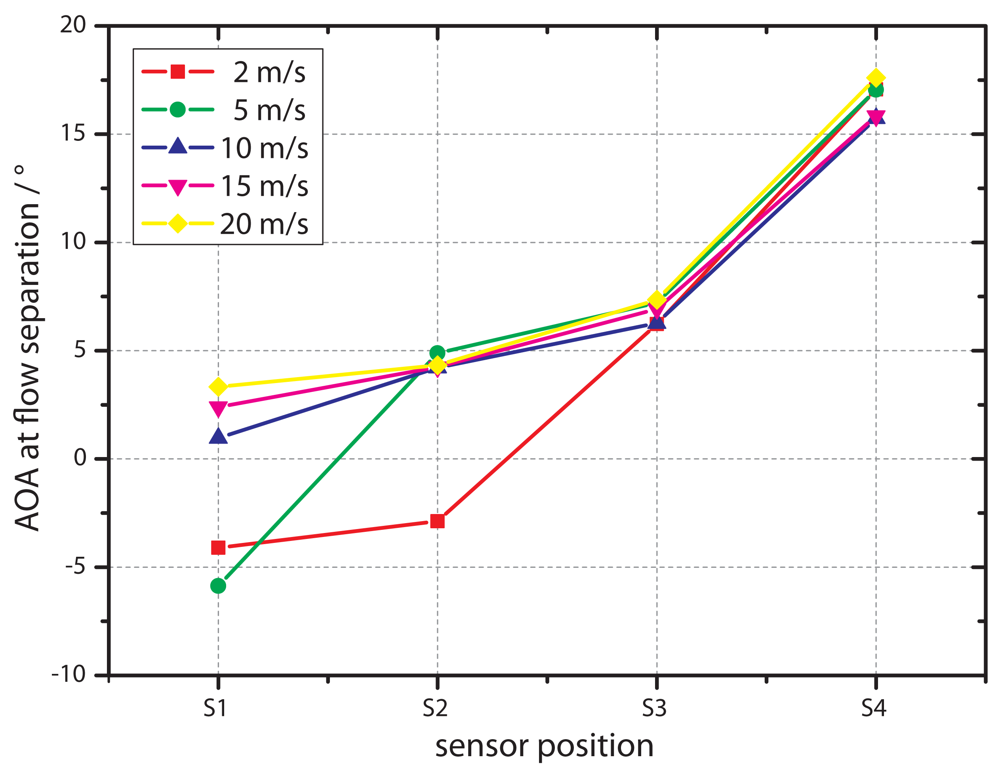
Figure 9 shows the relationship between the angle of attack at zero output and the position of the sensors for flow velocities of 2 m/s, 5 m/s, 10 m/s, 15 m/s and 20 m/s. It illustrates that for the sensors positioned in the back of the airfoil, the AOA at the point of reattachment is equal for all flow velocities. As already mentioned, at S₁ and S₂ differences of the AOA to the sensors in the rear can be observed, especially at lower flow rates of 2 m/s and 5 m/s. Here, even negative values have been measured, giving a further argument that the zero crossing of the AOA is caused by a reattachment. It should be mentioned that the reattachment position at S₃ and S₄ is not sensitive to the flow velocity and, thus, to the Reynolds number. S₃ and S₄ are already close to the rear of the airfoil. Due to that influence, the usual dependency between Reynolds number and length of separation bubble will be different. A lack of accuracy from the data acquisition can be excluded here, since the points of reattachment are easy to identify (low scattering), as shown in Figure 7. A more probable reason is the selected airfoil with its overall length in flow direction of 260 mm and its profile in general.

Another measurement has been done using thermal flow sensors based on thin flexible substrates. To get a good comparison between both sensor types, the same setup has been used.

As shown in Figure 10(a,b), the measured flow characteristics are comparable with the silicon-based sensors. Differences can be seen when considering the absolute signal: here the sensors show a lower reproducibility as well as a lower output signal. The lower reproducibility is derived from the integration process, which has a higher influence on the characteristic line of a flexible approach rather than a non-flexible approach. A lower output signal of the flexible approach comes from the additional polyimide layer as part of the membrane: The polyimide layer increases the heat flux through the membrane, leading to a lower percentage of heat flux going through the fluid. Thus, the sensing element loses sensitivity, but the detection of a flow separation and reattachment is still possible.

References

- Greenblatt, D.; Wygnanski, I.J. The Control of Flow Separation by Periodic Excitation. Prog. Aerosp. Sci. 2000, 36, 487–545. [Google Scholar]
- Schlichting, H.; Gersten, K.; Krause, E. Grenzschicht-Theorie, 10th ed.; Springer-Verlag: Berlin/Heidelberg, Germany, 2006; pp. 377–408. [Google Scholar]
- Bohl, W.; Elmendorf, W. Technische Strömungslehre, 14th ed.; Vogel-Fachbuch: Würzburg, Germany, 2008; pp. 260–302. [Google Scholar]
- Chang, P.K. Separation of flow. J. Franklin Inst. 1961, 272, 433–448. [Google Scholar]
- Johnson, R.W. The Handbook of Fluid Dynamics; CRC Press: Boca Raton, FL, USA, 1998. [Google Scholar]
- Stöcker, H. Taschenbuch der Physik, 5th ed.; Verlag Harri Deutsch: Frankfurt am Main, Germany, 2007. [Google Scholar]
- Gad-el Hak, M. Flow Control-Passive, Active, and Reactive Flow Management, 1st ed.; Cambridge University Press: Cambridge, UK, 2000; pp. 150–203. [Google Scholar]
- Genc, M.S.; Karasu, I.; Acikel, H.H.; Akpolat, M.T. Low Reynolds Number Flows and Transition. In Low Reynolds Number Aerodynamics and Transition; Genc, M.S., Ed.; InTech: Rijeka, Croatia, 2012; pp. 1–28. [Google Scholar]
- Christy, J. U01668 Fluid Mechanics (Chemical) 4. Available online: http://www.see.ed.ac.uk/johnc/teaching/fluidmechanics4/ (accessed on 22 October 2012).
- Aubertine, C.D.; Eaton, J.K.; Song, S. Parameters Controlling Roughness Effects in a Separating Boundary Layer. Int. J. Heat Fluid Flow 2004, 25, 444–450. [Google Scholar]
- Crabtree, L. The Formation of Regions of Separated Flow on Wing Surfaces; Aeronautical Research Council: London, UK.
- Liu, K.; Yuan, W.; Deng, J.; Ma, B.; Jiang, C. Detecting Boundary-layer Separation Point with a Micro Shear Stress Sensor Array. Sens. Actuators A: Phys. 2007, 139, 31–35. [Google Scholar]
- Jiang, F.; Lee, G.B.; Tai, Y.C.; Ho, C.M. A Flexible Micromachine-based Shear-stress Sensor Array and its Application to Separation-point Detection. Sens. Actuators A: Phys. 2000, 79, 194–203. [Google Scholar]
- Guo, S.; Lai, C.; Jones, T.; Oldfield, M.; Lock, G.; Rawlinson, A. The Application of Thin-film Technology to Measure Turbine-vane Heat transfer and Effectiveness in a Film-cooled, Engine-simulated Environment. Int. J. Heat Fluid Flow 1998, 19, 594–600. [Google Scholar]
- Spencer, M.; Jones, T.; Lock, G. Endwall Heat Transfer Measurements in an Annular Cascade of Nozzle Guide Vanes at Engine Representative Reynolds and Mach Numbers. Int. J. Heat Fluid Flow 1996, 17, 139–147. [Google Scholar]
- Buder, U.; Petz, R.; Kittel, M.; Nitsche, W.; Obermeier, E. AeroMEMS Polyimide Based Wall Double Hot-wire Sensors for Flow Separation Detection. Sens. Actuators A: Phys. 2008, 142, 130–137. [Google Scholar]
- Ashauer, M.; Glosch, H.; Hedrich, F.; Hey, N.; Sandmaier, H.; Lang, W. Thermal Flow Sensor for Liquids and Gases. Proceedings of the Eleventh Annual International Workshop on Micro Electro Mechanical Systems (MEMS), Heidelberg, Germany, 25–29 January 1998; pp. 351–355.
- Ashauer, M.; Glosch, H.; Hedrich, F.; Hey, N.; Sandmaier, H.; Lang, W. Thermal Flow Sensor for Liquids and Gases Based on Combinations of Two Principles. Sens. Actuators A: Phys. 1999, 73, 7–13. [Google Scholar]
- Van Oudheusden, B. Silicon Thermal Flow Sensors. Sens. Actuators A: Phys. 1992, 30, 5–26. [Google Scholar]
- Löfdahl, L.; el Hak, M.G. MEMS Applications in Turbulence and Flow Control. Prog. Aero. Sci. 1999, 35, 101–203. [Google Scholar]
- Buchner, R.; Sosna, C.; Maiwald, M.; Benecke, W.; Lang, W. A High-temperature Thermopile Fabrication Process for Thermal Flow Sensors. Sens. Actuators A: Phys. 2006, 130–131, 262–266. [Google Scholar]
- Haasl, S.; Stemme, G. Flow sensors. In Comprehensive microsystems; Gianchandani, Y.B., Tabata, O., Zappe, H., Eds.; Elsevier: Amsterdam, The Netherlands, 2008; pp. 209–272. [Google Scholar]
- Sturm, H. Thin Chip Flow Sensors for Nonplanar Assembly. In Ultra-thin Chip Technology and Applications; Burghartz, J.N., Ed.; Springer: New York, NY, USA, 2011; pp. 377–387. [Google Scholar]
- Buchner, R.; Froehner, K.; Sosna, C.; Benecke, W.; Lang, W. Toward Flexible Thermoelectric Flow Sensors: A New Technological Approach. J. Microelectromech. Syst. 2008, 17, 1114–1119. [Google Scholar]
- Darabi, A.; Wygnanski, I. Active Management of Naturally Separated Flow Over a Solid Surface. Part 1. The Forced Reattachment Process. J. Fluid Mech. 2004, 510, 105–129. [Google Scholar]
- Gould, D.; Sturm, H.; Lang, W. Thermoelectric Flow Sensor Integrated Into an Inductively Powered Wireless System. IEEE Sens. J. 2012, 12, 1891–1892. [Google Scholar]
- Burghartz, J.; Appel, W.; Rempp, H.; Zimmermann, M. A New Fabrication and Assembly Process for Ultrathin Chips. IEEE Trans. Electron Devices 2009, 56, 321–327. [Google Scholar]
- Burghartz, J.N.; Appel, W.; Harendt, C.; Rempp, H.; Richter, H.; Zimmermann, M. Ultra-thin Chip Technology and Applications, a New Paradigm in Silicon Technology. Solid State Electron 2010, 54, 818–829. [Google Scholar]
© 2012 by the authors; licensee MDPI, Basel, Switzerland. This article is an open access article distributed under the terms and conditions of the Creative Commons Attribution license (http://creativecommons.org/licenses/by/3.0/).
Share and Cite
Sturm, H.; Dumstorff, G.; Busche, P.; Westermann, D.; Lang, W. Boundary Layer Separation and Reattachment Detection on Airfoils by Thermal Flow Sensors. Sensors 2012, 12, 14292-14306. https://doi.org/10.3390/s121114292
Sturm H, Dumstorff G, Busche P, Westermann D, Lang W. Boundary Layer Separation and Reattachment Detection on Airfoils by Thermal Flow Sensors. Sensors. 2012; 12(11):14292-14306. https://doi.org/10.3390/s121114292
Chicago/Turabian StyleSturm, Hannes, Gerrit Dumstorff, Peter Busche, Dieter Westermann, and Walter Lang. 2012. "Boundary Layer Separation and Reattachment Detection on Airfoils by Thermal Flow Sensors" Sensors 12, no. 11: 14292-14306. https://doi.org/10.3390/s121114292