Reconstruction of Self-Sparse 2D NMR Spectra from Undersampled Data in the Indirect Dimension †


Abstract
: Reducing the acquisition time for two-dimensional nuclear magnetic resonance (2D NMR) spectra is important. One way to achieve this goal is reducing the acquired data. In this paper, within the framework of compressed sensing, we proposed to undersample the data in the indirect dimension for a type of self-sparse 2D NMR spectra, that is, only a few meaningful spectral peaks occupy partial locations, while the rest of locations have very small or even no peaks. The spectrum is reconstructed by enforcing its sparsity in an identity matrix domain with ℓp (p = 0.5) norm optimization algorithm. Both theoretical analysis and simulation results show that the proposed method can reduce the reconstruction errors compared with the wavelet-based ℓ1 norm optimization.
1. Introduction
Nuclear magnetic resonance (NMR) spectroscopy is widely utilized to analyze the structures of chemicals and proteins. Multidimensional NMR spectra can provide more information than one-dimensional (1D) NMR spectra. The acquisition time for a conventional two-dimensional (2D) NMR spectrum is mostly determined by the number of t1 increments in the indirect dimension. One possible way is to reduce the acquisition time is to reduce the number of t1 increments. However, this will result in aliasing of the spectrum in the indirect dimension [1,2], because the sampling rate is lower than the requirement of the Nyquist sampling rule.
Researchers have been seeking ways to suppress the aliasing from the aspects of sampling and reconstruction. Radial sampling presents relatively small leakage artifacts [3] and Poisson disk sampling is observed to provide a large low-artifact area in the signal vicinity [4]. The maximum sampling time for multi-dimensional NMR experiments was analyzed by Vosegaard and co-workers [5]. Besides the sampling patterns, some reconstruction algorithms have been employed to improve spectral quality, including maximum entropy [6,7], iterative CLEAN algorithm [8] and Bayesian reconstruction [9]. The sparse sampling was incorporated with intermolecular multiple-quantum coherences for high-resolution 2D NMR spectra in inhomogeneous fields [10].
Recently compressed sensing (CS) theory [11,12], for reconstructing signals from fewer numbers of measurements than the number that the Nyquist sampling rule requires has attracted lots of attention in medical imaging [13], single pixel imaging [14], and computer vision [15], etc. Under the assumption that the acquired data is sparse or compressible in a certain sparsifying transform domain, CS can successfully recover the original signal from a small number of linear projections with little or no loss of information. The choice of sparsifying transform is important in the CS. The sparsfying transform should be maximally incoherent with the measurement operator. Intuitively, the target signal should be sparsely represented in the transform domain, e.g., wavelet transform domain, and this spare representation should be spread out in the encoding scheme. Iddo introduced CS to reconstruct a 2D NMR spectrum from partial random measurements of its time domain signal under the assumption that the spectrum is sparse in the wavelet domain [16].
In this paper, we focus on the reconstruction of self-sparse NMR spectra, that is, a few meaningful spectral peaks occupy partial locations while the rest locations have very small or even no meaningful peaks. NMR spectra includes regions where no signals arise because of the discrete nature of chemical groups [17]. The reason we pay attention to self-sparse NMR spectra is that many NMR spectra of chemical substances fall in this type [3,10,16,17]. Based on the concept of sparsity and coherence in CS, we demonstrate that a wavelet transform is not necessary to sparsify the self-sparse NMR spectra or even worsens the reconstruction. We propose to reconstruct the NMR spectrum by enforcing its sparsity in an identity matrix domain with a ℓp (p = 0.5) norm optimization algorithm. Simulation results show that the proposed method can reduce the reconstruction errors compared with the wavelet-based ℓ1 norm optimization.
Recently, Kazimierczuk and Orekhov [18] and Holland et al. [19] independently proposed to use CS in proton NMR and showed promising results in reducing acquired data. A combination of spatially encoding the indirect domain information and CS was proposed by Shrot and Frydman [20]. The spectra were considered to be sparse themselves [18–20], differing from the sparse representation using wavelets [16]. However, no comparison on the reconstructed spectra with and without wavelet transform was given and no theoretical analysis was presented. In this paper, we will analyze the performance of wavelet transform in the CS-NMR basing on the sparsity and coherence properties and simulated results.
The remainder of this paper is organized as follows. In Section 2, the reason to undersample the indirect dimension is given by calculating the acquisition time for a 2D NMR spectrum. In Section 3, the two key factors of CS, sparsity and coherence, are briefly summarized and their values are estimated for 2D spectra, followed by the proposed reconstruction method. In Section 4, reconstruction of self-sparse NMR spectra is simulated to show the shortcomings of the wavelet and the advantage of the identity matrix. The improvement of utilizing the ℓp norm is also demonstrated. Finally, discussions and conclusions are given in Section 5.
2. Undersampling in the Indirect Dimension of 2D NMR
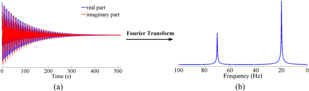
In NMR spectroscopy, a typical sampled noiseless time domain signal can be described as a sum of exponentially decaying sinusoids:
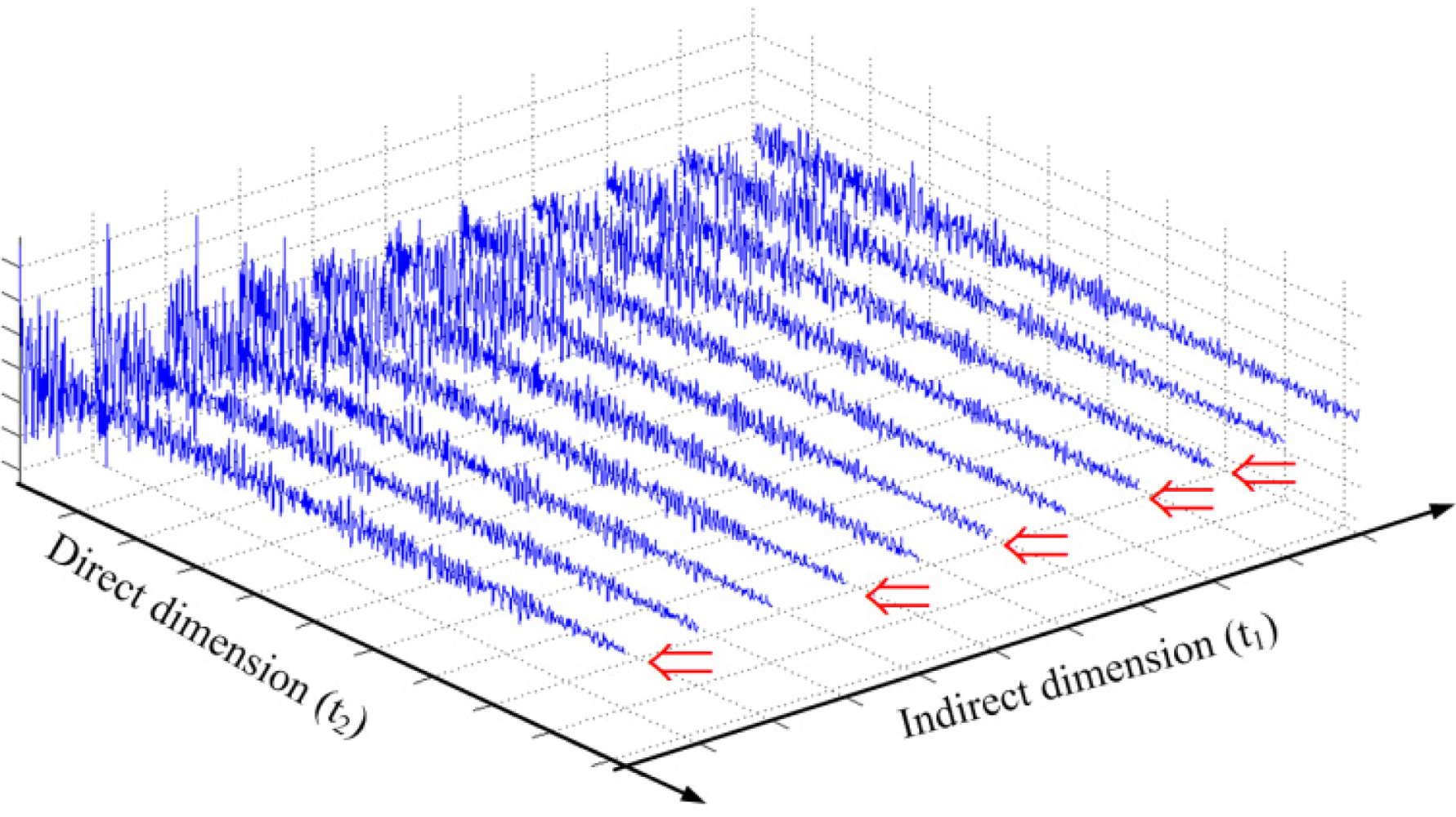
The typical experimental time for a 1D NMR spectrum usually takes several seconds, thus it is not time consuming. However, for a 2D NMR spectrum, the time domain signal is generated based on two time variables t1 and t2. As shown in Figure 2, one scan of 2D NMR spectrum contains three steps: first, the sample is excited by one or more pulses in the preparation period. These pulses result in the evolution of magnetization with time t1; then, the sample is further excited in the mixing period; finally, an FID signal is recorded as a function of t2. Usually, t1 is set as t1 = Δt1, 2Δt1, ..., n1Δt1, N1Δt1 (The increment Δt1 is usually at the order of milliseconds). The number of t1 increments (N1) is determined by:
Finally, 2D FT is performed on the 2D FID data. If the time for performing all the pulses in one scan is tp, the total scanning time for a 2D NMR spectrum will be:
In order to obtain a good resolution in the indirection dimension, N1 is usually several tens or hundreds or even more. This will cause the total scanning time for a 2D NMR spectrum to be tens of minutes or even several hours [22–26].
In this paper, we aim to reduce the scan number for the t1 dimension. Rather than using the uniform increment in the indirect dimension (t1 = Δt1, 2Δt1, ..., n1Δt1, N1Δt1), we randomly choose unduplicated Q numbers from nq ∈ {1, 2, ..., N1}, and let t1 = nqΔt1. Let:
The approximation is made by ignoring the total evolution time ∑nq∈ {1,2,...,N1},q = 1,2,...,QnqΔt1 since this value is only in the order of seconds. Compared to the time to acquire a 2D spectrum with fully sampled FIDs in the indirection dimension, undersampling the FIDs in the indirect dimension can greatly reduce the acquisition time for a 2D NMR spectrum if ρ is small enough. Figure 3 shows an example where we randomly undersample the indirect dimension with sampling rate ρ = 5/11 = 0.45. It means we save nearly half of the acquisition time of the conventional scheme.
However, this undersampling will result in aliasing artifacts [1,6]. It would be of great value if we can minimize these artifacts and reconstruct the full 2D NMR spectrum from the limited data. Here we explore the undersampling and reconstruction methods under the framework of CS.
3. Reconstruction of 2D Self-Sparse NMR Spectra with Compressed Sensing
3.1. Basic Concepts in Compressed Sensing
The CS proposed by Candès et al. [11] and Donoho [12] is a new theory to do undersampling and reconstruct the signal of interest from limited physically acquired data. They build a theoretical foundation that one can exactly or approximately recover signals from highly incomplete measurements. The two basic tenets to guarantee the performance of CS are sparsity and incoherence.
(a) Sparsity. For the signal x ∈ RN and a basis dictionary Ψ ∈ RS × N (e.g., identity matrix, FT, discrete cosine transform or wavelet transform matrix), the sparsity is often interpreted as:
Candès et al. [11] and Donoho [12] proved that it is possible to recover the original signal x from O(NlogS) measurements. This means the required number of measurements is proportional to the number of nonzero entries in the basis Ψ. The smaller the S is, the less the number of measurements is required.
(b) Incoherence. When a signal x is sampled by a sensing matrix ΦM × N, the measurements y ∈ RM of x is:
The coherence is defined as [27,28]:
If the signal x satisfies [30]:
The recovered signal is:
Equation (9) implies that if the coherence between Φ and Ψ is small, more non-zeros can be allowed in the sparse representation α. CS suggests Φ to be random enough to guarantee its incoherence with any Ψ. This is also observed that random sampling in time domain can improve the quality of reconstructed spectra [31].
However, ℓ0 norm is known to be intractable and sensitive to noise [11,12], and ℓ1 norm convex optimization is commonly used in CS to recover x by solving:
The accuracy of CS reconstruction using Equation (12) can be guaranteed if ΦΨ satisfies the appropriate restricted isometry properties [32]. A restricted isometry constant σs [32] defined as the smallest number such that:
The number of measurements M should satisfy:
Iddo [16] applied CS to remove the aliasing artifacts from incompletely acquired FID data by enforcing the sparsity of 2D NMR spectra in wavelet domain according to:
In this paper, we focus on the reconstruction of self-sparse NMR spectra in which significant peaks take up partial locations of the full NMR spectra while the remaining locations have very small or even no peaks. Ideally, if the number of sinusoids J in Equation (1) is very small, and the meaningful peaks are narrow enough relative to the whole 2D frequency coverage, the spectra can be considered to be sparse since the number of non-zeros for the spectra is much smaller than the number of spectrum points in the 2D NMR spectra.
The sparsifying transform and the coherence between Ψ and Φ = ΘFT play important roles in the CS, as we have discussed. In the following sections, we will demonstrate that wavelet is not necessary to sparsify or even worsens the self-sparse NMR spectra based on the concept of sparsity and coherence. We will then reconstruct the NMR spectrum by enforcing its sparsity in an identity matrix domain with ℓp (p = 0.5) norm optimization algorithm.
To represent the NMR spectra in conventional way [4–7,17], the X and Y coordinate axes are shown with unit of parts per million (ppm) [21] defined as:
3.2. Sparsity of Self-Sparse NMR Spectra
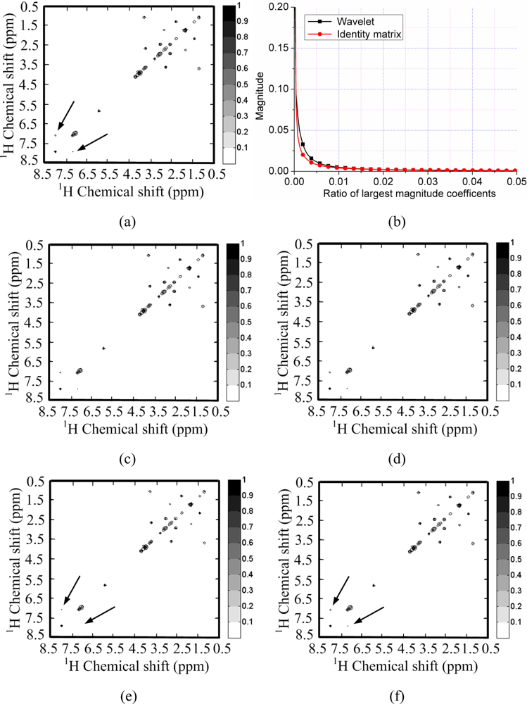
Figure 4(a) shows a 2D 1H-1H correlation spectroscopy (COSY) spectrum where most of the peaks fill partial and very limited regions of the full spectrum. This leads to the sparsity of spectrum because the number of non zeros in the 2D spectrum is much smaller than the number of spectrum points. This phenomenon is also observed by Yoh Matsuki et al. [17].
To test the sparsity of NMR spectra, we can measure the decay of coefficients in a sparsifying transform domain and evaluate the approximation error by retaining the k-term largest coefficients, because the reconstruction error is proportional to the power law decay k−r, where r is a constant implying the sparsity of signal [29]. Rapid decay of coefficients implies that one can use less non-zero coefficients to approximate a NMR spectrum. If we directly measure the decay of signal without complicated sparsifying transform, e.g., wavelets, it means measure the self-sparsity of signal. Mathematical saying is measuring its sparsity in the identity matrix.
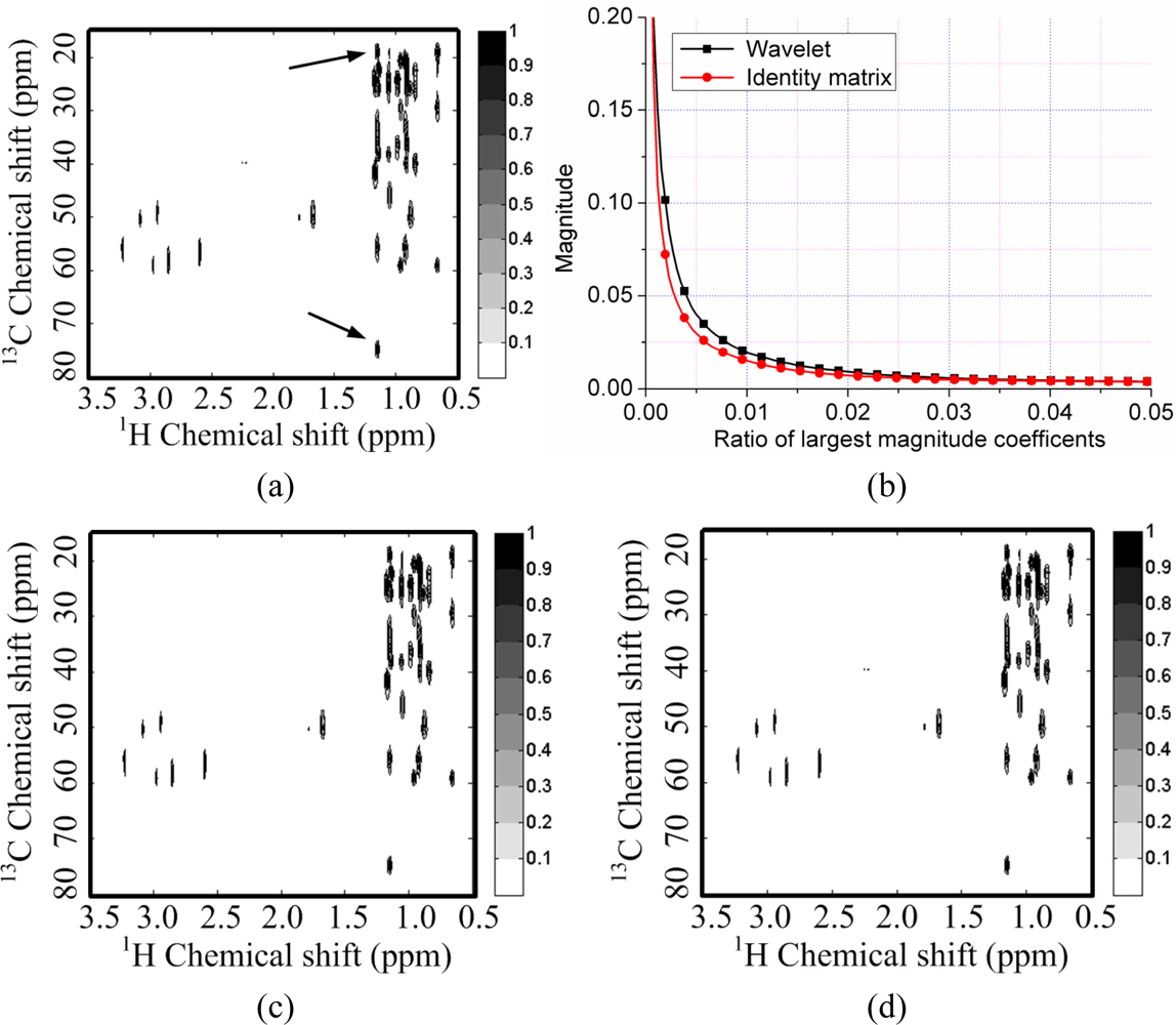
As shown in Figure 4(b), both the spectra and its wavelet coefficients can achieve rapid decay. By retaining 3% largest magnitude coefficients, the spectra can be reconstructed well in Figure 4(c,d). However, the spectrum is sparser than its representation in the wavelet domain. This is demonstrated by the faster decay of spectrum than that of its wavelet coefficients in Figure 4(b). By retaining the 1% largest magnitude coefficients, the wavelet fails to represent some peaks while the spectrum itself can represent these peaks, as marked by the arrows in Figure 4(e,f).
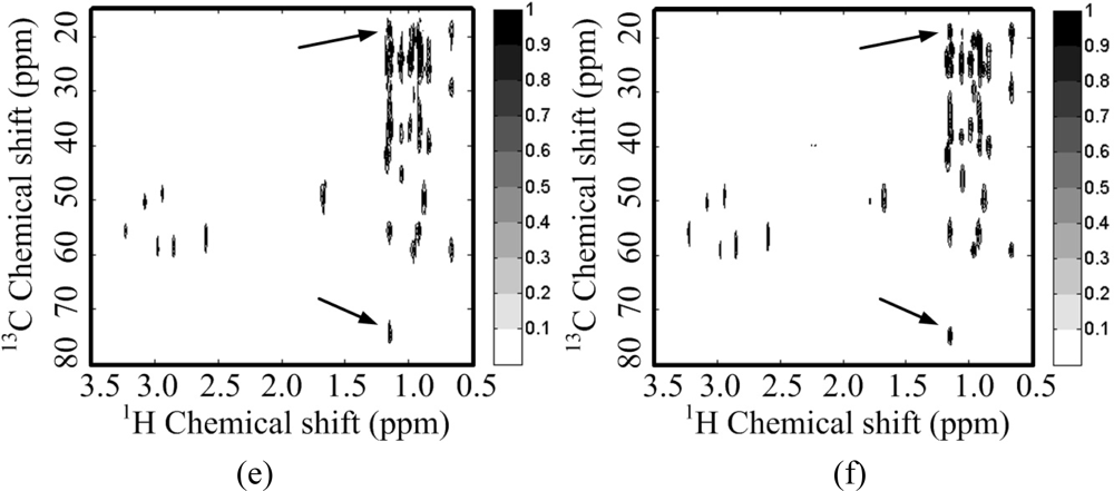
For a 2D 1H-13C COSY spectrum, the spectrum decays faster than its wavelet coefficients (Figure 5(b)). This implies that the identity matrix can provide a sparser representation of spectra than a wavelet does. Peaks are lost or distorted by using the wavelet transform to represent the spectrum (Figure 5(e)), but the spectrum is represented very well with the identity matrix (Figure 5(f)). This phenomenon is consistent with the observation on the 2D 1H-1H COSY spectrum discussed above.
As a result, this spectrum is self-sparse, which means spectrum is sparse in the identity matrix. Thus, according to Equations (9) and (14), it is better to use an identity matrix than to use a wavelet to reconstruct the self-sparse spectra from undersampled FIDs since the wavelet cannot provide a sparser representation of the spectrum. In fact, Stern et al. [33] proposed to do iterative soft thresholding on the spectrum directly, not on wavelet coefficients, to recover one dimensional NMR spectra from the truncated FIDs. Although the sparsity of NMR spectra is not explicitly expressed in that work [33], the recovered spectrum is obtained from minimizing ℓ1 norm of spectrum, which implies enforcing the sparsity of the spectrum. The problem of their method is that truncation violates the random sampling scheme in CS and results in strong Gibbs ringing which is hard to suppress [29]. What is more, truncating the 1D FID is not necessary to save the time to scan a spectrum since scanning a 1D NMR spectrum is fast and only takes on the order of seconds.
3.3. Coherence Property of Wavelet-Based and Identity Matrix-Based CS-NMR Spectra
Besides the sparsity of signal, another key factor for CS is the coherence between Φ and Ψ According to Equations (9) and (14), fewer measurements are required for signal sampling system Φ if it is less coherent with Ψ and the signal has same sparsity for different Ψ.
Pioneering work on CS has pointed out that the coherence of a time-frequency pair is μ(Φ, I) = μ(ΘFT, I) = 1 [28]. Thus, we only need to compute the coherence between undersampled Fourier operator Φ and wavelet basis ΨT.
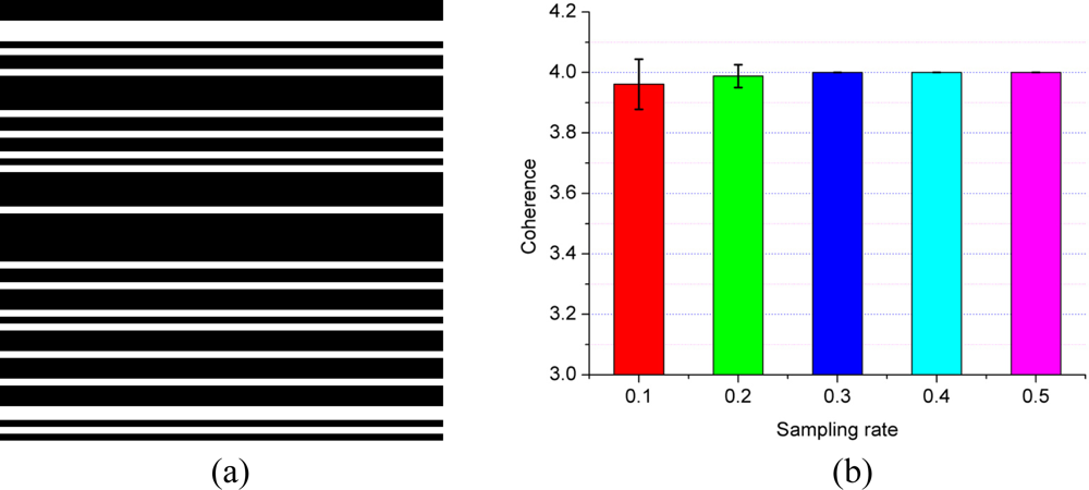
The undersampling of Θ in the indirect dimension is carried out by choosing some of the FID points in this dimension. To make this undersampling intuitive, a binary mask which has the same size of 2D FID is shown as the undersampling pattern in Figure 6(a). If the value of mask at location (i, j) is equal to 1 shown as a white pixel, the FID at location (i, j) is acquired.
To avoid the influence of randomness on the coherence calculation, Θ is randomly generated 10 times and the coherence is averaged for each sampling rate. Figure 6(b) shows that the coherence between wavelet and undersampled Fourier operator Φ is larger than the coherence between identity matrix and Φ. So, from the aspect of coherence, it is also better to choose the identity matrix for self-sparse NMR spectra.
3.4. Reconstruction of Self-Sparse NMR Spectra with ℓp Norm Minimization
In this paper, we propose to reconstruct the self-sparse 2D NMR spectra with identity matrix I as follows:
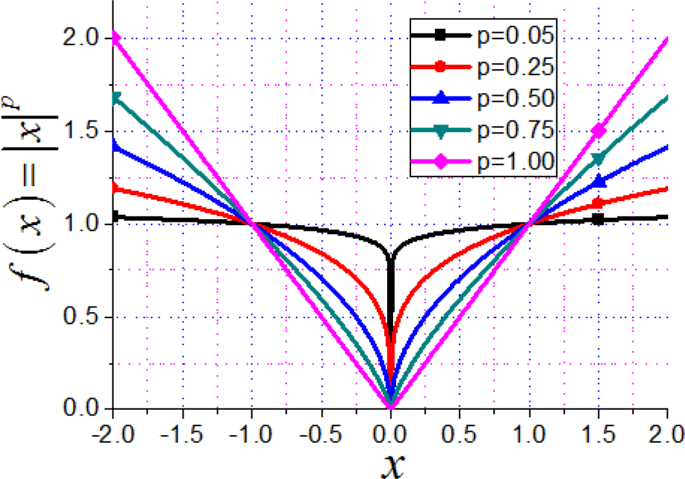
To further improve the reconstruction, a ℓp (0 < p < 1) norm is incorporated which has been demonstrated to give better reconstruction of MR images with fewer measurements than ℓ1 norm does [34–37]:
Theoretically, the required number of measurements [38] by enforcing the sparsity with a ℓp (0 < p < 1) norm is:
In this paper, the ℓp norm minimization is solved via the p-shrinkage operator [39] with continuation algorithm [40] because of its fast computation. This algorithm is abbreviated as PSOCA and summarized in Algorithm 1.

| Initialization: |
| Input the sampled FID data y, set the regularization parameter λ =108 and tolerance of inner loop η = 5 × 10⁻³. Initialize x = FΘT y, xlast = x, β = 26, and α = 0. |
| Main: |
| While β ≤ 216 |
| Inner loop: |
| 1. Given x, |
| For j = 1 to J, solve Equation (20), the solution is α; |
| 2. Given α, solve Equation (22), the solution is x; |
| 3. If ‖Δx‖ = ‖xlast – x‖ > η, xlast ← x, go to step 1; Otherwise, go to step 4; |
| Outer loop: |
| 4. x̂ ← x, β ← 2β, go to step 1. |
| End While |
| Output: x̂ |
For a given continuation parameter β, PSOCA is implemented to solve two sub-problems:
(1) p-shrinkage operator
(2) solve the linear equation:
4. Simulation Results and Analysis
In this section, we will show the advantages of the proposed method in two aspects: (1) identity matrix as the sparsifying transform is compared with wavelet transform; (2) ℓp norm minimization is compared with ℓ1 norm minimization. The recommended value of p is 0.5 for stability from empirical experiments [34]. The notation ℓ0.5 is short for ℓp with p = 0.5. The typical ℓ1 norm minimization algorithms compared in this paper include iterative soft thresholding (IST) algorithm [16,41–43], alternating and continuation algorithm (ACA) [40]. The ACA is just p = 1 in PSOCA.
Because regions of small spectrum values usually contain no peaks for practical analysis, we set magnitude smaller than a constant T to be zero according to:
Suppose x̂ denotes the reconstructed spectrum from undersampled FID, relative ℓ2 norm error (RLNE) is defined to measure the reconstruction error as:
4.1. Reconstruction of the spectra
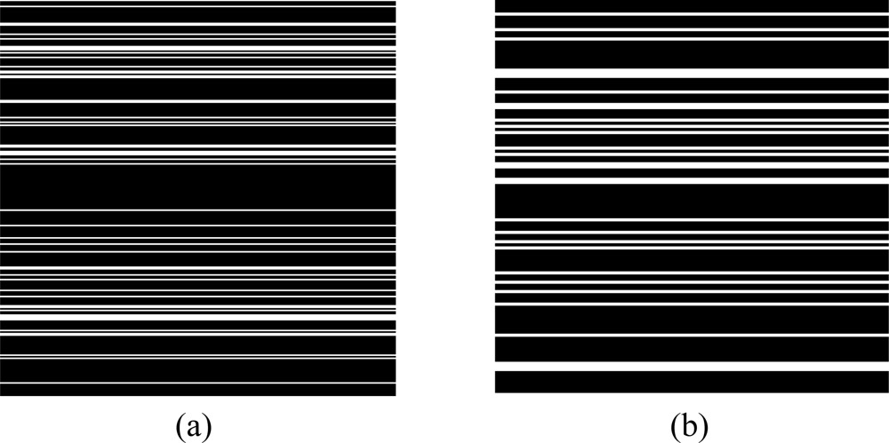
The improvement by using the proposed method is verified from the less crowed 1H-1H COSY spectrum and more crowded 1H-13C COSY spectrum. The sampling patterns of the two spectra are shown in Figure 8.
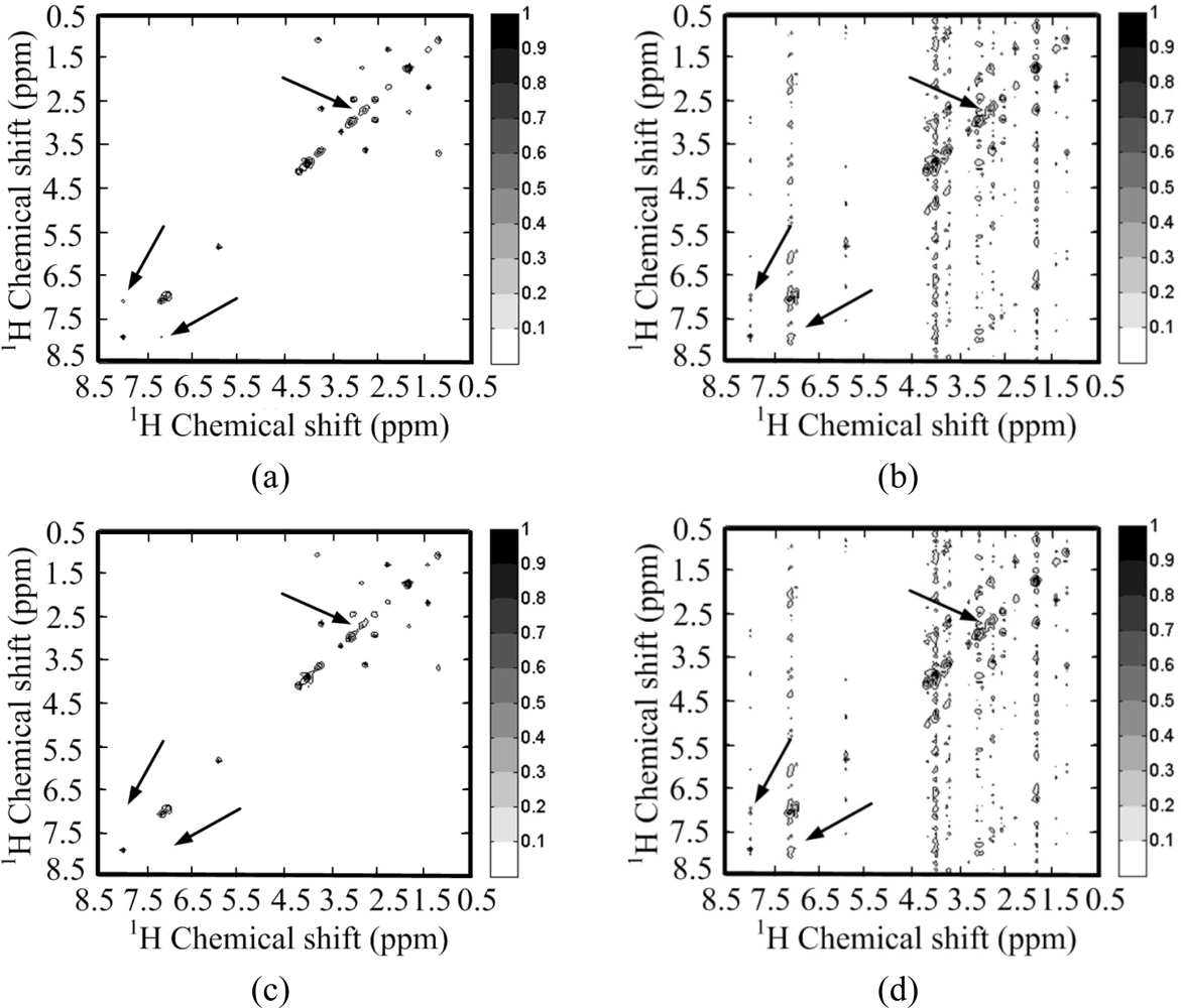
Figure 9(c–h) show the reconstructed 1H-1H COSY spectra corresponding to the sampling pattern in Figure 9(a) with a sampling rate of 0.20. With the ℓ1 norm minimization, all the peaks are recovered successfully by using identity matrix (Figure 9(d,f)), while some peaks are lost by using wavelets (Figure 9(c,e)).
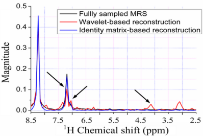
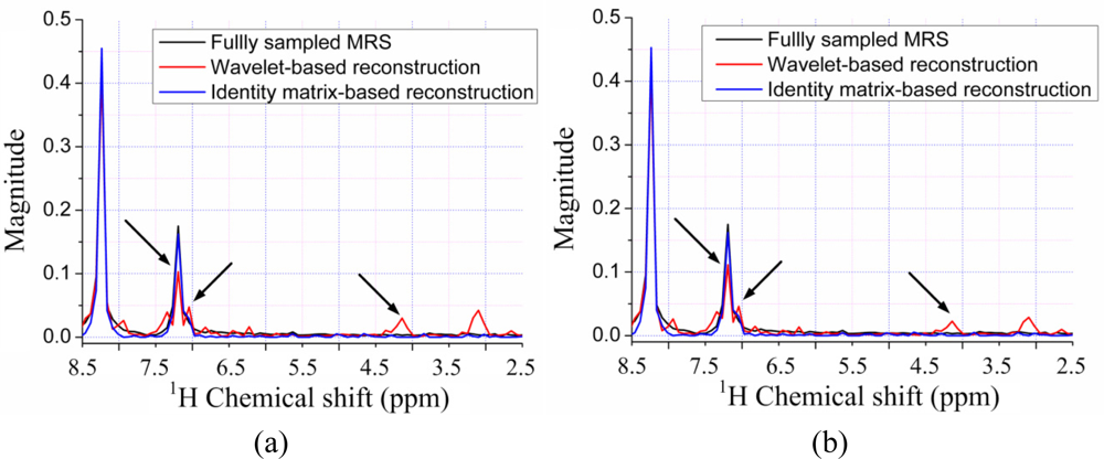
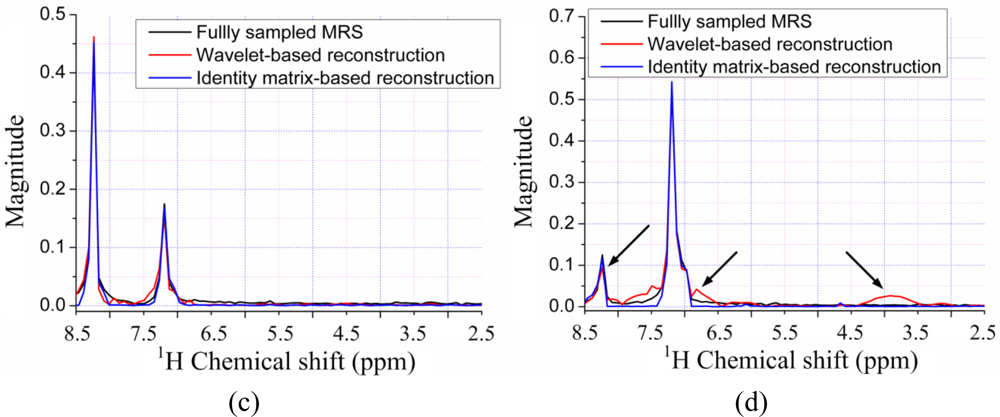
Since the contours for the marked peaks look faint, we also plot the 1D slices along the indirect dimension in Figure 10. The height of one peak in the wavelet-based reconstruction in Figure 10(a,b) are much lower than those in the fully sampled spectrum, leading to the peak lost in the contour plots in Figure 9(c,e).
Furthermore, the nonlinear operation on wavelet coefficients induces the artifacts labeled in Figure 9(c,e). This phenomenon is also observed in the 1D slices shown in Figure 10(a,b), where wavelet reconstruction generates illusive peaks. With the ℓ0.5 norm minimization, the errors caused from wavelet and identity matrix reconstruction are reduced, as shown in Table 1. One can still observe the reduced peak height and artifacts in wavelet-based reconstruction, but identity matrix performs very well (Figure 10(d)). The advantage of ℓ0.5 norm over ℓ1 norm is obvious in the crowded 1H-13C COSY spectra, as will be shown in the following discussion.
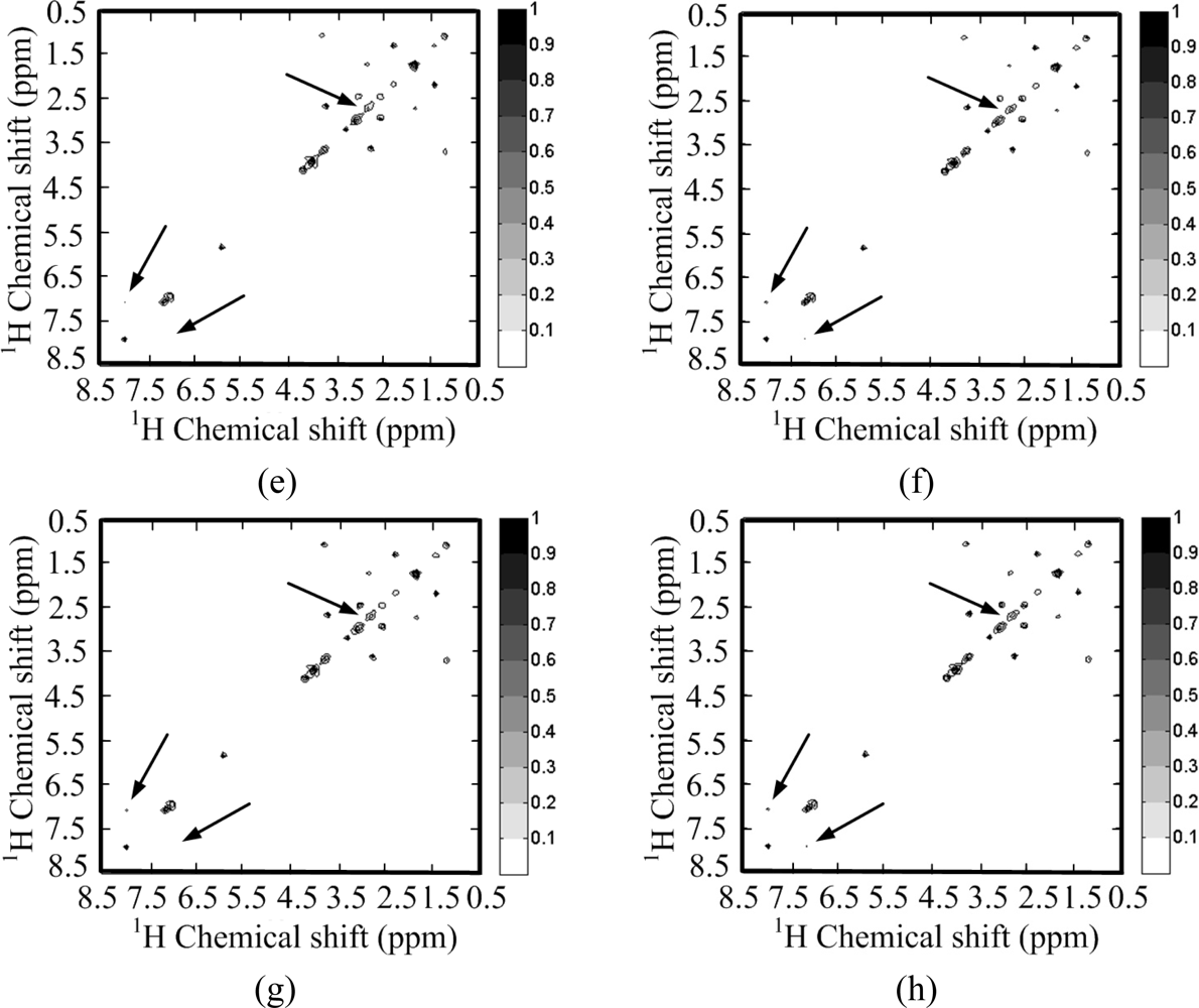
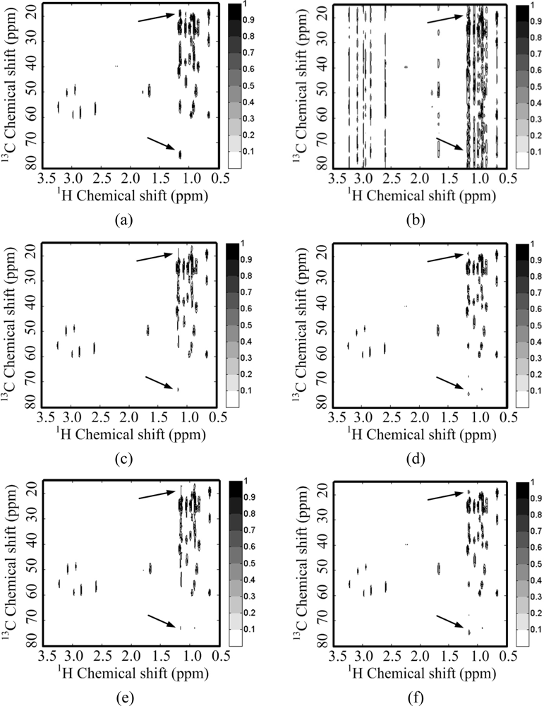
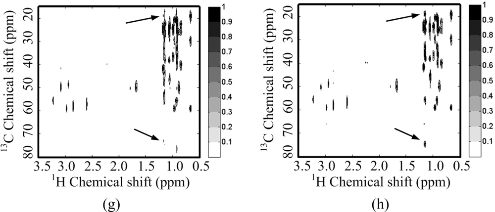
Figure 11 shows the reconstructed 1H-13C COSY spectra corresponding to the sampling pattern in Figure 8(b) with a sampling rate of 0.25. Some peaks are obviously lost in the reconstructed spectra using wavelets with both ℓ1 norm and ℓ0.5 norm minimization (Figure 11(c,e,g)). These lost peaks are found in the identity matrix-based reconstruction spectra (Figure 11(d,f,h)). With the ℓ0.5 norm minimization, the intensities of the peaks marked with arrow in Figure 11(h) are more consistent to the fully sampled spectra in Figure 11(b) than those in the reconstructed spectra with the ℓ1 norm minimization (Figure 11(d,f)). The smallest reconstruction error is achieved with the proposed identity matrix-based ℓ0.5 norm minimization method (Table 2).
All above simulation results demonstrate that wavelet-based reconstruction obviously induces the loss of some peaks in the crowded 1H-13C COSY spectrum and loss of some weak peaks in the less crowded 1H-1H COSY spectrum. The wavelet may even worsen the reconstructed spectra. Thus, it is not a good choice to use wavelets for the self-sparse spectra discussed in this paper.
4.2. Discussion on the Computation
Our simulation is run on a dual core 2.2 GHz CPU laptop with 3 GB RAM. The computational time for the algorithms using wavelet is two times that using the identity matrix, as shown in Table 3.
In the simulation, with the gradual increase of continuation parameter β, the previous solution was used as a ‘warm start’ for the next alternating optimization in the PSOCA. For a given β, with the increase of iterations in inner loop, the difference between reconstructed spectra decreases (see Figure 12(a)), so does the error between the reconstructed spectrum and the fully sampled spectrum (see Figure 12(b)). The reconstruction error decreases when β becomes large in the outer loop. The computational time of ℓ0.5 norm minimization in PSOCA is nearly four times as that of ℓ1 norm minimization, as shown in Table 3.
5. Conclusions and Future Work
Random sampling in the indirect dimension is introduced to reconstruct 2D self-sparse NMR spectra within the CS framework. Based on the assumption of sparsity of NMR spectra, one may remove the aliasing by penalizing the ℓ1 norm on the coefficients of the sparse representation of NMR spectra. Considering the sparsity and the coherence property, we demonstrate that wavelet transform may reduce the peak height and result in loss of peaks. Thus, a wavelet is not necessary and even worsens the reconstruction of self-sparse NMR spectra. With the ℓp (p = 0.5) norm minimization, the quality of reconstructed spectra can be further improved.
However, how to define the meaningless peaks depends on applications and a qualitative analysis of self-sparse NMR spectra is needed in order to satisfy the requirement of CS. By defining regularity of ideal Lorentizian peaks with aspect to typical vanishing moment wavelet basis, it is possible to give a boundary for the approximation error of Lorentizian peaks in wavelet representation. Thus, one may quantify the sparsity of spectra composed of ideal Lorentizian peaks using wavelets. Another way is to set up a database and analyze the sparsity of the meaningful peaks based on the prior knowledge of chemists. Since the peak height may be reduced in the wavelet-based reconstruction and this reduction depends on the crowd of peaks, it is expected to give a quantitative analysis on the effect of using/skipping wavelet transform by setting up a simulated spectrum or spectrum from real chemical substance, in which the crowd of peaks and the fixed relative height of peaks are pre-defined in the spectrum. Besides, based on the coherence property in CS, the analysis of the performance of different random sampling schemes, e.g., Poisson disk sampling, may lead to further reduction of sampling rate and reconstruction error. Extension of the proposed method on higher dimensional NMR spectra is worth investigating.
Acknowledgments
This work was partially supported by the NNSF of China under Grant 10974164, and the Research Fund for the Doctoral Program of Higher Education of China under Grant 200803840019. Xiaobo Qu and Di Guo would like to acknowledge the fellowship of Postgraduates’ Oversea Study Program for Building High-Level Universities from the China Scholarship Council. The authors also thank the reviewers for their thorough review and highly appreciate the comments and suggestions, which significantly contributed to improving the quality of this article.
References
- Bretthorst, GL. Nonuniform sampling: Bandwidth and aliasing. Concept Magn. Reson. A 2008, 32A, 417–435. [Google Scholar]
- Maciejewski, MW; Qui, HZ; Rujan, I; Mobli, M; Hoch, JC. Nonuniform sampling and spectral aliasing. J. Magn. Reson 2009, 199, 88–93. [Google Scholar]
- Kazimierczuk, K; Kozminski, W; Zhukov, I. Two-dimensional fourier transform of arbitrarily sampled NMR data sets. J. Magn. Reson 2006, 179, 323–328. [Google Scholar]
- Kazimierczuk, K; Zawadzka, A; Kozminski, W. Optimization of random time domain sampling in multidimensional NMR. J. Magn. Reson 2008, 192, 123–130. [Google Scholar]
- Vosegaard, T; Nielsen, NC. Defining the sampling space in multidimensional NMR experiments: What should the maximum sampling time be? J. Magn. Reson 2009, 199, 146–158. [Google Scholar]
- Mobli, M; Hoch, JC. Maximum entropy spectral reconstruction of nonuniformly sampled data. Concept Magn. Reson. A 2008, 32A, 436–448. [Google Scholar]
- Jee, JG. Real-time acquisition of three dimensional NMR spectra by non-uniform sampling and maximum entropy processing. Bull. Korean Chem. Soc 2008, 29, 2017–2022. [Google Scholar]
- Coggins, BE; Zhou, P. High resolution 4-D spectroscopy with sparse concentric shell sampling and FFT-CLEAN. J. Biomol. NMR 2008, 42, 225–239. [Google Scholar]
- Yoon, JW; Godsill, SJ. Bayesian inference for multidimensional NMR image reconstruction. Proceedings of the European Signal Processing Conference (EUSIPCO), Florence, Italy, 4–8 September 2006.
- Lin, MJ; Huang, YQ; Chen, X; Cai, SH; Chen, Z. High-resolution 2D NMR spectra in inhomogeneous fields based on intermolecular multiple-quantum coherences with efficient acquisition schemes. J. Magn. Reson 2011, 208, 87–94. [Google Scholar]
- Candes, EJ; Romberg, J; Tao, T. Robust uncertainty principles: Exact signal reconstruction from highly incomplete frequency information. IEEE Trans. Inform. Theory 2006, 52, 489–509. [Google Scholar]
- Donoho, DL. Compressed sensing. IEEE Trans. Inform. Theory 2006, 52, 1289–1306. [Google Scholar]
- Lustig, M; Donoho, D; Pauly, JM. Sparse MRI: The application of compressed sensing for rapid MR imaging. Magn. Reson. Med 2007, 58, 1182–1195. [Google Scholar]
- Duarte, MF; Davenport, MA; Takhar, D; Laska, JN; Sun, T; Kelly, KF; Baraniuk, RG. Single-pixel imaging via compressive sampling. IEEE Signal Proc. Mag 2008, 25, 83–91. [Google Scholar]
- Wright, J; Yang, AY; Ganesh, A; Sastry, SS; Ma, Y. Robust face recognition via sparse representation. IEEE Trans. Pattern Anal 2009, 31, 210–227. [Google Scholar]
- Drori, I. Fast l1 minimization by iterative thresholding for multidimensional NMR spectroscopy. EURASIP J Adv Sig Proc 2007. [Google Scholar] [CrossRef]
- Matsuki, Y; Eddy, MT; Herzfeld, J. Spectroscopy by integration of frequency and time domain information for fast acquisition of high-resolution dark spectra. J. Am. Chem. Soc 2009, 131, 4648–4656. [Google Scholar]
- Kazimierczuk, K; Orekhov, VY. Accelerated NMR spectroscopy by using compressed sensing. Angew. Chem. Int. Ed 2011, 50, 5556–5559. [Google Scholar]
- Holland, DJ; Bostock, MJ; Gladden, LF; Nietlispach, D. Fast multidimensional NMR spectroscopy using compressed sensing. Angew. Chem. Int. Ed 2011, 50, 6548–6551. [Google Scholar]
- Shrot, Y; Frydman, L. Compressed sensing and the reconstruction of ultrafast 2D NMR data: Principles and biomolecular applications. J. Magn. Reson 2011, 209, 352–358. [Google Scholar]
- Hoch, JC; Stern, AS. NMR Data Processing; Wiley-Liss: New York, NY, USA, 1996; p. 38. [Google Scholar]
- Keeler, J. Understanding NMR Spectroscopy; Wiley: New York, NY, USA, 2005; Chapter 7,; pp. 1–30. [Google Scholar]
- Aue, WP; Bartholdi, E; Ernst, RR. 2-Dimensional spectroscopy: Application to nuclear magnetic-resonance. J. Chem. Phys 1976, 64, 2229–2246. [Google Scholar]
- Ernst, RR; Bodenhausen, G; Wokaun, A. Principles of Nuclear Magnetic Resonance in One and Two dimensions; Oxford University Press: New York, NY, USA, 1990. [Google Scholar]
- Frydman, L; Scherf, T; Lupulescu, A. The acquisition of multidimensional NMR spectra within a single scan. Proc. Natl. Acad. Sci. USA 2002, 99, 15858–15862. [Google Scholar]
- De Graaf, RA. In Vivo NMR Spectroscopy Principles and Techniques, 3rd ed; John Wiley & Sons: Hoboken, NJ, USA, 2007; pp. 389–444. [Google Scholar]
- Donoho, DL; Huo, XM. Uncertainty principles and ideal atomic decomposition. IEEE Trans. Inform. Theory 2001, 47, 2845–2862. [Google Scholar]
- Candes, E; Romberg, J. Sparsity and incoherence in compressive sampling. Inverse Probl 2007, 23, 969–985. [Google Scholar]
- Candès, EJ; Romberg, J. Practical signal recovery from random projections. Proceedings of the Wavelet Applications in Signal and Image Processing XI, San Diego, CA, USA, 31 July–4 August 2005; p. 5914.
- Elad, M. Optimized projections for compressed sensing. IEEE Trans. Signal Process 2007, 55, 5695–5702. [Google Scholar]
- Hoch, JC; Maciejewski, MW; Filipovic, B. Randomization improves sparse sampling in multidimensional NMR. J. Magn. Reson 2008, 193, 317–320. [Google Scholar]
- Candes, EJ. The restricted isometry property and its implications for compressed sensing. Compt. Rendus Math 2008, 346, 589–592. [Google Scholar]
- Stern, AS; Donoho, DL; Hoch, JC. NMR data processing using iterative thresholding and minimum l1-norm reconstruction. J. Magn. Reson 2007, 188, 295–300. [Google Scholar]
- Chartrand, R. Exact reconstruction of sparse signals via nonconvex minimization. IEEE Signal Proc. Lett 2007, 14, 707–710. [Google Scholar]
- Trzasko, J; Manduca, A. Highly undersampled magnetic resonance image reconstruction via homotopic l0-minimization. IEEE Trans. Med. Imaging 2009, 28, 106–121. [Google Scholar]
- Qu, X; Cao, X; Guo, D; Hu, C; Chen, Z. Compressed sensing MRI with combined sparsifying transforms and smoothed l0 norm minimization. Proceedings of the IEEE International Conference on Acoustics, Speech and Signal Processing—ICASSP’10, Dallas, TX, USA, 14–19 March 2010; pp. 626–629.
- Majumdar, A; Ward, R. Under-determined non-cartesian MR reconstruction with non-convex sparsity promoting analysis prior. Proceedings of the Medical Image Computing and Computer-Assisted Intervention—MICCAI’10, Beijing, China, 20–24 September 2010; pp. 513–520.
- Chartrand, R; Staneva, V. Restricted isometry properties and nonconvex compressive sensing. Inverse Probl 2008, 24, 1–14. [Google Scholar]
- Chartrand, R. Fast algorithms for nonconvex compressive sensing: MRI reconstruction from very few data. Proceedings of the 2009 IEEE International Symposium on Biomedical Imaging: From Nano to Macro—ISBI’09, Boston, MA, USA, 28 June–1 July 2009; pp. 262–265.
- Yang, JF; Zhang, Y; Yin, WT. A fast alternating direction method for TV L1-L2 signal reconstruction from partial fourier data. IEEE J. Sel. Top. Signal Process 2010, 4, 288–297. [Google Scholar]
- Qu, XB; Zhang, WR; Guo, D; Cai, CB; Cai, SH; Chen, Z. Iterative thresholding compressed sensing MRI based on contourlet transform. Inverse Probl. Sci. En 2010, 18, 737–758. [Google Scholar]
- Guo, D; Qu, XB; Huang, LF; Yao, Y. Sparsity-based spatial interpolation in wireless sensor networks. Sensors 2011, 11, 2385–2407. [Google Scholar]
- Zibulevsky, M; Elad, M. L1-L2 optimization in signal and image processing. IEEE Signal Proc. Mag 2010, 27, 76–88. [Google Scholar]


| Methods | Zero-filling | IST ℓ1 | PSOCA ℓ1 | PSOCA ℓ0.5 | |
|---|---|---|---|---|---|
| Wavelet | RLNE (T = 0) | 2.054 | 0.415 | 0.393 | 0.430 |
| RLNE (T = 0.1) | 0.059 | 0.012 | 0.010 | 0.007 | |
| Identity matrix | RLNE (T = 0) | 2.054 | 0.282 | 0.273 | 0.245 |
| RLNE (T = 0.1) | 0.059 | 0.010 | 0.007 | 0.022 | |
| Methods | Zero-filling | IST ℓ1 | PSOCA ℓ1 | PSOCA ℓ0.5 | |
|---|---|---|---|---|---|
| Wavelet | RLNE (T = 0) | 1.687 | 0.547 | 0.533 | 0.541 |
| RLNE (T = 0.1) | 0.098 | 0.044 | 0.042 | 0.042 | |
| Identity matrix | RLNE (T = 0) | 1.687 | 0.422 | 0.405 | 0.343 |
| RLNE (T = 0.1) | 0.098 | 0.033 | 0.031 | 0.027 | |
| Methods | Zero-filling | IST ℓ1 | PSOCA ℓ1 | PSOCA ℓ0.5 | ||||
|---|---|---|---|---|---|---|---|---|
| 1H-1H | 1H-13C | 1H-1H | 1H-13C | 1H-1H | 1H-13C | 1H-1H | 1H-13C | |
| Wavelet | 0.1 | 0.1 | 11.1 | 56.8 | 8.5 | 70.4 | 29.1 | 221.2 |
| Identity matrix | 0.1 | 0.1 | 5.9 | 27.5 | 5.7 | 31.8 | 16.0 | 105.6 |
© 2011 by the authors; licensee MDPI, Basel, Switzerland. This article is an open access article distributed under the terms and conditions of the Creative Commons Attribution license (http://creativecommons.org/licenses/by/3.0/).
Share and Cite
Qu, X.; Guo, D.; Cao, X.; Cai, S.; Chen, Z. Reconstruction of Self-Sparse 2D NMR Spectra from Undersampled Data in the Indirect Dimension. Sensors 2011, 11, 8888-8909. https://doi.org/10.3390/s110908888
Qu X, Guo D, Cao X, Cai S, Chen Z. Reconstruction of Self-Sparse 2D NMR Spectra from Undersampled Data in the Indirect Dimension. Sensors. 2011; 11(9):8888-8909. https://doi.org/10.3390/s110908888
Chicago/Turabian StyleQu, Xiaobo, Di Guo, Xue Cao, Shuhui Cai, and Zhong Chen. 2011. "Reconstruction of Self-Sparse 2D NMR Spectra from Undersampled Data in the Indirect Dimension" Sensors 11, no. 9: 8888-8909. https://doi.org/10.3390/s110908888