<?xml version="1.0" encoding="UTF-8"?>
<!DOCTYPE article PUBLIC "-//NLM//DTD Journal Publishing DTD v2.3 20070202//EN" "journalpublishing.dtd">
<article xmlns:mml="http://www.w3.org/1998/Math/MathML" xmlns:xlink="http://www.w3.org/1999/xlink" xml:lang="en" article-type="research-article">
<front>
<journal-meta>
<journal-id journal-id-type="nlm-ta">Sensors</journal-id>
<journal-title>Sensors</journal-title>
<issn pub-type="epub">1424-8220</issn>
<publisher>
<publisher-name>Molecular Diversity Preservation International (MDPI)</publisher-name></publisher></journal-meta>
<article-meta>
<article-id pub-id-type="doi">10.3390/s110908281</article-id>
<article-id pub-id-type="publisher-id">sensors-11-08281</article-id>
<article-categories>
<subj-group>
<subject>Article</subject></subj-group></article-categories>
<title-group>
<article-title>Robust Automatic Focus Algorithm for Low Contrast Images Using a New Contrast Measure</article-title></title-group>
<contrib-group>
<contrib contrib-type="author">
<name><surname>Xu</surname><given-names>Xin</given-names></name><xref ref-type="aff" rid="af1-sensors-11-08281"><sup>1</sup></xref><xref ref-type="aff" rid="af2-sensors-11-08281"><sup>2</sup></xref></contrib>
<contrib contrib-type="author">
<name><surname>Wang</surname><given-names>Yinglin</given-names></name><xref ref-type="aff" rid="af1-sensors-11-08281"><sup>1</sup></xref></contrib>
<contrib contrib-type="author">
<name><surname>Tang</surname><given-names>Jinshan</given-names></name><xref ref-type="aff" rid="af2-sensors-11-08281"><sup>2</sup></xref><xref ref-type="corresp" rid="c1-sensors-11-08281"><sup>*</sup></xref></contrib>
<contrib contrib-type="author">
<name><surname>Zhang</surname><given-names>Xiaolong</given-names></name><xref ref-type="aff" rid="af2-sensors-11-08281"><sup>2</sup></xref></contrib>
<contrib contrib-type="author">
<name><surname>Liu</surname><given-names>Xiaoming</given-names></name><xref ref-type="aff" rid="af2-sensors-11-08281"><sup>2</sup></xref></contrib></contrib-group>
<aff id="af1-sensors-11-08281">
<label>1</label> Department of Computer Science and Engineering, Shanghai Jiao Tong University, NO. 800 Dongchuan Road, Shanghai 200240, China; E-Mails: <email>xuxin0336@gmail.com</email> (X.X.); <email>wang-yl@cs.sjtu.edu.cn</email> (Y.W.)</aff>
<aff id="af2-sensors-11-08281">
<label>2</label> School of Computer Science and Technology, Wuhan University of Science and Technology, NO. 947 Heping Road, Wuhan 430081, Hubei, China; E-Mail: <email>xiaolong.zhang@wust.edu.cn</email> (X.Z.); <email>liuxiaoming@wust.edu.cn</email> (X.L.)</aff>
<author-notes>
<corresp id="c1-sensors-11-08281">
<label>*</label>Author to whom correspondence should be addressed; E-Mail: <email>dadaotang@yahoo.com</email>; Tel.: +86-21-3420-5978; Fax: +86-21-3420-4486.</corresp></author-notes>
<pub-date pub-type="collection">
<year>2011</year></pub-date>
<pub-date pub-type="epub">
<day>25</day>
<month>8</month>
<year>2011</year></pub-date>
<volume>11</volume>
<issue>9</issue>
<fpage>8281</fpage>
<lpage>8294</lpage>
<history>
<date date-type="received">
<day>1</day>
<month>8</month>
<year>2011</year></date>
<date date-type="rev-recd">
<day>23</day>
<month>8</month>
<year>2011</year></date>
<date date-type="accepted">
<day>24</day>
<month>8</month>
<year>2011</year></date></history>
<permissions>
<copyright-statement>© 2011 by the authors; licensee MDPI, Basel, Switzerland.</copyright-statement>
<copyright-year>2011</copyright-year>
<license>
<p>This article is an open access article distributed under the terms and conditions of the Creative Commons Attribution license (http://creativecommons.org/licenses/by/3.0/).</p></license></permissions>
<abstract>
<p>Low contrast images, suffering from a lack of sharpness, are easily influenced by noise. As a result, many local false peaks may be generated in contrast measurements, making it difficult for the camera’s passive auto-focus system to perform its function of locating the focused peak. In this paper, a new passive auto-focus algorithm is proposed to address this problem. First, a noise reduction preprocessing is introduced to make our algorithm robust to both additive noise and multiplicative noise. Then, a new contrast measure is presented to bring in local false peaks, ensuring the presence of a well defined focused peak. In order to gauge the performance of our algorithm, a modified peak search algorithm is used in the experiments. The experimental results from an actual digital camera validate the effectiveness of our proposed algorithm.</p></abstract>
<kwd-group>
<kwd>auto-focus</kwd>
<kwd>low contrast</kwd>
<kwd>contrast measure</kwd>
<kwd>noise reduction</kwd></kwd-group></article-meta></front>
<body>
<sec sec-type="intro">
<label>1.</label>
<title>Introduction</title>
<p>With the rapid development of digital image processing techniques, the design of a consumer-level digital camera is inclined to introduce user-friendly cameras which aim to provide easy way to obtain high quality imaging with minimal user intervention in tasks such as auto-focus (AF). The basic idea of AF is to replace the tedious process of manual focusing with automatic adjustment of the lens of the camera to the right position, ensuring the image is well positioned at the focal plane [<xref ref-type="bibr" rid="b1-sensors-11-08281">1</xref>]. AF is a key factor affecting the sharpness of a final captured image. It is based on the fact that an object in the image appears the sharpest when it is in focus. Otherwise, image will be blurry in an out of focus position [<xref ref-type="bibr" rid="b2-sensors-11-08281">2</xref>]. Thus, the most high quality imaging is obtained in large part by how the lens is adjusted by camera’s AF system to bring an image into focus where sharpness is maximized [<xref ref-type="bibr" rid="b3-sensors-11-08281">3</xref>].</p>
<p>Many AF systems were developed in the past, which can be classified into two types of systems: active AF and passive AF [<xref ref-type="bibr" rid="b4-sensors-11-08281">4</xref>]. Active AF can be achieved through the use of external sensors or measurement tools. The advantage of active AF lies in its ability to focus under different lighting conditions, particular in a low-level luminance environment. However, due to the high infrared or ultrasound reflectivity of external sensor or measurement tool, they may encounter difficulty when focusing through window or glass [<xref ref-type="bibr" rid="b5-sensors-11-08281">5</xref>]. In addition, it is generally costly to calculate the distance between the lens and the object of interest. On the contrary, the calculation of in-focus position in passive AF relies on the image information only, and we do not need to consider the reflectivity in passive AF, because no external sensor is used. As a result, most consumer-level digital cameras deploy passive AF.</p>
<p>
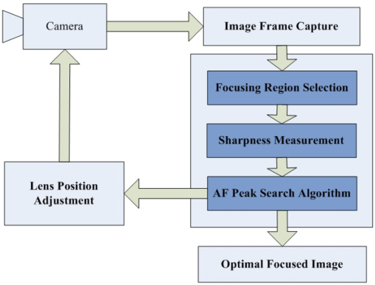
A passive AF system generally includes three components: focusing region selection, sharpness measurement, and peak search [<xref ref-type="bibr" rid="b4-sensors-11-08281">4</xref>]. As illustrated in <xref ref-type="fig" rid="f1-sensors-11-08281">Figure 1</xref>, a passive AF system normally operates in an iterative manner. First, an image is captured by the camera at the current lens position or focal length. Next, the focusing region selection procedure determines which part of the captured image is used for sharpness computation. Then, a sharpness measurement is applied to that focusing region to calculate a fitness value. Finally, a peak search step is performed to obtain the maximum sharpness or best lens position from the fitness value candidates.</p>
<p>Unfortunately, most passive AF systems do not always work well for low contrast images obtained under dim lighting conditions. Passive AF extracts a measure of sharpness from the image itself, and treats a defocused image as the image generated by convolving a focused image with a low-pass filter whose bandwidth is proportional to the degree of focus [<xref ref-type="bibr" rid="b6-sensors-11-08281">6</xref>]. The less an image is focused, the more details it loses. Thus, passive AF usually is based on the high frequency content of the image computed from focus windows, assigning more weight to the high frequency content when evaluating the degree of focus [<xref ref-type="bibr" rid="b7-sensors-11-08281">7</xref>]. However, under low light conditions, there is little content in the high frequency range, making it difficult to extract adequate sharpness information. The improvement of low-light AF performance is important for capturing high-quality images to meet consumers’ demand in undesired lighting conditions. The goal of our work described in this paper is to overcome this weakness for most passive AF systems, and propose a robust algorithm which is capable of handling low contrast images in noisy environments.</p></sec>
<sec>
<label>2.</label>
<title>Related Works</title>
<p>
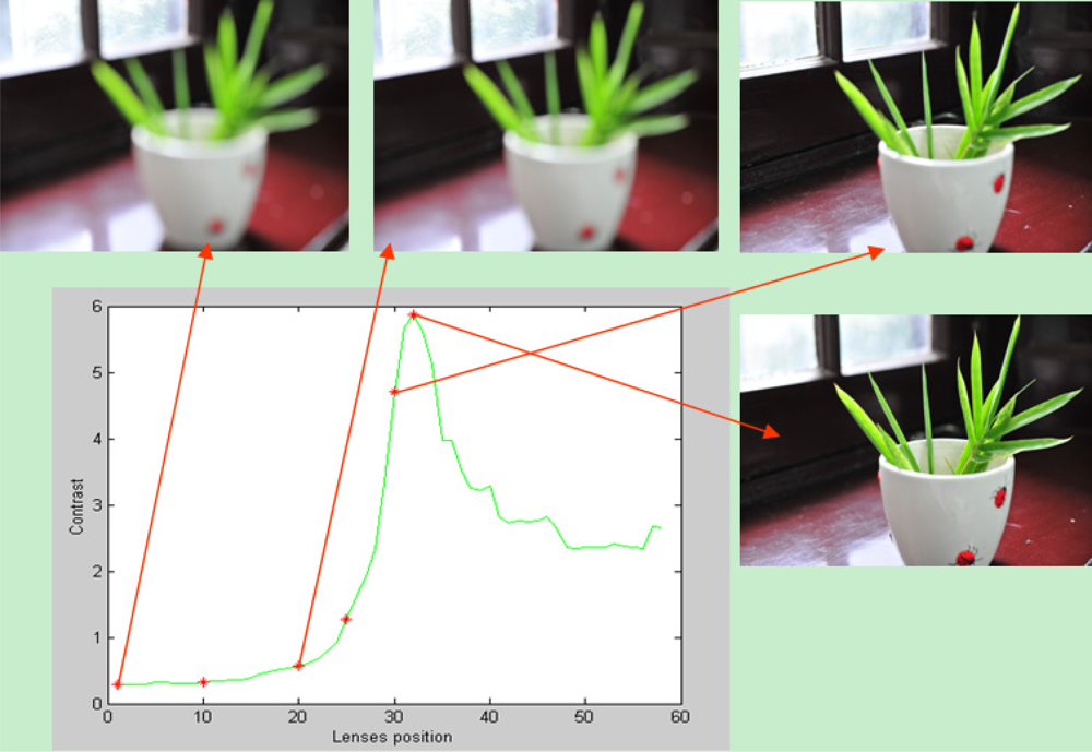
Sharpness function is a quantitative description of the image sharpness in mathematics, and it is a numerical measure that provides a value indicating the degree of focus for an out-of-focus image [<xref ref-type="bibr" rid="b5-sensors-11-08281">5</xref>,<xref ref-type="bibr" rid="b8-sensors-11-08281">8</xref>]. Because the sharpness is related to the contrast of an image and thus we can use contrast measure as the sharpness function. As illustrated in <xref ref-type="fig" rid="f2-sensors-11-08281">Figure 2</xref>, the change of contrast accompanies the change of lens position. The contrast reaches a maximum for the best focused image and decreases as the image blurs.</p>
<p>Many contrast measures have been used for passive AF. In [<xref ref-type="bibr" rid="b4-sensors-11-08281">4</xref>], comparison of different AF algorithms is made to explore their relative merits through examining them in a variety of scenes. Results indicate that 2D spatial measurement methods such as Tenengrad [<xref ref-type="bibr" rid="b9-sensors-11-08281">9</xref>,<xref ref-type="bibr" rid="b10-sensors-11-08281">10</xref>], Prewitt Edge detection [<xref ref-type="bibr" rid="b11-sensors-11-08281">11</xref>], and Laplacian [<xref ref-type="bibr" rid="b6-sensors-11-08281">6</xref>] yield best performance in terms of accuracy and unimodality. However, they are very sensitive to noise, and not robust to different scene conditions such as low light conditions.</p>
<p>On the contrary, variance based methods are fast and robust. The basic idea is to calculate the variance of image intensity. The image is best focused when the variance reaches a maximum [<xref ref-type="bibr" rid="b6-sensors-11-08281">6</xref>]. A typical method in discrete cosine transform (DCT) domain is to compute the AC coefficients of images, which can also be used to represent information about variance function of the luminance [<xref ref-type="bibr" rid="b12-sensors-11-08281">12</xref>]. However, low light conditions pose a major problem for traditional variance based methods due to its poor discrimination power. In low light conditions, contrast measures become fluctuant, and non-uniformity in image intensity seems to be not distinct when the focus changes. As a result, it is quite difficult to locate the peak.</p>
<p>Recently, several modified variance based methods have been presented for low contrast images. Shen <italic>et al</italic>. [<xref ref-type="bibr" rid="b13-sensors-11-08281">13</xref>] scaled the AC coefficients by the overall intensity of image. They calculated both AC coefficients and DC coefficients of image. Then the ratio between AC coefficients and DC coefficients was defined as a contrast measure. The purpose of this method is to compensate and give rise to a homologous region. As a result, this method can work well both for ordinary images as well as low contrast images. Lee <italic>et al</italic>. [<xref ref-type="bibr" rid="b14-sensors-11-08281">14</xref>] further improved Shen’s method, which can avoid the iterative moving of step motor. The nonlinear regression routine is used to quickly predict the location of the maximum focus value through a Gaussian profile fitting. Afterwards, Kristan <italic>et al</italic>. [<xref ref-type="bibr" rid="b15-sensors-11-08281">15</xref>] proposed a focus measure based on the Bayes spectral entropy of the image spectrum. DCT was used to map between the spatial and spectral domains. The image was divided into non-overlapping sub-images of 8 × 8 pixels, where sharpness values are calculated separately. The mean of the sharpness values is taken as a measure of overall focus. However, this measure needs to establish some predefined threshold, which varies with the content of an image. Lee <italic>et al</italic>. [<xref ref-type="bibr" rid="b16-sensors-11-08281">16</xref>] used the ratio of the AC and DC components in DCT as the measure of focus. The lowest five AC components and a DC component coefficient were selected, which contained the most energy (information) of an image as well as the detailed edge and base edge information.</p>
<p>However, due to the neglect of existing correlations among adjacent blocks pixels in DCT computation, it may incur an undesired effect called “blocking artifact” [<xref ref-type="bibr" rid="b17-sensors-11-08281">17</xref>]. In addition, the DCT-based methods require much computation time as a lot of processing is involved in conversion to and from the DCT coefficients. Aiming to address this problem, Lin [<xref ref-type="bibr" rid="b18-sensors-11-08281">18</xref>] proposed to use regional monotones of focus value variation to attenuate the influence of noise generated false peaks. The inconsistency in the motion direction of lens caused by image disturbances can be checked and corrected using these monotonous properties. However, low illumination could induce a problem of low signal-to-noise (S/N) ratio for focus value measure, which makes it difficult to obtain the monotonous properties because of the noise influence. Afterwards, Gamadia <italic>et al</italic>. [<xref ref-type="bibr" rid="b3-sensors-11-08281">3</xref>] processed low contrast images in a different way. They attempted to reduce the effect of the additive white Gaussian noise through introducing image enhancement preprocessing steps. This method is computationally simple, and can improve low light AF performance. However, the discrimination power of their proposed contrast measure is not robust. For a raw image corrupted by another kind of noise except for the additive white Gaussian noise, multiplicative noise for example, their method may fail to work well.</p>
<p>Besides enhancing image contrast, other methods for enabling passive AF in low light conditions include increasing the light intensity via external assist or flash lights [<xref ref-type="bibr" rid="b19-sensors-11-08281">19</xref>], increasing the exposure time [<xref ref-type="bibr" rid="b20-sensors-11-08281">20</xref>], and increasing the size of the focus window. Unfortunately, these methods all fail to be implemented in consumer-level digital cameras due to different limitations. Although the use of light emitting diodes (LEDs) as an AF assist in digital cameras is a standard feature, their use is not always allowed in some locations such as cinemas and museums [<xref ref-type="bibr" rid="b21-sensors-11-08281">21</xref>]. Moreover, the use of external lights may cause a distraction from the moment of a candid shot and result in the degradation of image quality [<xref ref-type="bibr" rid="b3-sensors-11-08281">3</xref>]. The increasing of exposure time contributes to the increasing of sensor integration time, and thus enhances the signal to noise ratios (SNR). However, longer sensor integration time may cause the effect of lowering the capture frame rate, and result in undesired motion blur [<xref ref-type="bibr" rid="b20-sensors-11-08281">20</xref>]. The increasing of focus window size accompanied the increasing of computation time in contrast measure computation. This may lead to an increase in AF lag time [<xref ref-type="bibr" rid="b7-sensors-11-08281">7</xref>].</p>
<p>In this paper, we propose a new passive AF algorithm which is capable of handling low contrast images in noisy environments. A denoising preprocessing is first introduced to reduce the effect of both additive noise and multiplicative noise. Aiming to reduce the difficulty of peak search, a new variance based contrast measure is presented which can further enhance the low contrast image. This contrast measure can carry more information about the image discontinuities, and thus has more discrimination power. Finally, a modified hill climbing algorithm is used to find the focused lens position. Our method was tested on a number of low contrast image sequences captured by an actual digital camera, and result indicates that this algorithm provides an effective means of improving AF performance for low contrast image in noisy conditions. The remainder of this paper is organized as follows. Section 3 proposes a new passive AF algorithm and provides a theoretical analysis of its effectiveness. Experimental results obtained from several image sequences are presented in Section 4. The conclusions are given in Section 5.</p></sec>
<sec>
<label>3.</label>
<title>Proposed Passive AF Algorithm</title>
<p>Like the traditional passive AF system illustrated in <xref ref-type="fig" rid="f1-sensors-11-08281">Figure 1</xref>, our proposed AF algorithm also includes three components: focusing region selection, contrast measurement, and peak search. Differently, before proceeding to these components, a noise reduction preprocessing using the modified bilateral filter is introduced to make our algorithm robust to different types of noise. In our study, the region of interest is not restricted to a specific area of the image. Thus we select the entire scene of the image as the focusing region. Then, in order to improve the performance of our AF algorithm under low light conditions, we propose a new contrast measurement which can make the curve peak be easily distinguished from local false peaks generated by noise. Finally, the modified peak search algorithm is presented to gauge the improvement in performance.</p>
<sec>
<label>3.1.</label>
<title>Noise Reduction Preprocessing</title>
<p>As stated previously, most of current noise reduction preprocessing for low contrast image is performed under the assumption of an additive noise model, for example, additive white Gaussian noise [<xref ref-type="bibr" rid="b3-sensors-11-08281">3</xref>,<xref ref-type="bibr" rid="b13-sensors-11-08281">13</xref>]. In our previous work [<xref ref-type="bibr" rid="b22-sensors-11-08281">22</xref>], additive noise was removed by a Wiener filter, which is the optimal linear filter for removing additive noise in the mean square error sense [<xref ref-type="bibr" rid="b23-sensors-11-08281">23</xref>,<xref ref-type="bibr" rid="b24-sensors-11-08281">24</xref>]. However, it is computationally complex, requiring the use of large memory resources due to its 2D Fast Fourier Transform operations. Thus, it is not suitable for deployment in consumer level digital cameras due to their limited cost and size requirements. An alternative to the Wiener filter would be to use a bilateral filter. The basic idea of the bilateral filter is to replace a pixel value in an image by a weighted mean of its neighbors, and the weights depend on both the spatial distance and the intensity distance [<xref ref-type="bibr" rid="b25-sensors-11-08281">25</xref>,<xref ref-type="bibr" rid="b26-sensors-11-08281">26</xref>]. The bilateral filter is a good choice for removing additive noise because it is stable and simple [<xref ref-type="bibr" rid="b27-sensors-11-08281">27</xref>].</p>
<p>According to [<xref ref-type="bibr" rid="b28-sensors-11-08281">28</xref>,<xref ref-type="bibr" rid="b29-sensors-11-08281">29</xref>], some noise, for example speckle noise, cannot be modeled as additive noise. This kind of noise, modeled as multiplicative noise, is caused by the interaction between the ultrasound waves and the scatterers within the tissue [<xref ref-type="bibr" rid="b30-sensors-11-08281">30</xref>]. As we stated previously in [<xref ref-type="bibr" rid="b31-sensors-11-08281">31</xref>], in additive noise model, the difference between any two pixels from the same homogenous region is only related to the difference of the noise. Differently, in multiplicative noise, the difference between two pixels in the same homogenous region not only depends on the difference of the noise, but also depends on the intensity of the region. As a result, the image corrupted by multiplicative noise has different distributions in different homogenous regions. Traditional bilateral filters fail to handle this granular structure. In order to cope with multiplicative noise model, we use the modified bilateral filter proposed in [<xref ref-type="bibr" rid="b31-sensors-11-08281">31</xref>], which can be described as follows:
<disp-formula id="FD1">
<label>(1)</label>
<mml:math display="block">
<mml:mrow>
<mml:mover accent="true">
<mml:mi>J</mml:mi>
<mml:mo>¯</mml:mo></mml:mover>
<mml:mrow>
<mml:mo>(</mml:mo>
<mml:mi>X</mml:mi>
<mml:mo>)</mml:mo></mml:mrow>
<mml:mo>=</mml:mo>
<mml:mfrac>
<mml:mn>1</mml:mn>
<mml:mi>C</mml:mi></mml:mfrac>
<mml:munder>
<mml:mo>∑</mml:mo>
<mml:mrow>
<mml:mi>Y</mml:mi>
<mml:mo>∈</mml:mo>
<mml:mi>N</mml:mi>
<mml:mrow>
<mml:mo>(</mml:mo>
<mml:mi>X</mml:mi>
<mml:mo>)</mml:mo></mml:mrow></mml:mrow></mml:munder>
<mml:msup>
<mml:mrow>
<mml:mi>e</mml:mi></mml:mrow>
<mml:mrow>
<mml:mfrac>
<mml:mrow>
<mml:mo>−</mml:mo>
<mml:msup>
<mml:mrow>
<mml:mrow>
<mml:mrow>
<mml:mo>‖</mml:mo>
<mml:mrow>
<mml:mi>Y</mml:mi>
<mml:mo>−</mml:mo>
<mml:mi>X</mml:mi></mml:mrow>
<mml:mo>‖</mml:mo></mml:mrow></mml:mrow></mml:mrow>
<mml:mn>2</mml:mn></mml:msup></mml:mrow>
<mml:mrow>
<mml:mn>2</mml:mn>
<mml:msubsup>
<mml:mrow>
<mml:mi>σ</mml:mi></mml:mrow>
<mml:mi>d</mml:mi>
<mml:mn>2</mml:mn></mml:msubsup></mml:mrow></mml:mfrac></mml:mrow></mml:msup>
<mml:msup>
<mml:mrow>
<mml:mi>e</mml:mi></mml:mrow>
<mml:mrow>
<mml:mfrac>
<mml:mrow>
<mml:mo>−</mml:mo>
<mml:msup>
<mml:mrow>
<mml:mrow>
<mml:mrow>
<mml:mo>‖</mml:mo>
<mml:mrow>
<mml:mi>J</mml:mi>
<mml:mrow>
<mml:mo>(</mml:mo>
<mml:mi>Y</mml:mi>
<mml:mo>)</mml:mo></mml:mrow>
<mml:mo>−</mml:mo>
<mml:mi>J</mml:mi>
<mml:mrow>
<mml:mo>(</mml:mo>
<mml:mi>X</mml:mi>
<mml:mo>)</mml:mo></mml:mrow></mml:mrow>
<mml:mo>‖</mml:mo></mml:mrow></mml:mrow></mml:mrow>
<mml:mn>2</mml:mn></mml:msup></mml:mrow>
<mml:mrow>
<mml:mn>2</mml:mn>
<mml:msubsup>
<mml:mrow>
<mml:mi>σ</mml:mi></mml:mrow>
<mml:mi>r</mml:mi>
<mml:mn>2</mml:mn></mml:msubsup>
<mml:msup>
<mml:mrow>
<mml:mrow>
<mml:mrow>
<mml:mo>‖</mml:mo>
<mml:mrow>
<mml:mi>J</mml:mi>
<mml:mrow>
<mml:mo>(</mml:mo>
<mml:mi>X</mml:mi>
<mml:mo>)</mml:mo></mml:mrow></mml:mrow>
<mml:mo>‖</mml:mo></mml:mrow></mml:mrow></mml:mrow>
<mml:mn>2</mml:mn></mml:msup></mml:mrow></mml:mfrac></mml:mrow></mml:msup>
<mml:mi>J</mml:mi>
<mml:mrow>
<mml:mo>(</mml:mo>
<mml:mi>Y</mml:mi>
<mml:mo>)</mml:mo></mml:mrow></mml:mrow></mml:math></disp-formula>where <italic>J̄</italic>(<italic>X</italic>) is the output value of a pixel, <italic>J</italic>(<italic>Y</italic>) is the input values of a pixel, <italic>N</italic>(<italic>X</italic>) is the set of spatial neighborhoods of pixel <italic>X</italic>, 
<inline-formula>
<mml:math>
<mml:mrow>
<mml:msubsup>
<mml:mrow>
<mml:mi>σ</mml:mi></mml:mrow>
<mml:mi>d</mml:mi>
<mml:mn>2</mml:mn></mml:msubsup></mml:mrow></mml:math></inline-formula> and 
<inline-formula>
<mml:math>
<mml:mrow>
<mml:msubsup>
<mml:mrow>
<mml:mi>σ</mml:mi></mml:mrow>
<mml:mi>r</mml:mi>
<mml:mn>2</mml:mn></mml:msubsup></mml:mrow></mml:math></inline-formula> are the parameters controlling the fall-off of weights in spatial and intensity domains, respectively, ‖ ‖ is Euclidean distance, C is used for the normalization and is defined as [<xref ref-type="bibr" rid="b27-sensors-11-08281">27</xref>]:
<disp-formula id="FD2">
<label>(2)</label>
<mml:math display="block">
<mml:mrow>
<mml:mi>C</mml:mi>
<mml:mo>=</mml:mo>
<mml:munder>
<mml:mo>∑</mml:mo>
<mml:mrow>
<mml:mi>Y</mml:mi>
<mml:mo>∈</mml:mo>
<mml:mi>N</mml:mi>
<mml:mrow>
<mml:mo>(</mml:mo>
<mml:mi>X</mml:mi>
<mml:mo>)</mml:mo></mml:mrow></mml:mrow></mml:munder>
<mml:msup>
<mml:mrow>
<mml:mi>e</mml:mi></mml:mrow>
<mml:mrow>
<mml:mfrac>
<mml:mrow>
<mml:mo>−</mml:mo>
<mml:msup>
<mml:mrow>
<mml:mrow>
<mml:mrow>
<mml:mo>‖</mml:mo>
<mml:mrow>
<mml:mi>Y</mml:mi>
<mml:mo>−</mml:mo>
<mml:mi>X</mml:mi></mml:mrow>
<mml:mo>‖</mml:mo></mml:mrow></mml:mrow></mml:mrow>
<mml:mn>2</mml:mn></mml:msup></mml:mrow>
<mml:mrow>
<mml:mn>2</mml:mn>
<mml:msubsup>
<mml:mrow>
<mml:mi>σ</mml:mi></mml:mrow>
<mml:mi>d</mml:mi>
<mml:mn>2</mml:mn></mml:msubsup></mml:mrow></mml:mfrac></mml:mrow></mml:msup>
<mml:msup>
<mml:mrow>
<mml:mi>e</mml:mi></mml:mrow>
<mml:mrow>
<mml:mfrac>
<mml:mrow>
<mml:mo>−</mml:mo>
<mml:msup>
<mml:mrow>
<mml:mrow>
<mml:mrow>
<mml:mo>‖</mml:mo>
<mml:mrow>
<mml:mi>J</mml:mi>
<mml:mrow>
<mml:mo>(</mml:mo>
<mml:mi>Y</mml:mi>
<mml:mo>)</mml:mo></mml:mrow>
<mml:mo>−</mml:mo>
<mml:mi>J</mml:mi>
<mml:mrow>
<mml:mo>(</mml:mo>
<mml:mi>X</mml:mi>
<mml:mo>)</mml:mo></mml:mrow></mml:mrow>
<mml:mo>‖</mml:mo></mml:mrow></mml:mrow></mml:mrow>
<mml:mn>2</mml:mn></mml:msup></mml:mrow>
<mml:mrow>
<mml:mn>2</mml:mn>
<mml:msubsup>
<mml:mrow>
<mml:mi>σ</mml:mi></mml:mrow>
<mml:mi>r</mml:mi>
<mml:mn>2</mml:mn></mml:msubsup></mml:mrow></mml:mfrac></mml:mrow></mml:msup></mml:mrow></mml:math></disp-formula></p></sec>
<sec>
<label>3.2.</label>
<title>Contrast Measure</title>
<p>A good contrast measurement should have enough discrimination ability over image sequence. As mentioned previously, various contrast measurements have been introduced and investigated in passive AF systems. The Contrast Measure based on Squared Laplacian (CMSL) yields good performance in terms of accuracy and unimodality [<xref ref-type="bibr" rid="b4-sensors-11-08281">4</xref>,<xref ref-type="bibr" rid="b6-sensors-11-08281">6</xref>,<xref ref-type="bibr" rid="b11-sensors-11-08281">11</xref>]. It can be given as follows:
<disp-formula id="FD3">
<label>(3)</label>
<mml:math display="block">
<mml:mrow>
<mml:mi>L</mml:mi>
<mml:mrow>
<mml:mo>(</mml:mo>
<mml:mrow>
<mml:mi>x</mml:mi>
<mml:mrow>
<mml:mo>,</mml:mo></mml:mrow>
<mml:mi>y</mml:mi></mml:mrow>
<mml:mo>)</mml:mo></mml:mrow>
<mml:mo>=</mml:mo>
<mml:mfrac>
<mml:mn>1</mml:mn>
<mml:mrow>
<mml:mi>J</mml:mi>
<mml:mo>*</mml:mo>
<mml:mi>K</mml:mi></mml:mrow></mml:mfrac>
<mml:munderover>
<mml:mo>∑</mml:mo>
<mml:mrow>
<mml:mi>x</mml:mi>
<mml:mo>=</mml:mo>
<mml:mn>1</mml:mn></mml:mrow>
<mml:mi>J</mml:mi></mml:munderover>
<mml:mrow>
<mml:munderover>
<mml:mo>∑</mml:mo>
<mml:mrow>
<mml:mi>y</mml:mi>
<mml:mo>=</mml:mo>
<mml:mn>1</mml:mn></mml:mrow>
<mml:mi>K</mml:mi></mml:munderover>
<mml:mrow>
<mml:mi>G</mml:mi>
<mml:msup>
<mml:mrow>
<mml:mrow>
<mml:mrow>
<mml:mo>(</mml:mo>
<mml:mrow>
<mml:mi>x</mml:mi>
<mml:mo>,</mml:mo>
<mml:mi>y</mml:mi></mml:mrow>
<mml:mo>)</mml:mo></mml:mrow></mml:mrow></mml:mrow>
<mml:mn>2</mml:mn></mml:msup></mml:mrow></mml:mrow></mml:mrow></mml:math></disp-formula>where <italic>G</italic>(<italic>x</italic>, <italic>y</italic>) is computed by:
<disp-formula id="FD4">
<label>(4)</label>
<mml:math display="block">
<mml:mrow>
<mml:mi>G</mml:mi>
<mml:mrow>
<mml:mo>(</mml:mo>
<mml:mrow>
<mml:mi>x</mml:mi>
<mml:mrow>
<mml:mo>,</mml:mo>
<mml:mtext> y</mml:mtext></mml:mrow></mml:mrow>
<mml:mo>)</mml:mo></mml:mrow>
<mml:mo>=</mml:mo>
<mml:munderover>
<mml:mo>∑</mml:mo>
<mml:mrow>
<mml:mi>i</mml:mi>
<mml:mo>=</mml:mo>
<mml:mi>x</mml:mi>
<mml:mo>−</mml:mo>
<mml:mn>1</mml:mn></mml:mrow>
<mml:mrow>
<mml:mi>x</mml:mi>
<mml:mo>+</mml:mo>
<mml:mn>1</mml:mn></mml:mrow></mml:munderover>
<mml:mrow>
<mml:mrow>
<mml:mo>|</mml:mo>
<mml:mrow>
<mml:mi>I</mml:mi>
<mml:mrow>
<mml:mo>(</mml:mo>
<mml:mrow>
<mml:mi>x</mml:mi>
<mml:mo>,</mml:mo>
<mml:mi>y</mml:mi></mml:mrow>
<mml:mo>)</mml:mo></mml:mrow>
<mml:mo>−</mml:mo>
<mml:mi>I</mml:mi>
<mml:mrow>
<mml:mo>(</mml:mo>
<mml:mrow>
<mml:mi>i</mml:mi>
<mml:mo>,</mml:mo>
<mml:mi>y</mml:mi></mml:mrow>
<mml:mo>)</mml:mo></mml:mrow></mml:mrow>
<mml:mo>|</mml:mo></mml:mrow>
<mml:mo>+</mml:mo>
<mml:munderover>
<mml:mo>∑</mml:mo>
<mml:mrow>
<mml:mi>j</mml:mi>
<mml:mo>=</mml:mo>
<mml:mi>y</mml:mi>
<mml:mo>−</mml:mo>
<mml:mn>1</mml:mn></mml:mrow>
<mml:mrow>
<mml:mi>y</mml:mi>
<mml:mo>+</mml:mo>
<mml:mn>1</mml:mn></mml:mrow></mml:munderover>
<mml:mrow>
<mml:mrow>
<mml:mo>|</mml:mo>
<mml:mrow>
<mml:mi>I</mml:mi>
<mml:mrow>
<mml:mo>(</mml:mo>
<mml:mrow>
<mml:mi>x</mml:mi>
<mml:mo>,</mml:mo>
<mml:mi>y</mml:mi></mml:mrow>
<mml:mo>)</mml:mo></mml:mrow>
<mml:mo>−</mml:mo>
<mml:mi>I</mml:mi>
<mml:mrow>
<mml:mo>(</mml:mo>
<mml:mrow>
<mml:mi>x</mml:mi>
<mml:mo>,</mml:mo>
<mml:mi>j</mml:mi></mml:mrow>
<mml:mo>)</mml:mo></mml:mrow></mml:mrow>
<mml:mo>|</mml:mo></mml:mrow></mml:mrow></mml:mrow></mml:mrow></mml:math></disp-formula>where <italic>I</italic>(<italic>x</italic>, <italic>y</italic>) is the intensity value of an image pixel at location (<italic>x</italic>, <italic>y</italic>), the parameters <italic>J</italic> and <italic>K</italic> are the height and width of focusing region in the image over which the contrast is evaluated.</p>
<p>
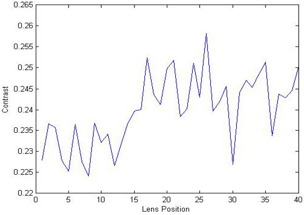
However, under low light conditions, the higher frequency content in a focused image is just a little more than that in the corresponding defocused or blurred image. A focused image obtained from low light conditions possesses a small contrast value and it may be easily influenced by noise. Although we formerly used the modified bilateral filter for noise reduction, it is still necessary to cope with the influence of noise. As illustrated in <xref ref-type="fig" rid="f3-sensors-11-08281">Figure 3</xref>, due to the low contrast of image and noise influence, contrast measurement may generate a fluctuant curve with many local false peaks. In this case, it is difficult to distinguish a well-defined peak, and this hinders the following peak search procedure from performing its function in locating the best focused contrast peak.</p>
<p>As we know, the sharper the focus peak is, the easier it is to find the best focused lens position. Thus bringing in the local false peaks can decrease the noise contribution, and help locating the best focused contrast peak. According to [<xref ref-type="bibr" rid="b6-sensors-11-08281">6</xref>], the second-order function gives better results than higher orders, because of the increase in noise effects. And it is better suited than the first-order difference, as the width of the top of the extremum of the focus function is smaller. Thus we wondered whether an order between first and second variance can be effective. In order to cope with noise and low light conditions, we introduce a contrast measure adaptive to noise influence (CMAN). Our contrast measure is defined based on <xref ref-type="disp-formula" rid="FD3">Equation (3)</xref>, which can be described as follows:
<disp-formula id="FD5">
<label>(5)</label>
<mml:math display="block">
<mml:mrow>
<mml:mi>F</mml:mi>
<mml:mrow>
<mml:mo>(</mml:mo>
<mml:mrow>
<mml:mi>x</mml:mi>
<mml:mrow>
<mml:mo>,</mml:mo>
<mml:mo> </mml:mo>
<mml:mi>y</mml:mi></mml:mrow></mml:mrow>
<mml:mo>)</mml:mo></mml:mrow>
<mml:mo>=</mml:mo>
<mml:mfrac>
<mml:mn>1</mml:mn>
<mml:mrow>
<mml:mi>J</mml:mi>
<mml:mo>*</mml:mo>
<mml:mi>K</mml:mi></mml:mrow></mml:mfrac>
<mml:munderover>
<mml:mo>∑</mml:mo>
<mml:mrow>
<mml:mi>x</mml:mi>
<mml:mo>=</mml:mo>
<mml:mn>1</mml:mn></mml:mrow>
<mml:mi>J</mml:mi></mml:munderover>
<mml:mrow>
<mml:munderover>
<mml:mo>∑</mml:mo>
<mml:mrow>
<mml:mi>y</mml:mi>
<mml:mo>=</mml:mo>
<mml:mn>1</mml:mn></mml:mrow>
<mml:mi>K</mml:mi></mml:munderover>
<mml:mrow>
<mml:mi>G</mml:mi>
<mml:mrow>
<mml:mo>(</mml:mo>
<mml:mrow>
<mml:mi>x</mml:mi>
<mml:mo>,</mml:mo>
<mml:mi>y</mml:mi></mml:mrow>
<mml:mo>)</mml:mo></mml:mrow>
<mml:mrow>
<mml:mo>(</mml:mo>
<mml:mrow>
<mml:mroot>
<mml:mrow>
<mml:mi>G</mml:mi>
<mml:mrow>
<mml:mo>(</mml:mo>
<mml:mrow>
<mml:mi>x</mml:mi>
<mml:mo>,</mml:mo>
<mml:mi>y</mml:mi></mml:mrow>
<mml:mo>)</mml:mo></mml:mrow>
<mml:mo>+</mml:mo>
<mml:mn>1</mml:mn></mml:mrow>
<mml:mi>n</mml:mi></mml:mroot>
<mml:mo>−</mml:mo>
<mml:mn>1</mml:mn></mml:mrow>
<mml:mo>)</mml:mo></mml:mrow></mml:mrow></mml:mrow></mml:mrow></mml:math></disp-formula>where n is computed by:
<disp-formula id="FD6">
<label>(6)</label>
<mml:math display="block">
<mml:mrow>
<mml:mi>n</mml:mi>
<mml:mo>=</mml:mo>
<mml:mrow>
<mml:mo>{</mml:mo>
<mml:mrow>
<mml:mtable>
<mml:mtr>
<mml:mtd columnalign="left">
<mml:mn>1</mml:mn></mml:mtd>
<mml:mtd columnalign="right">
<mml:mrow>
<mml:mi>m</mml:mi>
<mml:mo>≤</mml:mo>
<mml:msub>
<mml:mrow>
<mml:mi>T</mml:mi></mml:mrow>
<mml:mn>1</mml:mn></mml:msub></mml:mrow></mml:mtd></mml:mtr>
<mml:mtr>
<mml:mtd columnalign="left">
<mml:mn>2</mml:mn></mml:mtd>
<mml:mtd columnalign="right">
<mml:mrow>
<mml:msub>
<mml:mrow>
<mml:mi>T</mml:mi></mml:mrow>
<mml:mn>1</mml:mn></mml:msub>
<mml:mo>&lt;</mml:mo>
<mml:mi>m</mml:mi>
<mml:mo>&lt;</mml:mo>
<mml:msub>
<mml:mrow>
<mml:mi>T</mml:mi></mml:mrow>
<mml:mn>2</mml:mn></mml:msub></mml:mrow></mml:mtd></mml:mtr>
<mml:mtr>
<mml:mtd columnalign="left">
<mml:mn>3</mml:mn></mml:mtd>
<mml:mtd columnalign="right">
<mml:mrow>
<mml:mi>m</mml:mi>
<mml:mo>≥</mml:mo>
<mml:msub>
<mml:mrow>
<mml:mi>T</mml:mi></mml:mrow>
<mml:mn>2</mml:mn></mml:msub></mml:mrow></mml:mtd></mml:mtr></mml:mtable></mml:mrow></mml:mrow></mml:mrow></mml:math></disp-formula>where the parameter m is the number of local maximums with value bigger than a predefined threshold T. When m is not more than the parameter T<sub>1</sub>, it means that the noise has little influence on image. We can observe a well defined peak standing for the best focused image. CMSL can work well on this image. In this case, the parameter n is equal to 1, and <xref ref-type="disp-formula" rid="FD5">Equation (5)</xref> is equal to <xref ref-type="disp-formula" rid="FD3">Equation (3)</xref>. If m is more than the parameter T<sub>1</sub> and less than the parameter T<sub>2</sub>, the noise adds a little bias to the contrast measure. At this time, the shape of the curve becomes a little fluctuant due to the noise. It becomes difficult to locate the focus peak due to the absence of a well defined peak. Decreasing the order of contrast measures can help alleviating the noise effects, and bring in local false peaks. As the number of local maxima with big values increases to a certain extent T<sub>2</sub>, the shape of the curve becomes more fluctuant, and it becomes more difficult to locate the best focused image. In this case, a further decrease of the order of contrast measures is necessary.</p>
<p>CMAN is theoretically self-consistent. For a continuous function such as <xref ref-type="disp-formula" rid="FD5">Equation (5)</xref>, its left derivative has the same value to its right derivative from the point <italic>G</italic>(<italic>x</italic>, <italic>y</italic>) = 0 to <italic>G</italic>(<italic>x</italic>, <italic>y</italic>) → +∞. And from <xref ref-type="disp-formula" rid="FD4">Equation (4)</xref>, we can confirm that <italic>G</italic>(<italic>x</italic>, <italic>y</italic>) ≥ 0. According to the definition of derivability [<xref ref-type="bibr" rid="b32-sensors-11-08281">32</xref>], it can thus be derived that <xref ref-type="disp-formula" rid="FD5">Equation (5)</xref> has the function derivability on each point, for example the point <italic>x</italic><sub>0</sub>. Then it is also differential on the point <italic>x</italic><sub>0</sub> [<xref ref-type="bibr" rid="b32-sensors-11-08281">32</xref>]. We can then obtain that [<xref ref-type="bibr" rid="b32-sensors-11-08281">32</xref>]:
<disp-formula id="FD7">
<label>(7)</label>
<mml:math display="block">
<mml:mrow>
<mml:mi mathvariant="italic">dy</mml:mi>
<mml:mo>=</mml:mo>
<mml:msup>
<mml:mi>f</mml:mi>
<mml:mo>′</mml:mo></mml:msup>
<mml:mrow>
<mml:mo stretchy="false">(</mml:mo>
<mml:mrow>
<mml:msub>
<mml:mrow>
<mml:mi>x</mml:mi></mml:mrow>
<mml:mn>0</mml:mn></mml:msub></mml:mrow>
<mml:mo stretchy="false">)</mml:mo></mml:mrow>
<mml:mo>⋅</mml:mo>
<mml:mo>Δ</mml:mo>
<mml:mi>x</mml:mi></mml:mrow></mml:math></disp-formula></p>
<p>As stated in [<xref ref-type="bibr" rid="b32-sensors-11-08281">32</xref>], if Δ<italic>x</italic> is quite small, and under the assumption that ƒ'(<italic>x</italic><sub>0</sub>) ≠ 0, it can be derived that:
<disp-formula id="FD8">
<label>(8)</label>
<mml:math display="block">
<mml:mrow>
<mml:mi mathvariant="italic">dy</mml:mi>
<mml:mo>≈</mml:mo>
<mml:mo>Δ</mml:mo>
<mml:mi>y</mml:mi></mml:mrow></mml:math></disp-formula></p>
<p>By using <xref ref-type="disp-formula" rid="FD7">Equation (7)</xref> in <xref ref-type="disp-formula" rid="FD8">Equation (8)</xref>, it can be derived:
<disp-formula id="FD9">
<label>(9)</label>
<mml:math display="block">
<mml:mrow>
<mml:msup>
<mml:mi>f</mml:mi>
<mml:mo>′</mml:mo></mml:msup>
<mml:mrow>
<mml:mo stretchy="false">(</mml:mo>
<mml:mrow>
<mml:msub>
<mml:mrow>
<mml:mi>x</mml:mi></mml:mrow>
<mml:mn>0</mml:mn></mml:msub></mml:mrow>
<mml:mo stretchy="false">)</mml:mo></mml:mrow>
<mml:mo>⋅</mml:mo>
<mml:mo>Δ</mml:mo>
<mml:mi>x</mml:mi>
<mml:mo>≈</mml:mo>
<mml:mi>f</mml:mi>
<mml:mrow>
<mml:mo stretchy="false">(</mml:mo>
<mml:mrow>
<mml:mi>x</mml:mi>
<mml:mo>+</mml:mo>
<mml:msub>
<mml:mrow>
<mml:mi>x</mml:mi></mml:mrow>
<mml:mn>0</mml:mn></mml:msub></mml:mrow>
<mml:mo stretchy="false">)</mml:mo></mml:mrow>
<mml:mo>−</mml:mo>
<mml:mi>f</mml:mi>
<mml:mrow>
<mml:mo stretchy="false">(</mml:mo>
<mml:mrow>
<mml:msub>
<mml:mrow>
<mml:mi>x</mml:mi></mml:mrow>
<mml:mn>0</mml:mn></mml:msub></mml:mrow>
<mml:mo stretchy="false">)</mml:mo></mml:mrow></mml:mrow></mml:math></disp-formula>and it can be also described as:
<disp-formula id="FD10">
<label>(10)</label>
<mml:math display="block">
<mml:mrow>
<mml:mi>f</mml:mi>
<mml:mrow>
<mml:mo stretchy="false">(</mml:mo>
<mml:mrow>
<mml:mi>x</mml:mi>
<mml:mo>+</mml:mo>
<mml:msub>
<mml:mrow>
<mml:mi>x</mml:mi></mml:mrow>
<mml:mn>0</mml:mn></mml:msub></mml:mrow>
<mml:mo stretchy="false">)</mml:mo></mml:mrow>
<mml:mo>≈</mml:mo>
<mml:mi>f</mml:mi>
<mml:mrow>
<mml:mo stretchy="false">(</mml:mo>
<mml:mrow>
<mml:msub>
<mml:mrow>
<mml:mi>x</mml:mi></mml:mrow>
<mml:mn>0</mml:mn></mml:msub></mml:mrow>
<mml:mo stretchy="false">)</mml:mo></mml:mrow>
<mml:mo>+</mml:mo>
<mml:msup>
<mml:mi>f</mml:mi>
<mml:mo>′</mml:mo></mml:msup>
<mml:mrow>
<mml:mo stretchy="false">(</mml:mo>
<mml:mrow>
<mml:msub>
<mml:mrow>
<mml:mi>x</mml:mi></mml:mrow>
<mml:mn>0</mml:mn></mml:msub></mml:mrow>
<mml:mo stretchy="false">)</mml:mo></mml:mrow>
<mml:mo>⋅</mml:mo>
<mml:mrow>
<mml:mo stretchy="false">(</mml:mo>
<mml:mrow>
<mml:mi>x</mml:mi>
<mml:mo>−</mml:mo>
<mml:msub>
<mml:mrow>
<mml:mi>x</mml:mi></mml:mrow>
<mml:mn>0</mml:mn></mml:msub></mml:mrow>
<mml:mo stretchy="false">)</mml:mo></mml:mrow></mml:mrow></mml:math></disp-formula></p>
<p>If a pixel <italic>x</italic> in an image is from the same homogenous region with its adjacent pixels <italic>y<sub>n</sub></italic> (n = 1, 2, …, 8), then we have <italic>I</italic>(<italic>x</italic>) = <italic>I</italic>(<italic>y<sub>n</sub></italic>). From <xref ref-type="disp-formula" rid="FD4">Equation (4)</xref>, it can be derived that <italic>G</italic>(<italic>x</italic>, <italic>y</italic>) = 0. Thus we set <italic>x</italic><sub>0</sub> = 0 in <xref ref-type="disp-formula" rid="FD10">Equation (10)</xref>, and it can be derived that:
<disp-formula id="FD11">
<label>(11)</label>
<mml:math display="block">
<mml:mrow>
<mml:mi>f</mml:mi>
<mml:mrow>
<mml:mo stretchy="false">(</mml:mo>
<mml:mi>x</mml:mi>
<mml:mo stretchy="false">)</mml:mo></mml:mrow>
<mml:mo>≈</mml:mo>
<mml:mi>f</mml:mi>
<mml:mrow>
<mml:mo stretchy="false">(</mml:mo>
<mml:mn>0</mml:mn>
<mml:mo stretchy="false">)</mml:mo></mml:mrow>
<mml:mo>+</mml:mo>
<mml:msup>
<mml:mi>f</mml:mi>
<mml:mo>′</mml:mo></mml:msup>
<mml:mrow>
<mml:mo stretchy="false">(</mml:mo>
<mml:mn>0</mml:mn>
<mml:mo stretchy="false">)</mml:mo></mml:mrow>
<mml:mo>⋅</mml:mo>
<mml:mi>x</mml:mi></mml:mrow></mml:math></disp-formula></p>
<p>By using <xref ref-type="disp-formula" rid="FD11">Equation (11)</xref> in our proposed contrast measure <xref ref-type="disp-formula" rid="FD5">Equation (5)</xref>, it can be derived that:
<disp-formula id="FD12">
<label>(12)</label>
<mml:math display="block">
<mml:mtable columnalign="left">
<mml:mtr>
<mml:mtd>
<mml:mi>F</mml:mi>
<mml:mrow>
<mml:mo stretchy="false">(</mml:mo>
<mml:mrow>
<mml:mi>x</mml:mi>
<mml:mo>,</mml:mo>
<mml:mi>y</mml:mi></mml:mrow>
<mml:mo stretchy="false">)</mml:mo></mml:mrow></mml:mtd>
<mml:mtd>
<mml:mo>=</mml:mo>
<mml:mfrac>
<mml:mn>1</mml:mn>
<mml:mrow>
<mml:mi>J</mml:mi>
<mml:mo>*</mml:mo>
<mml:mi>K</mml:mi></mml:mrow></mml:mfrac>
<mml:munderover>
<mml:mo>∑</mml:mo>
<mml:mrow>
<mml:mi>x</mml:mi>
<mml:mo>=</mml:mo>
<mml:mn>1</mml:mn></mml:mrow>
<mml:mi>J</mml:mi></mml:munderover>
<mml:mrow>
<mml:munderover>
<mml:mo>∑</mml:mo>
<mml:mrow>
<mml:mi>y</mml:mi>
<mml:mo>=</mml:mo>
<mml:mn>1</mml:mn></mml:mrow>
<mml:mi>K</mml:mi></mml:munderover>
<mml:mi>G</mml:mi>
<mml:mrow>
<mml:mo stretchy="false">(</mml:mo>
<mml:mrow>
<mml:mi>x</mml:mi>
<mml:mo>,</mml:mo>
<mml:mi>y</mml:mi></mml:mrow>
<mml:mo stretchy="false">)</mml:mo></mml:mrow>
<mml:mrow>
<mml:mo>(</mml:mo>
<mml:mrow>
<mml:mroot>
<mml:mrow>
<mml:mi>G</mml:mi>
<mml:mrow>
<mml:mo stretchy="false">(</mml:mo>
<mml:mrow>
<mml:mi>x</mml:mi>
<mml:mo>,</mml:mo>
<mml:mi>y</mml:mi></mml:mrow>
<mml:mo stretchy="false">)</mml:mo></mml:mrow>
<mml:mo>+</mml:mo>
<mml:mn>1</mml:mn></mml:mrow>
<mml:mi>n</mml:mi></mml:mroot>
<mml:mo>−</mml:mo>
<mml:mn>1</mml:mn></mml:mrow>
<mml:mo>)</mml:mo></mml:mrow></mml:mrow></mml:mtd></mml:mtr>
<mml:mtr>
<mml:mtd>
<mml:mrow/></mml:mtd>
<mml:mtd>
<mml:mo>≈</mml:mo>
<mml:mfrac>
<mml:mn>1</mml:mn>
<mml:mrow>
<mml:mi>J</mml:mi>
<mml:mo>*</mml:mo>
<mml:mi>K</mml:mi></mml:mrow></mml:mfrac>
<mml:munderover>
<mml:mo>∑</mml:mo>
<mml:mrow>
<mml:mi>x</mml:mi>
<mml:mo>=</mml:mo>
<mml:mn>1</mml:mn></mml:mrow>
<mml:mi>J</mml:mi></mml:munderover>
<mml:mrow>
<mml:munderover>
<mml:mo>∑</mml:mo>
<mml:mrow>
<mml:mi>y</mml:mi>
<mml:mo>=</mml:mo>
<mml:mn>1</mml:mn></mml:mrow>
<mml:mi>K</mml:mi></mml:munderover>
<mml:mi>G</mml:mi>
<mml:mrow>
<mml:mo stretchy="false">(</mml:mo>
<mml:mrow>
<mml:mi>x</mml:mi>
<mml:mo>,</mml:mo>
<mml:mi>y</mml:mi></mml:mrow>
<mml:mo stretchy="false">)</mml:mo></mml:mrow>
<mml:mo>*</mml:mo>
<mml:mrow>
<mml:mo>(</mml:mo>
<mml:mrow>
<mml:mrow>
<mml:mo>(</mml:mo>
<mml:mrow>
<mml:mroot>
<mml:mrow>
<mml:mn>0</mml:mn>
<mml:mo>+</mml:mo>
<mml:mn>1</mml:mn></mml:mrow>
<mml:mi>n</mml:mi></mml:mroot>
<mml:mo>−</mml:mo>
<mml:mn>1</mml:mn></mml:mrow>
<mml:mo>)</mml:mo></mml:mrow>
<mml:mo>+</mml:mo>
<mml:mrow>
<mml:mo>(</mml:mo>
<mml:mrow>
<mml:mfrac>
<mml:mn>1</mml:mn>
<mml:mi>n</mml:mi></mml:mfrac>
<mml:msup>
<mml:mrow>
<mml:mrow>
<mml:mrow>
<mml:mo stretchy="false">(</mml:mo>
<mml:mrow>
<mml:mn>0</mml:mn>
<mml:mo>+</mml:mo>
<mml:mn>1</mml:mn></mml:mrow>
<mml:mo stretchy="false">)</mml:mo></mml:mrow></mml:mrow></mml:mrow>
<mml:mrow>
<mml:mfrac>
<mml:mn>1</mml:mn>
<mml:mi>n</mml:mi></mml:mfrac>
<mml:mo>−</mml:mo>
<mml:mn>1</mml:mn></mml:mrow></mml:msup></mml:mrow>
<mml:mo>)</mml:mo></mml:mrow>
<mml:mi>G</mml:mi>
<mml:mrow>
<mml:mo stretchy="false">(</mml:mo>
<mml:mrow>
<mml:mi>x</mml:mi>
<mml:mo>,</mml:mo>
<mml:mi>y</mml:mi></mml:mrow>
<mml:mo stretchy="false">)</mml:mo></mml:mrow></mml:mrow>
<mml:mo>)</mml:mo></mml:mrow></mml:mrow></mml:mtd></mml:mtr>
<mml:mtr>
<mml:mtd>
<mml:mrow/></mml:mtd>
<mml:mtd>
<mml:mo>=</mml:mo>
<mml:mfrac>
<mml:mn>1</mml:mn>
<mml:mrow>
<mml:mi>J</mml:mi>
<mml:mo>*</mml:mo>
<mml:mi>K</mml:mi>
<mml:mo>*</mml:mo>
<mml:mi>n</mml:mi></mml:mrow></mml:mfrac>
<mml:munderover>
<mml:mo>∑</mml:mo>
<mml:mrow>
<mml:mi>x</mml:mi>
<mml:mo>=</mml:mo>
<mml:mn>1</mml:mn></mml:mrow>
<mml:mi>J</mml:mi></mml:munderover>
<mml:mrow>
<mml:munderover>
<mml:mo>∑</mml:mo>
<mml:mrow>
<mml:mi>y</mml:mi>
<mml:mo>=</mml:mo>
<mml:mn>1</mml:mn></mml:mrow>
<mml:mi>K</mml:mi></mml:munderover>
<mml:mi>G</mml:mi>
<mml:msup>
<mml:mrow>
<mml:mrow>
<mml:mrow>
<mml:mo stretchy="false">(</mml:mo>
<mml:mrow>
<mml:mi>x</mml:mi>
<mml:mo>,</mml:mo>
<mml:mi>y</mml:mi></mml:mrow>
<mml:mo stretchy="false">)</mml:mo></mml:mrow></mml:mrow></mml:mrow>
<mml:mn>2</mml:mn></mml:msup>
<mml:mo>=</mml:mo>
<mml:mfrac>
<mml:mn>1</mml:mn>
<mml:mi>n</mml:mi></mml:mfrac>
<mml:mi>L</mml:mi>
<mml:mrow>
<mml:mo stretchy="false">(</mml:mo>
<mml:mrow>
<mml:mi>x</mml:mi>
<mml:mo>,</mml:mo>
<mml:mi>y</mml:mi></mml:mrow>
<mml:mo stretchy="false">)</mml:mo></mml:mrow></mml:mrow></mml:mtd></mml:mtr></mml:mtable></mml:math></disp-formula></p>
<p>By using <xref ref-type="disp-formula" rid="FD6">Equation (6)</xref> in <xref ref-type="disp-formula" rid="FD12">Equation (12)</xref>, and under the assumption that pixels in image are from the same homogenous region with its adjacent pixels, it can be derived that:
<disp-formula id="FD13">
<label>(13)</label>
<mml:math display="block">
<mml:mrow>
<mml:mi>F</mml:mi>
<mml:mrow>
<mml:mo stretchy="false">(</mml:mo>
<mml:mrow>
<mml:mi>x</mml:mi>
<mml:mo>,</mml:mo>
<mml:mi>y</mml:mi></mml:mrow>
<mml:mo stretchy="false">)</mml:mo></mml:mrow>
<mml:mo>≈</mml:mo>
<mml:mrow>
<mml:mo>{</mml:mo>
<mml:mrow>
<mml:mtable>
<mml:mtr>
<mml:mtd columnalign="left">
<mml:mrow>
<mml:mi>L</mml:mi>
<mml:mrow>
<mml:mo stretchy="false">(</mml:mo>
<mml:mrow>
<mml:mi>x</mml:mi>
<mml:mo>,</mml:mo>
<mml:mi>y</mml:mi></mml:mrow>
<mml:mo stretchy="false">)</mml:mo></mml:mrow></mml:mrow></mml:mtd>
<mml:mtd columnalign="right">
<mml:mrow>
<mml:mi>m</mml:mi>
<mml:mo>≤</mml:mo>
<mml:msub>
<mml:mrow>
<mml:mi>T</mml:mi></mml:mrow>
<mml:mn>1</mml:mn></mml:msub></mml:mrow></mml:mtd></mml:mtr>
<mml:mtr columnalign="left">
<mml:mtd columnalign="right">
<mml:mrow>
<mml:mfrac>
<mml:mn>1</mml:mn>
<mml:mn>2</mml:mn></mml:mfrac>
<mml:mi>L</mml:mi>
<mml:mrow>
<mml:mo stretchy="false">(</mml:mo>
<mml:mrow>
<mml:mi>x</mml:mi>
<mml:mo>,</mml:mo>
<mml:mi>y</mml:mi></mml:mrow>
<mml:mo stretchy="false">)</mml:mo></mml:mrow></mml:mrow></mml:mtd>
<mml:mtd columnalign="right">
<mml:mrow>
<mml:msub>
<mml:mrow>
<mml:mi>T</mml:mi></mml:mrow>
<mml:mn>1</mml:mn></mml:msub>
<mml:mo>&lt;</mml:mo>
<mml:mi>m</mml:mi>
<mml:mo>&lt;</mml:mo>
<mml:msub>
<mml:mrow>
<mml:mi>T</mml:mi></mml:mrow>
<mml:mn>2</mml:mn></mml:msub></mml:mrow></mml:mtd></mml:mtr>
<mml:mtr>
<mml:mtd columnalign="left">
<mml:mrow>
<mml:mfrac>
<mml:mn>1</mml:mn>
<mml:mn>3</mml:mn></mml:mfrac>
<mml:mi>L</mml:mi>
<mml:mrow>
<mml:mo stretchy="false">(</mml:mo>
<mml:mrow>
<mml:mi>x</mml:mi>
<mml:mo>,</mml:mo>
<mml:mi>y</mml:mi></mml:mrow>
<mml:mo stretchy="false">)</mml:mo></mml:mrow></mml:mrow></mml:mtd>
<mml:mtd columnalign="right">
<mml:mrow>
<mml:mi>m</mml:mi>
<mml:mo>≥</mml:mo>
<mml:msub>
<mml:mrow>
<mml:mi>T</mml:mi></mml:mrow>
<mml:mn>2</mml:mn></mml:msub></mml:mrow></mml:mtd></mml:mtr></mml:mtable></mml:mrow></mml:mrow></mml:mrow></mml:math></disp-formula></p>
<p><xref ref-type="disp-formula" rid="FD13">Equation (13)</xref> means that the value of CMAN decreases when the noise contributions increase. When an image is little influenced by noise, CMAN has almost the same value as CMSL. As stated previously, when noise adds a little bias to the image, the shape of the curve becomes a little fluctuant. In this case, the value of CMAN decreases to almost half the value of CMSL. This means a decrease of the value of local false peaks, and therefore the curve shape becomes flat in the homogenous region. When noise adds more bias to the image, CMAN has even less value than CMSL. As a result, CMAN brings in the peak of local maximum caused by the noise influence and a well-defined focus peak can thus be produced.</p></sec>
<sec>
<label>3.3.</label>
<title>Peak Search</title>
<p>While the focusing accuracy is dependent on the contrast measure used, the reliability and speed of an AF algorithm depend on the peak search algorithm. Various peak search algorithms were presented in the past, such as global search, Fibonacci search [<xref ref-type="bibr" rid="b11-sensors-11-08281">11</xref>], coarse-to-fine search [<xref ref-type="bibr" rid="b33-sensors-11-08281">33</xref>], and rule-based search [<xref ref-type="bibr" rid="b5-sensors-11-08281">5</xref>]. For a low contrast image, the contrast difference of the images obtained in different lens positions is quite small. It is difficult to decide when it is suitable to search the focus range using a big step size, thus coarse-to-fine search and rule-based search cannot work well in low light conditions. Global search scans the entire focus range with the smallest motor step in a forward manner. The main advantage of this algorithm is that there is no possibility of falsely obtaining a local peak since all focus positions are examined. However, each evaluation of the criterion function is a relatively expensive operation; it needs to minimize the number of evaluations required. For this reason, global search is not a feasible strategy. Fibonacci search uses the Fibonacci numbers to scan lens positions, and can achieve good convergence speed. However, it reverses the search direction too many times and thus possesses high power consumption [<xref ref-type="bibr" rid="b5-sensors-11-08281">5</xref>].</p>
<p>In order to make the peak search robust to low light conditions, tradeoffs in terms of focusing reliability, convergence speed, and power consumption should be made. We adopt the AF peak search algorithm proposed by Li in [<xref ref-type="bibr" rid="b1-sensors-11-08281">1</xref>], which takes account of the limited resolution of human visual systems. As stated in [<xref ref-type="bibr" rid="b1-sensors-11-08281">1</xref>], the focus is acceptable when it is 12 μm (corresponding to four times the smallest moving step) off the peak. Thus we scan the entire focus range in a forward direction using four motor steps at each movement. Departing from Li who used stop criteria to expedite the convergence speed, the peak search procedure will not terminate until the last lens position to ensure the focusing reliability under low light conditions. This peak search has enough convergence speed because it is not an exhaustive search. In addition, because the search does not always start from the home position; therefore it could avoid blur experience and saves energy [<xref ref-type="bibr" rid="b1-sensors-11-08281">1</xref>].</p></sec>
<sec>
<label>3.4.</label>
<title>Procedure of the Proposed AF Algorithm</title>
<p>As illustrated in <xref ref-type="fig" rid="f4-sensors-11-08281">Figure 4</xref>, after the noise reduction preprocessing, contrasts of image sequence are computed using CMSL. We can then calculate the number of local maxima with big contrast values. As a result, the parameter m can be obtained. If m is less than the parameter T<sub>1</sub>, it can observe a well defined peak with a maximum contrast value standing for the best focused image. Otherwise, we compare m to the parameter T<sub>2</sub> to obtain the value of n, and calculate the image contrast using CMAN according to the parameter n. After that, a peak search procedure is performed to locating the best focused image. In this case, CMAN can alleviate the noise influence, and at the same time produce a well-defined focus peak. Although the contrast computation is a little more complex than CMSL, the computation time is acceptable and will not cause any lag in our passive AF system. In addition, the dedicated hardware architecture for real-time auto-focusing, such as field programmable gate array (FPGA)-based AF system [<xref ref-type="bibr" rid="b34-sensors-11-08281">34</xref>], can be used to shorten the computation time, which processes the incoming pixels simultaneously with their neighboring pixels based on its parallelized window processing architecture. The extra computation in CMAN aims to distinguish the best focused peak from noise influence which is critical to ensure the focusing accuracy and reliability. Thus it is a suitable measurement for gauge the effectiveness of our passive AF algorithm in improving the performance under low light conditions.</p></sec></sec>
<sec sec-type="results">
<label>4.</label>
<title>Experiments and Results</title>
<p>
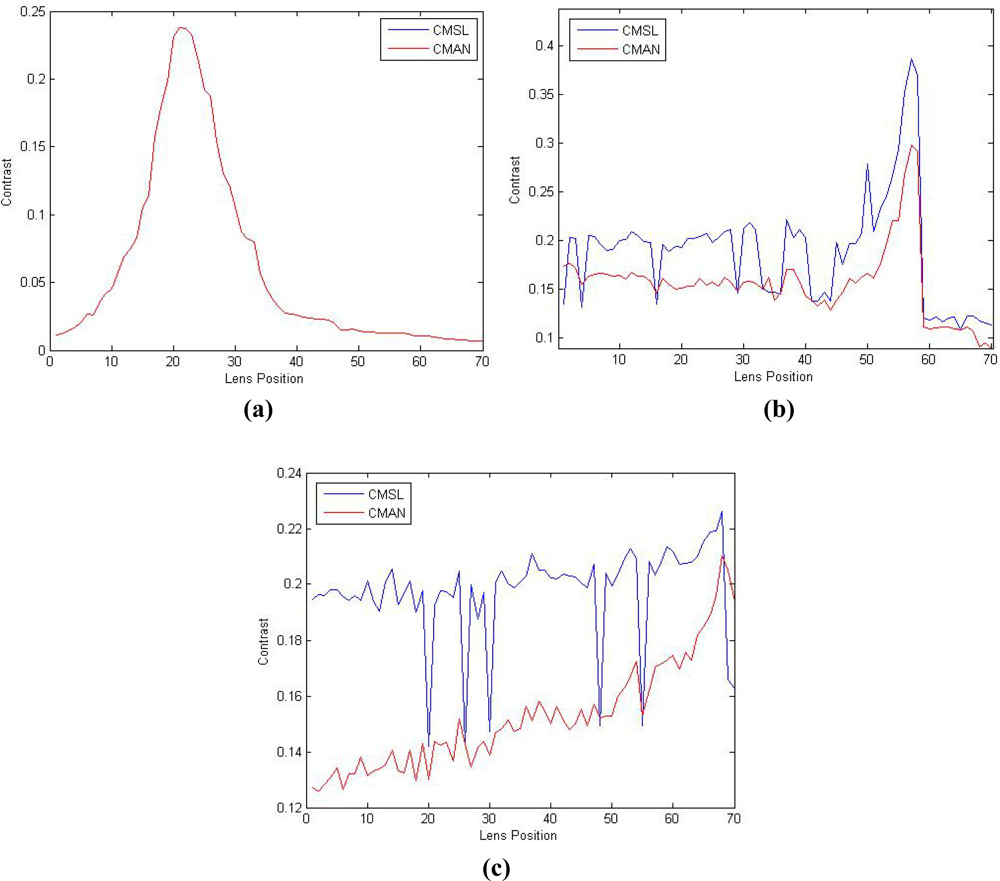
In the experiments, the objects A, B, and C (<xref ref-type="fig" rid="f5-sensors-11-08281">Figure 5</xref>) were autofocused in different lens positions using our proposed passive AF algorithm, from defocusing to focusing and from focusing to defocusing. Three different image sequences can be obtained, which were used to investigate the performance of CMAN. The three image sequences are representative for a certain class of image types, including low contrast image with little noise influence (object A), low contrast image with adequate noise (object B) and low contrast image corrupted by much noise (object C). The noise can be either additive noise or multiplicative noise. CMAN and CMSL were tested in the experiments, where T is set to be half value of the focused peak in CMSL, T<sub>1</sub> is set to be 1 indicating just one well defined peak, and T<sub>2</sub> is set to be 9 standing for the presence of adequate noise. In order to evaluate the performance of CMAN and CMSL, noise reduction preprocessing and peak search procedure were implemented in all of the tests. From the previous discussion, it can be expected that CMAN and CMSL would response differently towards these image sequences.</p>
<p>In the first experiment, the resulting contrast value is plotted against 70 different lens positions in a consumer level digital camera, from near to far. As illustrated in <xref ref-type="fig" rid="f6-sensors-11-08281">Figure 6(a)</xref>, CMSL and CMAN have the same contrast value in all the 70 lens positions when the image is little influenced by noise. And it can witness a well defined focus peak in the 21st lens position.</p>
<p>In the second experiment, the low contrast image with adequate noise influence acquired at 70 different lens positions from near to far is used for this experiment. The results are shown in <xref ref-type="fig" rid="f6-sensors-11-08281">Figure 6(b)</xref>, where the 57th lens position is the one with the best contrast. As we can see, when noise has a little influence on the image, the curve generated by CMSL is more fluctuant than CMAN and we can observe a local false peak with a big value in the 50th lens position of the curve produced by CMSL. In this case, it is difficult to distinguish the focus peak from this local false peak. Differently, CMAN can decrease the value of local false peak and works well in this image. As illustrated in <xref ref-type="fig" rid="f6-sensors-11-08281">Figure 6(b)</xref>, although there are still a number of local false peaks, their value is relatively small and they can be distinguished from the focused peak. In other words, CMAN brings in the peak of local maximum caused by the noise influence, and produces a well-defined focus peak.</p>
<p>In the last experiment, the low contrast image is corrupted by much noise. We also capture the image sequence at 70 different lens positions from near to far. The 68th lens position is the one with the best contrast. The results shown in <xref ref-type="fig" rid="f6-sensors-11-08281">Figure 6(c)</xref> clearly indicate that CMAN has more robust performance than CMSL. While CMSL fails, CMAN is still able to determine correctly the focus position.</p></sec>
<sec sec-type="conclusions">
<label>5.</label>
<title>Conclusions</title>
<p>This paper has described a robust passive AF algorithm using a new contrast measurement. The proposed algorithm is robust to both additive noise and multiplicative noise, and can provide a noticeable improvement in discrimination performance under low light conditions. The experimental results from an actual digital camera deployment validate the theory developed to distinguish the focus peak from local false peaks.</p></sec></body>
<back>
<ack>
<p>This work was supported in part by the Program of Wuhan Subject Chief Scientist (201150530152), the Open Foundation (2010D11) of State Key Laboratory of Bioelectronics, the Educational Commission of Hubei Province (Q20101101, Q20101110), the National High-tech Research and Development Project of China (863) under the grant 2009AA04Z106, the Educational Commission of Hubei Province (D20091102), the projects (2009CDA034, 2009CDA136, 2008CDB345) from the Natural Science Foundation of Hubei Provincial of China, the Natural Science Foundation of China (60803160, 60773088, 60975031), and the Project (2008TD04) from Science Foundation of Wuhan University of Science and Technology.</p></ack>
<ref-list>
<title>References</title>
<ref id="b1-sensors-11-08281"><label>1.</label><citation citation-type="journal"><person-group person-group-type="author"><name><surname>Li</surname><given-names>J</given-names></name></person-group><article-title>Autofocus searching algorithm considering human visual system limitations</article-title><source>Opt. Eng</source><year>2005</year><volume>44</volume><fpage>113201</fpage><pub-id pub-id-type="doi">10.1117/1.2130725</pub-id></citation></ref>
<ref id="b2-sensors-11-08281"><label>2.</label><citation citation-type="journal"><person-group person-group-type="author"><name><surname>Ni</surname><given-names>J</given-names></name><name><surname>Wei</surname><given-names>M</given-names></name><name><surname>Yuan</surname><given-names>J</given-names></name><name><surname>Wu</surname><given-names>Q</given-names></name></person-group><article-title>Efficient auto-focus algorithm for optical measurement system</article-title><source>Proc. SPIE</source><year>2009</year><volume>7283</volume><fpage>728344</fpage></citation></ref>
<ref id="b3-sensors-11-08281"><label>3.</label><citation citation-type="journal"><person-group person-group-type="author"><name><surname>Gamadia</surname><given-names>M</given-names></name><name><surname>Kehtarnavaz</surname><given-names>N</given-names></name><name><surname>Roberts-Hoffman</surname><given-names>K</given-names></name></person-group><article-title>Low-light auto-focus enhancement for digital and cell-phone camera image pipelines</article-title><source>IEEE Trans. Consum. Electron</source><year>2007</year><volume>53</volume><fpage>249</fpage><lpage>257</lpage><pub-id pub-id-type="doi">10.1109/TCE.2007.381682</pub-id></citation></ref>
<ref id="b4-sensors-11-08281"><label>4.</label><citation citation-type="journal"><person-group person-group-type="author"><name><surname>Shih</surname><given-names>L</given-names></name></person-group><article-title>Autofocus survey: A comparison of algorithms</article-title><source>Proc. SPIE</source><year>2007</year><volume>6502</volume><fpage>65020B</fpage></citation></ref>
<ref id="b5-sensors-11-08281"><label>5.</label><citation citation-type="journal"><person-group person-group-type="author"><name><surname>Kehtarnavaz</surname><given-names>N</given-names></name><name><surname>Oh</surname><given-names>HJ</given-names></name></person-group><article-title>Development and real-time implementation of a rule-based auto-focus algorithm</article-title><source>Real Time Imag</source><year>2003</year><volume>9</volume><fpage>197</fpage><lpage>203</lpage><pub-id pub-id-type="doi">10.1016/S1077-2014(03)00037-8</pub-id></citation></ref>
<ref id="b6-sensors-11-08281"><label>6.</label><citation citation-type="journal"><person-group person-group-type="author"><name><surname>Groen</surname><given-names>FCA</given-names></name><name><surname>Young</surname><given-names>IT</given-names></name><name><surname>Ligthart</surname><given-names>G</given-names></name></person-group><article-title>A comparison of different autofocus algorithms</article-title><source>Cytometry</source><year>1985</year><volume>6</volume><fpage>81</fpage><lpage>91</lpage><pub-id pub-id-type="doi">10.1002/cyto.990060202</pub-id><pub-id pub-id-type="pmid">3979220</pub-id></citation></ref>
<ref id="b7-sensors-11-08281"><label>7.</label><citation citation-type="journal"><person-group person-group-type="author"><name><surname>Peddigari</surname><given-names>V</given-names></name><name><surname>Gamadia</surname><given-names>M</given-names></name><name><surname>Kehtarnavaz</surname><given-names>N</given-names></name></person-group><article-title>Real-time implementation issues in passive automatic focusing for digital still cameras</article-title><source>J. Imag. Sci. Technol</source><year>2005</year><volume>49</volume><fpage>114</fpage><lpage>123</lpage></citation></ref>
<ref id="b8-sensors-11-08281"><label>8.</label><citation citation-type="confproc"><person-group person-group-type="author"><name><surname>Chern</surname><given-names>NK</given-names></name><name><surname>Neow</surname><given-names>PA</given-names></name><name><surname>Ang</surname><given-names>MH</given-names><suffix>Jr</suffix></name></person-group><article-title>Practical Issues in Pixel-Based Autofocusing for Machine Vision</article-title><conf-name>Proceedings of IEEE International Conference on Robotics and Automation</conf-name><conf-loc>Seoul, Korea</conf-loc><conf-date>21–26 May 2001</conf-date><fpage>2791</fpage><lpage>2796</lpage></citation></ref>
<ref id="b9-sensors-11-08281"><label>9.</label><citation citation-type="other"><person-group person-group-type="author"><name><surname>Tenenbaum</surname><given-names>JM</given-names></name></person-group><article-title>Accommodation in Computer Vision</article-title><comment>PhD Thesis,</comment><publisher-name>Stanford University</publisher-name><publisher-loc>Stanford, CA, USA</publisher-loc><year>1970</year></citation></ref>
<ref id="b10-sensors-11-08281"><label>10.</label><citation citation-type="book"><person-group person-group-type="author"><name><surname>Schlag</surname><given-names>JF</given-names></name><name><surname>Sanderson</surname><given-names>AC</given-names></name><name><surname>Neumann</surname><given-names>CP</given-names></name><name><surname>Wimberly</surname><given-names>FC</given-names></name></person-group><source>Implementation of Automatic Focusing Algorithms for a Computer Vision System with Camera Control</source><comment>Technical Report CMU-RI-TR-83-14;</comment><publisher-name>Carnegie Mellon University</publisher-name><publisher-loc>Pittsburgh, PA, USA</publisher-loc><year>1983</year></citation></ref>
<ref id="b11-sensors-11-08281"><label>11.</label><citation citation-type="journal"><person-group person-group-type="author"><name><surname>Krotkov</surname><given-names>E</given-names></name></person-group><article-title>Focusing</article-title><source>Int. J. Comput. Vision</source><year>1987</year><volume>1</volume><fpage>223</fpage><lpage>237</lpage></citation></ref>
<ref id="b12-sensors-11-08281"><label>12.</label><citation citation-type="confproc"><person-group person-group-type="author"><name><surname>Baina</surname><given-names>J</given-names></name><name><surname>Dublet</surname><given-names>J</given-names></name></person-group><article-title>Automatic Focus and Iris Control for Cameras</article-title><conf-name>Proceedings of IEEE Fifth International Conference on Image Processing and Its Applications</conf-name><conf-loc>Edinburgh, UK</conf-loc><conf-date>4–6 July 1995</conf-date><fpage>232</fpage><lpage>235</lpage></citation></ref>
<ref id="b13-sensors-11-08281"><label>13.</label><citation citation-type="confproc"><person-group person-group-type="author"><name><surname>Shen</surname><given-names>CH</given-names></name><name><surname>Chen</surname><given-names>HH</given-names></name></person-group><article-title>Robust focus measure for low-contrast images</article-title><conf-name>Proceedings of IEEE International Conference on Consumer Electronics</conf-name><conf-loc>Las Vegas, NV, USA</conf-loc><conf-date>7–11 January 2006</conf-date></citation></ref>
<ref id="b14-sensors-11-08281"><label>14.</label><citation citation-type="confproc"><person-group person-group-type="author"><name><surname>Lee</surname><given-names>ME</given-names></name><name><surname>Chen</surname><given-names>CF</given-names></name><name><surname>Lin</surname><given-names>TN</given-names></name><name><surname>Chen</surname><given-names>CN</given-names></name></person-group><article-title>The application of discrete cosine transform (DCT) combined with the nonlinear regression routine on optical auto-focusing</article-title><conf-name>Proceedings of IEEE International Conference on Consumer Electronics</conf-name><conf-loc>Las Vegas, NV, USA</conf-loc><conf-date>10–14 January 2009</conf-date></citation></ref>
<ref id="b15-sensors-11-08281"><label>15.</label><citation citation-type="journal"><person-group person-group-type="author"><name><surname>Kristan</surname><given-names>M</given-names></name><name><surname>Pers</surname><given-names>J</given-names></name><name><surname>Perse</surname><given-names>M</given-names></name><name><surname>Kovacic</surname><given-names>S</given-names></name></person-group><article-title>A Bayes-spectral-entropy-based measure of camera focus using a discrete cosine transform</article-title><source>Patt. Recogn. Lett</source><year>2006</year><volume>27</volume><fpage>1431</fpage><lpage>1439</lpage><pub-id pub-id-type="doi">10.1016/j.patrec.2006.01.016</pub-id></citation></ref>
<ref id="b16-sensors-11-08281"><label>16.</label><citation citation-type="journal"><person-group person-group-type="author"><name><surname>Lee</surname><given-names>SY</given-names></name><name><surname>Yoo</surname><given-names>JT</given-names></name><name><surname>Kumar</surname><given-names>Y</given-names></name><name><surname>Kim</surname><given-names>SW</given-names></name></person-group><article-title>Reduced energy-ratio measure for robust autofocusing in digital camera</article-title><source>IEEE Sign. Process. Lett</source><year>2009</year><volume>16</volume><fpage>133</fpage><lpage>136</lpage><pub-id pub-id-type="doi">10.1109/LSP.2008.2008938</pub-id></citation></ref>
<ref id="b17-sensors-11-08281"><label>17.</label><citation citation-type="journal"><person-group person-group-type="author"><name><surname>Luo</surname><given-names>Y</given-names></name><name><surname>Ward</surname><given-names>RK</given-names></name></person-group><article-title>Removing the blocking artifacts of block-based DCT compressed images</article-title><source>IEEE Trans. Image Process</source><year>2003</year><volume>12</volume><fpage>838</fpage><lpage>842</lpage><pub-id pub-id-type="doi">10.1109/TIP.2003.814252</pub-id><pub-id pub-id-type="pmid">18237958</pub-id></citation></ref>
<ref id="b18-sensors-11-08281"><label>18.</label><citation citation-type="journal"><person-group person-group-type="author"><name><surname>Lin</surname><given-names>KC</given-names></name></person-group><article-title>Microscopic autofocusing using regional monotonous variations of multiple focal value measures</article-title><source>J. Electron. Imag</source><year>2010</year><volume>19</volume><fpage>023012</fpage><pub-id pub-id-type="doi">10.1117/1.3429726</pub-id></citation></ref>
<ref id="b19-sensors-11-08281"><label>19.</label><citation citation-type="book"><source>Advantages of Power Leds in Cameraphone Applications</source><publisher-name>Philips Lumileds Lighting Company</publisher-name><publisher-loc>San Jose, CA, USA</publisher-loc><year>2006</year></citation></ref>
<ref id="b20-sensors-11-08281"><label>20.</label><citation citation-type="other"><person-group person-group-type="author"><name><surname>Gotanda</surname><given-names>Y</given-names></name></person-group><article-title>Image Capturing Apparatus and Method for Setting Exposure for AF Control Executed by Image Capturing Apparatus</article-title><comment>US Patent 7321395,</comment><day>22</day><month>January</month><year>2008</year></citation></ref>
<ref id="b21-sensors-11-08281"><label>21.</label><citation citation-type="journal"><person-group person-group-type="author"><name><surname>Lim</surname><given-names>SK</given-names></name></person-group><article-title>Characterization of noise in digital photographs for image processing</article-title><source>Proc. SPIE</source><year>2006</year><volume>6069</volume><fpage>219</fpage><lpage>228</lpage></citation></ref>
<ref id="b22-sensors-11-08281"><label>22.</label><citation citation-type="journal"><person-group person-group-type="author"><name><surname>Tang</surname><given-names>J</given-names></name><name><surname>Xu</surname><given-names>X</given-names></name></person-group><article-title>An automatic focus algorithm for still and video camera applications using a new contrast measure</article-title><source>Proc. SPIE</source><year>2009</year><volume>7498</volume><fpage>74984X</fpage></citation></ref>
<ref id="b23-sensors-11-08281"><label>23.</label><citation citation-type="book"><person-group person-group-type="author"><name><surname>Gonzales</surname><given-names>R</given-names></name><name><surname>Woods</surname><given-names>R</given-names></name></person-group><source>Digital Image Processing</source><publisher-name>Prentice-Hall</publisher-name><publisher-loc>Saddle River, NJ, USA</publisher-loc><year>2002</year></citation></ref>
<ref id="b24-sensors-11-08281"><label>24.</label><citation citation-type="book"><person-group person-group-type="author"><name><surname>Bose</surname><given-names>T</given-names></name></person-group><source>Digital Signal and Image Processing</source><publisher-name>John Wiley &amp; Sons</publisher-name><publisher-loc>Hoboken, NJ, USA</publisher-loc><year>2004</year></citation></ref>
<ref id="b25-sensors-11-08281"><label>25.</label><citation citation-type="confproc"><person-group person-group-type="author"><name><surname>Phelippeau</surname><given-names>H</given-names></name><name><surname>Talbot</surname><given-names>H</given-names></name><name><surname>Akil</surname><given-names>M</given-names></name><name><surname>Bara</surname><given-names>S</given-names></name></person-group><article-title>Shot Noise Adaptive Bilateral Filter</article-title><conf-name>Proceedings of the 9th International Conference on Signal Processing</conf-name><conf-loc>Beijing, China</conf-loc><conf-date>26–29 October 2008</conf-date><fpage>864</fpage><lpage>867</lpage></citation></ref>
<ref id="b26-sensors-11-08281"><label>26.</label><citation citation-type="journal"><person-group person-group-type="author"><name><surname>Barash</surname><given-names>D</given-names></name></person-group><article-title>Fundamental relationship between bilateral filtering, adaptive smoothing, and the nonlinear diffusion equation</article-title><source>IEEE Trans. Patt. Anal. Mach. Intell</source><year>2002</year><volume>24</volume><fpage>844</fpage><lpage>847</lpage><pub-id pub-id-type="doi">10.1109/TPAMI.2002.1008390</pub-id></citation></ref>
<ref id="b27-sensors-11-08281"><label>27.</label><citation citation-type="confproc"><person-group person-group-type="author"><name><surname>Tomasi</surname><given-names>C</given-names></name><name><surname>Manduchi</surname><given-names>R</given-names></name></person-group><article-title>Bilateral filtering for gray and color images</article-title><conf-name>Proceedings of International Conference on Computer Vision</conf-name><conf-loc>Bombay, India</conf-loc><conf-date>4–7 January 1998</conf-date><fpage>839</fpage><lpage>846</lpage></citation></ref>
<ref id="b28-sensors-11-08281"><label>28.</label><citation citation-type="journal"><person-group person-group-type="author"><name><surname>Yu</surname><given-names>Y</given-names></name><name><surname>Acton</surname><given-names>ST</given-names></name></person-group><article-title>Speckle reducing anisotropic diffusion</article-title><source>IEEE Trans. Image Process</source><year>2002</year><volume>11</volume><fpage>1260</fpage><lpage>1270</lpage><pub-id pub-id-type="doi">10.1109/TIP.2002.804276</pub-id><pub-id pub-id-type="pmid">18249696</pub-id></citation></ref>
<ref id="b29-sensors-11-08281"><label>29.</label><citation citation-type="journal"><person-group person-group-type="author"><name><surname>Sun</surname><given-names>Q</given-names></name><name><surname>Hossack</surname><given-names>J</given-names></name><name><surname>Tang</surname><given-names>J</given-names></name><name><surname>Acton</surname><given-names>ST</given-names></name></person-group><article-title>Speckle reducing anisotropic diffusion for 3D ultrasound images</article-title><source>Comput. Med. Imag. Graph</source><year>2004</year><volume>28</volume><fpage>461</fpage><lpage>470</lpage></citation></ref>
<ref id="b30-sensors-11-08281"><label>30.</label><citation citation-type="journal"><person-group person-group-type="author"><name><surname>Wachowiak</surname><given-names>S</given-names></name><name><surname>Smolikova</surname><given-names>R</given-names></name><name><surname>Zurada</surname><given-names>J</given-names></name><name><surname>Elmaghraby</surname><given-names>A</given-names></name></person-group><article-title>A neural approach to speckle noise modeling</article-title><source>Intell. Eng. Syst. Artif. Neural Netw</source><year>2000</year><volume>10</volume><fpage>837</fpage><lpage>842</lpage></citation></ref>
<ref id="b31-sensors-11-08281"><label>31.</label><citation citation-type="journal"><person-group person-group-type="author"><name><surname>Tang</surname><given-names>J</given-names></name><name><surname>Guo</surname><given-names>S</given-names></name><name><surname>Sun</surname><given-names>Q</given-names></name><name><surname>Deng</surname><given-names>Y</given-names></name><name><surname>Zhou</surname><given-names>D</given-names></name></person-group><article-title>Speckle reducing bilateral filter for cattle follicle segmentation</article-title><source>BMC Genomics</source><year>2010</year><volume>11</volume><pub-id pub-id-type="doi">10.1186/1471-2164-11-S2-S9</pub-id></citation></ref>
<ref id="b32-sensors-11-08281"><label>32.</label><citation citation-type="book"><person-group person-group-type="author"><name><surname>Apostol</surname><given-names>TM</given-names></name></person-group><source>Mathematical Analysis</source><publisher-name>Addison-Wesley</publisher-name><publisher-loc>Reading, MA, USA</publisher-loc><year>2004</year></citation></ref>
<ref id="b33-sensors-11-08281"><label>33.</label><citation citation-type="journal"><person-group person-group-type="author"><name><surname>He</surname><given-names>J</given-names></name><name><surname>Zhou</surname><given-names>R</given-names></name><name><surname>Hong</surname><given-names>Z</given-names></name></person-group><article-title>Modified fast climbing search auto-focus algorithm with adaptive step size searching technique for digital camera</article-title><source>IEEE Trans. Consum. Electron</source><year>2003</year><volume>49</volume><fpage>257</fpage><lpage>262</lpage><pub-id pub-id-type="doi">10.1109/TCE.2003.1209511</pub-id></citation></ref>
<ref id="b34-sensors-11-08281"><label>34.</label><citation citation-type="journal"><person-group person-group-type="author"><name><surname>Jin</surname><given-names>S</given-names></name><name><surname>Cho</surname><given-names>J</given-names></name><name><surname>Kwon</surname><given-names>KH</given-names></name><name><surname>Jeon</surname><given-names>JW</given-names></name></person-group><article-title>A dedicated hardware architecture for real-time auto-focusing using an FPGA</article-title><source>Mach. Vision Appl</source><year>2010</year><volume>21</volume><fpage>727</fpage><lpage>734</lpage><pub-id pub-id-type="doi">10.1007/s00138-009-0190-2</pub-id></citation></ref></ref-list>
<sec sec-type="display-objects">
<title>Figures</title>
<fig id="f1-sensors-11-08281" position="float">
<label>Figure 1.</label>
<caption>
<p>Traditional passive AF system.</p></caption>
<graphic xlink:href="sensors-11-08281f1.gif"/></fig>
<fig id="f2-sensors-11-08281" position="float">
<label>Figure 2.</label>
<caption>
<p>Image contrasts at different lens position.</p></caption>
<graphic xlink:href="sensors-11-08281f2.gif"/></fig>
<fig id="f3-sensors-11-08281" position="float">
<label>Figure 3.</label>
<caption>
<p>Influence of noise on the shape of a low contrast image.</p></caption>
<graphic xlink:href="sensors-11-08281f3.gif"/></fig>
<fig id="f4-sensors-11-08281" position="float">
<label>Figure 4.</label>
<caption>
<p>Proposed passive AF algorithm using CMAN.</p></caption>
<graphic xlink:href="sensors-11-08281f4.gif"/></fig>
<fig id="f5-sensors-11-08281" position="float">
<label>Figure 5.</label>
<caption>
<p>Image used in the experiments <bold>(a)</bold> Object A. <bold>(b)</bold> Object B. <bold>(c)</bold> Object C.</p></caption>
<graphic xlink:href="sensors-11-08281f5.gif"/></fig>
<fig id="f6-sensors-11-08281" position="float">
<label>Figure 6.</label>
<caption>
<p>The shape of a low contrast image obtained by CMSL and CMAN <bold>(a)</bold> under little noise conditions; <bold>(b)</bold> under adequate noise conditions; <bold>(c)</bold> under much noise conditions.</p></caption>
<graphic xlink:href="sensors-11-08281f6.gif"/></fig></sec></back></article>
