Optimal Rate Allocation in Cluster-Tree WSNs

 ,
, 
 ,
,
Abstract
: In this paper, we propose a solution to the problem of guaranteed time slot allocation in cluster-tree WSNs. Our design uses the so-called Network Utility Maximization (NUM) approach as far as we aim to provide a fair distribution of the available resources. From the point of view of implementation, we extend here the authors’ proposed Coupled-Decompositions Method (CDM) in order to compute the NUM problem inside the cluster tree topology and we prove the optimality of this new extended version of the method. As a result, we obtain a distributed solution that reduces the total amount of signalling information in the network up to a factor of 500 with respect to the classical techniques, that is, primal and dual decomposition. This is possible because the CDM finds the optimal solution with a small number of iterations. Furthermore, when we compare our solution to the standard-proposed First Come First Serve (FCFS) policy, we realize that FCFS becomes pretty unfair as the traffic load in the network increases and thus, a fair allocation of resources can be considered whenever the price to pay in terms of signalling and computational complexity is controlled.
1. Introduction
Wireless Sensor Networks (WSN) have attracted the attention of the scientific community in the last years. This interest is mainly driven by the large amount of industrial applications that have appeared thanks to the cost reduction of the sensors. In this kind of networks, the standard IEEE 802.15.4 is usually adopted for the PHY and MAC layers [1,2]. This is because this standard has been specially designed with the aim of providing low cost devices with long battery life.
The IEEE 802.15.4 standard, in particular, offers two operating modes: the non-beacon mode and the beacon mode. In the first mode, nodes in the network are not synchronized and access the channel via unslotted Carrier Sense Multiple Access/Collision Avoidance (CSMA/CA). In the beacon-enabled mode, on the other hand, the network is synchronized by means of the beacons transmitted by a node acting as network coordinator and transmissions are organized in time slots. Apart from allowing the nodes to access the channel via contention (with slotted CSMA/CA in this case), this mode also provides guaranteed service to the nodes by allocating Guaranteed Time Slot (GTS) by means of a scheduling strategy. The adoption of GTS is included in order to assure QoS requirements in situations where CSMA/CA is less effective (e.g., under high traffic load). In that sense, new versions of the IEEE 802.15.4 standard such as IEEE 802.15.4e [3] or other coming standards such as WirelessHART [4] or ISA 100.11a [5] evolve with a clear definition of resources in order to manage the Quality of Service (QoS) of the ongoing connections. For example, IEEE 802.15.4e will be mostly based on GTS.
Concerning GTS management, the IEEE 802.15.4 standard follows a first-come-first-served (FCFS) strategy. The problem of such strategy is that the bandwidth allocation is not optimized, large delays can occur and fairness between users is not assured. In order to improve this strategy, several studies in the literature address the problem of bandwidth allocation and scheduling. The problem, however, is usually solved for star topologies (e.g., [6]) and further research is needed for the multi-hop case (mesh and tree-based networks). In [7], for instance, a review of scheduling strategies is presented but most of the algorithms are suboptimal and/or heuristic. Besides, the allocation problem for multi-hop networks presented in [7] is not efficiently solved and the studies referred in this work are related to generic wireless networks (instead of wireless sensor networks). Even in the case of the upcoming standards (IEEE802.15.4e, WirelessHART and ISA100.11a), where the use of guaranteed resources is emphasized, their allocation is still an open issue.
The main problem of multi-hop networks in the beacon-enabled mode is that this mode suffers from beacon collisions between different coordinators in the network. In a tree-deployed WSN, in particular, each parent in the network acts as a coordinator of its respective children. Therefore, each parent is in charge of its local synchronization by sending its own beacons and, then, collisions between the different beacon frames can appear if the system is not organized. In order to solve this issue, IEEE 802.15.4b Task Group presents several collision avoidance strategies [8]. Among all of them, it is of special relevance one strategy based on a time division approach as it is adopted by the Zigbee specification [9]. In particular, this approach consists in dividing time in such a way that the beacon frame of each coordinator is sent during the inactive periods of the rest of coordinators. It is worth noting, however, that the proposed techniques are focused on the beacon collision avoidance problem and that the slot allocation problem is not really solved. Indeed, some works in the literature depart from these strategies to introduce beacon frame scheduling techniques (see [10] for instance) but the scheduling of GTS slots inside each beacon frame is not directly addressed.
In this paper, we propose a resource allocation algorithm for distributing GTS slots in a tree-deployed wireless sensor network based on the IEEE 802.15.4 standard. Nevertheless, our approach is general and can be applied to other standards that define resources and provide means to share them among the sensors. In other words, although our results have considered the current version of the IEEE 802.15.4 standard, the contribution in this paper is not limited to it. More specifically, we derive a distributed algorithm that provides the optimal slot allocation based on a fair strategy that accounts for both the demand and the priorities of the different nodes. To do so, the problem is formulated as a Network Utility Maximization (NUM) problem, where the fairness among the different nodes can be adjusted, and the optimal solution is derived by means of a novel convex decomposition technique obtained by the authors [11,12]. In particular, this novel technique, referred to as the Coupled-Decompositions Method (CDM), has been extended here to the cluster-tree topology with the aim of efficiently addressing the distributed nature of the network. This extension raised new challenges, such as the computation of the primal and dual projections in a distributed manner or the convergence proof of the method. The main characteristics of the proposed approach are the following: (i) it is able to obtain the optimal solution in a distributed way (i.e., the solution is obtained by distributing the optimization problem through the different nodes in the network), (ii) it converges with a significantly lower number of iterations than other state of the art techniques, and (iii) it requires a lower amount of signaling in the network. It is worth noting that the optimization problem is first formulated in a generic way in order not to restrict the solution to a given scenario. Indeed, the proposed algorithm can be easily extrapolated to perform the joint allocation of time and frequency, which is completely aligned with the philosophy of near future systems (e.g., IEEE 802.15.4e). After that, we focus on the beacon enabled mode of IEEE 802.15.4 with a cluster-tree topology and solve the GTS slot allocation problem by adapting the proposed strategy to this scenario. Our method is compared with the first-come-first-served (FCFS) strategy adopted by the standard, showing that our solution provides a significant improvement in terms of fairness performance as the traffic in the network grows.
The rest of the paper is distributed as follows. In Section 2, the resource allocation problem is formulated as a NUM problem and the proposed Coupled-Decompositions Method is described. After that, in Section 3, the proposed strategy is adapted to a realistic scenario based on IEEE 802.15.4 and numerical results are provided. Finally, the conclusions of the paper are presented in Section 5.
2. Distributed Fair Rate Allocation Algorithm
Let us assume a large-scale Wireless Sensor Network with N nodes that is monitoring a certain area. The mission of the network, as usual, is to gather the node measurements at the sink, where the information is processed. Let us assume that the nodes find their routes to the sink using best-effort solutions such as the Routing Protocol for Low Power and Lossy Networks (RPL) [13] or alternatives [14,15]. As a result, the initial graph of the network turns into a minimum spanning tree. Note that these techniques are very interesting in the context of WSNs since they keep the complexity of the routing protocol reduced, even given that they are suboptimal according to a certain performance metric. As important as routing is the Multiple Access Control (MAC) protocol, that is, how the sensors gain access to the wireless channel and how the available rate is finally distributed among the nodes. As discussed previously, two different families of approaches are being considered: (i) contention-based (e.g., CSMA/CA) and (ii) demand-based techniques (e.g., GTS allocation). The former is usually implemented due to its simplicity but it becomes inefficient in terms of throughput as the traffic load grows. The latter gives us the optimal solution once a global cost function is determined but it suffers from computational complexity and signalling requirements. In this paper, we propose a distributed algorithm for the second approach that converges fast to the optimal solution, which implies a reduced amount of signalling in the network. Furthermore, it is computationally lightweight.
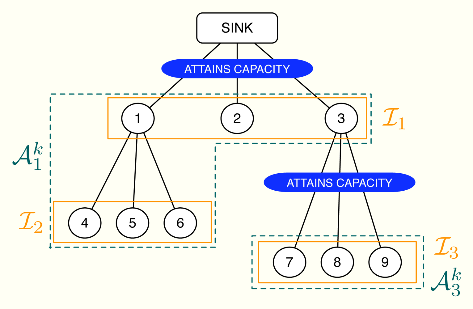
In the following, we assume that all the nodes in the network first make a rate request according to the amount of information they have to send. After running the distributed allocation algorithm, all of them get a certain transmission rate. The allocation depends on the rate requests, the priorities of the sensors, the minimum guaranteed rates and the maximum transmission rate at each level of the tree topology. All these parameters are known beforehand and the goal is to provide a fair rate distribution so that all the sensors in the network receive their transmission opportunities. On the contrary, note that a solution that maximizes the network throughput may prevent users with bad channel condition from transmitting. In practice, our solution is adequate for Frequency Division Multiple Access (FDMA) or Time Division Multiple Access (TDMA) since in both cases, it is possible to make an arbitrary division of the available total transmission rate in terms of bandwidth and time, respectively. Figure 1 provides a general view of our demand-based solution, where each dashed box represents one multiple-user communication channel between the parent node and its child nodes. Furthermore, a circle represents a node (sensor) and a line between two nodes simply indicates that they can communicate (using the corresponding multi-user channel).
2.1. Problem Formulation under Fairness Considerations
Let us consider the following optimization problem [16]
The optimization framework in Problem (1) is known to provide a fair distribution of resources if the utility functions Uj are adequately chosen [19,20]. Moreover, we can specify the desired degree of fairness by fixing the parameter γ in the following family of utility functions [21] (Lemma 2) in Equation (2). Furthermore, wj ∈ ℝ+ is defined as the priority of the j-th flow and it is used to balance the flow allocation towards the j-th sensor once the value of γ is fixed (the higher the value of wj, the larger the allocation).
In our WSN scenario, we assume that the network is built-up so that each sensor knows the route to the sink inside the cluster tree. Furthermore, each parent node has the information about the maximum transmission rate of its cluster, which is given by its own superframe configuration, and each sensor has evaluated its radio link quality, e.g., by means of the Packet Delivery Ratio (PDR). Given all this information, the goal is to compute a fair distribution of the available rate among the sensors. In the following, we focus our attention in the resolution of Problem (1) and we leave the practical implementation issues to Section 3. From the point of view of the optimization mechanism, note that one possibility is to gather all the requests at the sink node, compute there the optimal rate allocation and send it back to the sensors. Although there exist very efficient methods in the literature to solve generic convex problems, e.g., the so-called interior point methods [18] (Section 11.7), this approach is impractical in large-scale sensor networks as far as it implies an excess of signalling information. Therefore, there is a big interest in solving the problem as efficiently as possible, in a distributed manner. Efficient here means that: (i) the amount of signalling in the network and (ii) the computational load at the sensors must be kept small.
2.2. Existing Work
The problem we have formulated in Problem (1) is known in the literature as the Network Utility Maximization (NUM) problem [22] and several authors have employed classical decompositions, i.e., primal decomposition [17] (Section 6.4.2) and dual decomposition [17] (Section 6.4.1) to solve it. Dual decomposition is usually preferred since it naturally provides a full distributed solution [23,24]. Indeed, the Active Queue Management (AQM) policy employed in the Transport Control Protocol (TCP) can be viewed as a convex optimization problem that is distributedly solved using a dual decomposition approach. Notwithstanding, optimally solving Problem (1) in a distributed manner is now time and signalling consuming due to the fact that the algorithms are based in a projected subgradient approach [17] (Section 2.3). In general, the convergence of the algorithms is slow and furthermore, it depends on a user-adjusted step-size, which is not necessarily optimally fixed.
In order to overcome these drawbacks, we have proposed the Coupled-Decompositions Method (CDM) [11,12]. It simultaneously intertwines primal and dual decomposition techniques in a single approach, converges much faster to the optimal solution and avoids the choice of a user-defined step-size. Note that there exist other primal-dual convex methods in the literature that are different to our approach. Some of them do not take into account the separability of the problem and thus are not true decomposition-based techniques [25,26]. Other works use primal and dual domains as well as the separability of the problem but they concatenate primal and dual domains in their algorithms instead of really mixing them [22,27,28], as we do in our CDM. In the following, we briefly review the classical decomposition methods. Afterwards, we extend the formulation of the CDM to rate allocation problems that exhibit a tree topology thus obtaining a novel distributed version of the method.
2.3. Review of Primal and Dual Decompositions
Let us consider the following equivalent version of Problem (1), which contains the additional variables y = [y1, . . ., yN]T with y ∈ ℝN,
On the other hand, the primal master problem is defined as
Dual decomposition is the dual-domain version of primal decomposition and, in this occasion, we focus on the dual problem [18] (Section 5.2). In particular, we relax only the coupling constraint Ay ≼ c in Problem (3) thus defining the following dual master problem,
Taking into account that we consider cluster-tree WSNs in this paper, both primal and dual decompositions can be used to deploy distributed flow optimization solutions. However, these techniques suffer from convergence speed and the need of adjusting or , as discussed before. In the next subsection, we extend the authors’ proposed Coupled-Decompositions Method (CDM) [11,12] to provide a fully distributed solution in cluster-tree WSNs. Different to [11], we propose here a single stage algorithm where each iteration of the technique takes into account all the nodes. In [11], the proposed solution had several stages and in each stage, the nodes that belonged to the same network level were optimized thus involving several iterations. Therefore, the total number of iterations grew exponentially with the number of levels in the network. This drawback is overcome in the enhanced version of the method that we describe next.
2.4. Proposed Algorithm
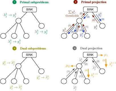
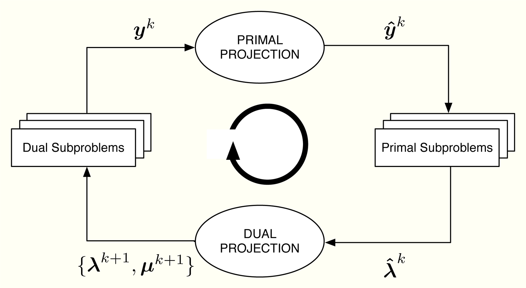
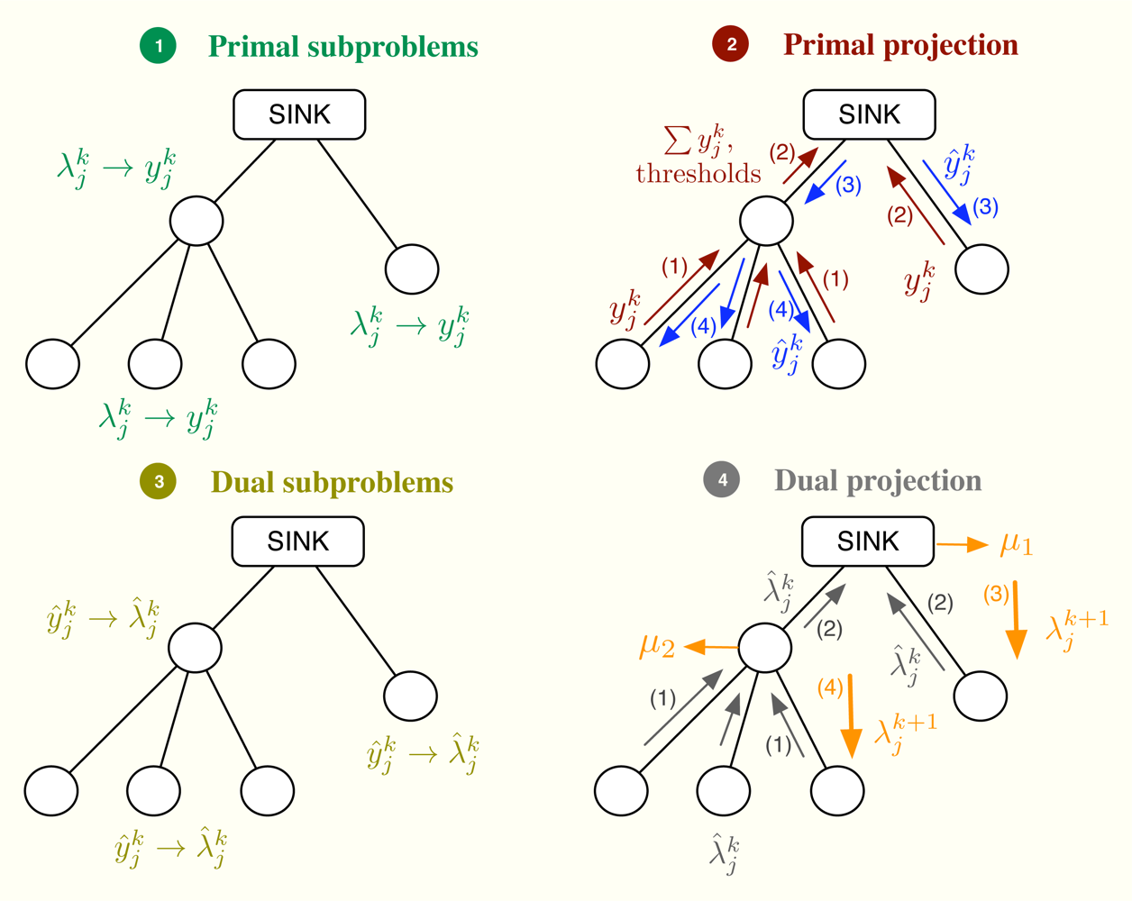
Let us consider the problem formulation in Problem (3) and let us define λj as the Lagrange multiplier (equivalently, dual variable) associated with the constraint rj ≤ yj for all j. As in dual decomposition, we keep μ = [μ1, . . ., μL]T as the multipliers associated with the constraints in Ay ≼ c. The technique we propose here intertwines primal and dual decompositions in a single approach and it is composed of four building blocks, namely: (i) dual subproblems; (ii) primal projection; (iii) primal subproblems and (iv) dual projection (see Figure 2). Before going to a more detailed description of the method, let us sketch out the four steps in the Figure 2, that form a complete iteration of the CDM, using a resource-price interpretation. From a practical point of view, this overview together with the contents of Section 2.5 shall suffice to develop our solution in real networks.
It is usual in convex optimization to think of primal variables as resources and dual variables as the prices to be paid for them. Let us assume that μk fixes, at time instant k, the cost of transmitting one unit of rate through each of the available multiple-user channels. Note that the more congested the channel, the higher the cost is and that the cost for a non-congested channel is 0. Given μk, each sensor obtains as the sum of the prices in the multiple-user channels it uses. When the sensor computes the dual subproblem from , it decides how many resources to buy, i.e., , which essentially depends on its own utility function. However, the overall rate acquisition may violate the constraints in the network and it must be corrected. This is the task of the primal projection, that is, it gathers all the values in and modifies them to in order to satisfy the network constraints. Thereafter, the primal subproblems estimate the price they will pay for the new allocation, i.e., . Finally, the dual projection looks at all the individual prices and tries to find a new consensus price μk+1. The entire process is repeated until all the sensors agree on the prices of the multiple-access channels.
Next, we describe one iteration of the method that starts with μk and ends up with μk+1. Afterwards, we prove in Section 2.8 that μk → μ*. In the following, a star as in y* or μ* indicates optimal values and a superindex k as in yk or μk indexes iterations. Furthermore, we make use of some of the Karush-Kuhn-Tucker optimality conditions [18] (Section 5.5.3) of Problem (3). These are
2.4.1. Dual Subproblems
From μk, each sensor computes as in Equation (10). Thereafter, the sensor solves the following optimization problem,
2.4.2. Primal Projection
In primal projection, the following optimization problem is solved,
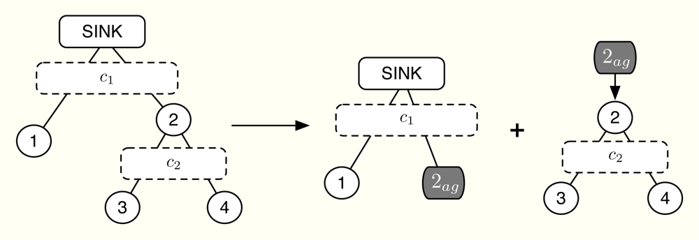
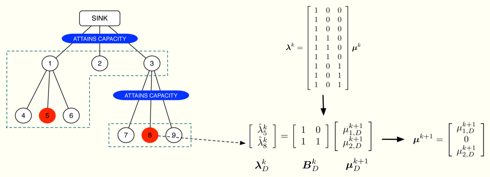
For the sake of brevity, we describe the distributed computation of Problem (14) using the example in Figure 3, which can be easily extended to the general case. Let us assume that [A]1 ŷ = c1 (this is usually the case) and [A]2 ŷ ≤ c2 [31]. For the sake of simplicity, we omit the index k in this example. As depicted in Figure 3, the idea is to compute the projection at the parent nodes, that is, first the sink allocates ŷ1 and ŷ2,ag and thereafter, sensor 2 allocates ŷ2,ag to sensors 3–4 and itself, thus obtaining ŷ2, ŷ3 and ŷ4. On the other hand, the application of the KKT optimality conditions to our simplified problem reveals us that the optimal solution must satisfy
In summary, the primal projection is distributedly found as follows. First, we compute the initial allocation with Equation (17). If , then we allocate ŷ2,ag to sensors 2–4 and we are done. If not, we allocate c1 − c2 to sensors 1–2 and c2 to sensors 3–4. Finally, this approach can be scaled to any tree-deployed sensor network. In general, a parent node has to signal at most ml 4-tuples, where ml is the number of network levels below it. Each 4-tuple contains an aggregated rate demand, the number of nodes involved in that demand, a threshold value and the rate absorbed once the allocation is above it. Note that this threshold value indicates the maximum possible allocation for a given hypothesis, that is, which channels are congested and which not. Therefore, the absorbed rate must correspond to this specific hypothesis. Once this information is available at the sink node, it can make the first-level allocation and successively, all parent nodes can compute their own allocations.
2.4.3. Primal Subproblems
Once the sensors receive the corrected allocation , they solve the following optimization problem,
2.4.4. Dual Projection
The dual projection is the last step of the method and its mission is to update μ having the information in λ̂k. We already know that one of the optimality conditions of our problem is Equation (10). However, this linear system of equations is in general overdetermined and we can not use it to guess μk+1 from λ̂k. Fortunately, it is possible to choose some of the entries in λ̂k to obtain an alternative system of equations, say , that determines the non-zero values in μk+1. Note that due to Equation (11), is necessarily 0 if the corrected allocation after the primal projection verifies [A]jŷk − cj < 0. In the following, we describe how and are constructed.
First of all, let us define the subsets of nodes m and . The subset m does not depend on the iteration number and includes all the nodes using the m-th wireless channel except for the parent node. On the contrary, depends on the subset of active constraints [32] in the network, which evolves on time. Specifically, if the n-th channel is congested, the subset is the union of n with all the subsets m that accomplish: (i) the path from any of the nodes in m to the sink goes through one of the nodes in n and (ii) none of these paths makes use a congested channel, that is, the channels in the path do not attain their rate constraints with equality. If the n-th channel is not congested, we do not define . A simple example can be found in Figure 4, where 1 = {1, 2, 3}, 2 = {4, 5, 6} and 3 = {7, 8, 9}. In this example, we transmit at the maximum possible rate only in channels 1 and 3 whereas channel 2 is not congested. Therefore, we define and but not 𝒜2.
Once the subsets { } are identified, we select one sensor from each group using the following selection rules:
(SR1) Choose the node with the value of that is closest to (note that if i, ) and that verifies (SR2).
(SR1) The corresponding value in attains (as shown in Proposition 3, there is at least one value of inside the interval).
The proposed solution has two phases. The first phase begins at the lowest levels of the cluster-tree and each node sends its current value of to its parent. The parent, in turn, first checks if the channel with its child nodes is congested. If true, it sends its own value of . If false, it takes the values from the child nodes and also its own value and selects one candidate according to (SR1)-(SR2). This is the value that is sent to the parent in this second case. This process is successively applied until the sink node is reached. Thereafter, the second phase begins. The sink node checks if it attains its own rate constraint. If true, it selects one value taking into account (SR1)-(SR2), fixes μ1 to that value and sends it to its child nodes. If false, it fixes μ1 = 0 and sends it. When the child nodes receive that value, say vi, select one among its gathered values using again (SR1)-(SR2) and compute μi (the dual multiplier associated with its rate constraint) as . If the resulting μi ≥ 0, the parent node sends to its child nodes; if μi < 0 or if the channel between the node and its children is not congested, the parent fixes μi = 0 and sends the received vi to its child nodes. This process is repeated until all the values in μk+1 are updated. Note that, as a result of the proposed distributed dual projection, each parent node only knows one value in μk+1 but each node receives its own so that the next iteration of the method can begin.
Finally, we have to decide when to stop the iterations of the CDM, that is, when the current solution is close enough to the optimum. One possibility is to monitor the distance between yk and ŷk and to stop when the relative distance between both quantities drops below a predefined value ε, that is, when
2.5. Algorithmic Form
The CDM can be summarized in algorithmic form as follows:

| Start with k = 0, μ0 = 0 and repeat: |
| Dual Subproblems |
| 1⃞ Using
, compute
and get as the inner maximizer. |
| Primal Projection |
| 2⃞ Solve
distributedly as sketched in Section 2.4 in order to get . |
| Primal Subproblems |
| 3⃞ Solve
and get as the dual multiplier associated with the constraint . |
| Dual Projection |
4⃞ Phase I. The lowest level nodes send
to their parents. Then repeat:
Until the sink node has received one value of from each of its child nodes. Phase II. Start at the sink node with v1 = 0 and repeat:
Until all the values in μk are determined and all the values in λk are updated to λk+1. |
| Until convergence. |
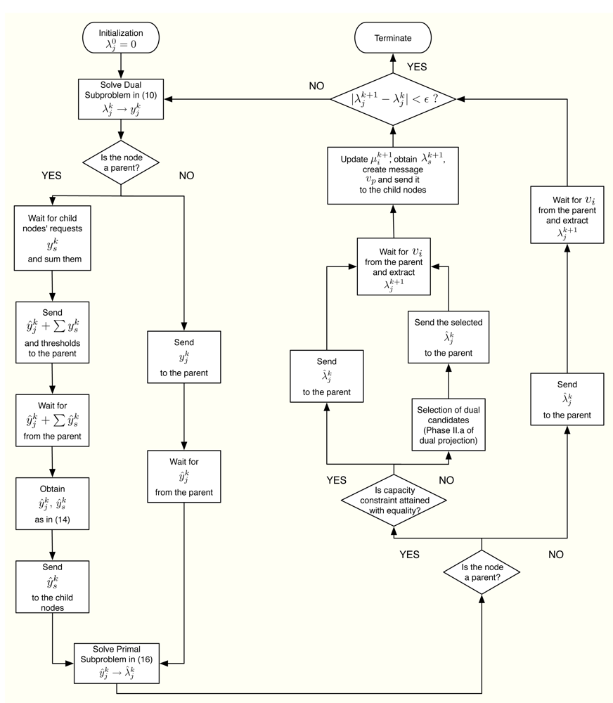
Furthermore, Figure 6 summarizes in a flowchart all the tasks that a sensor has to execute in order to obtain its optimal rate allocation.
2.6. Signalling in the Coupled-Decompositions Method
In distributed implementations such as the one proposed in this paper, signalling plays a crucial role. In the following, we review a complete iteration of the proposed method from the point of view of signalling and we represent it graphically in Figure 7. Let us assume that at the k-th iteration, all the nodes know the values of and use them to compute the dual subproblems. As a result, they locally obtain the values of involving no signalling. Thereafter, in primal projection, the parent nodes must send their aggregated request , i.e., the sum of the values that belong to their subtree, possibly together with a list that includes allocation threshold values and absorbed rates, as discussed in Equations (17) and (18). Note that the size of the list scales linearly with the number of levels in the subtree. Once the request reaches the sink node, it allocates resources to the first level of the tree. In turn, the nodes at the first level allocate their resources to the nodes at the second level and so forth. When all the nodes have received the corresponding value , they locally compute the primal subproblems and obtain the values . Finally, in order to compute the dual projection, the nodes send the values to their parent nodes. Thereafter, the sink node computes μ1 and broadcasts the value to their child nodes (note that all the child nodes receive the same value). In turn, the parent nodes compute their own value μj and broadcast to their child nodes. This process is successively applied until all the nodes receive the updated value of the dual variable, which completes one iteration of the proposed CDM.
2.7. Differences with Classical Decompositions
From the point of view of the algorithm, two of the building blocks in the proposed method are the same as in the classical decompositions, that is, the definition of the primal and the dual subproblems has not been modified. On the contrary, the primal and the dual projections differ from the primal and dual master problems as far as subgradients are no longer used. Notwithstanding, the primal projection resembles the projection that appears in the primal master problem. The difference is that we force the constraints in Ay ≼ c to be attained with equality when the corresponding dual variable in μ is not zero. Finally, the dual projection is completely different from the master dual problem and is indeed the key block in our proposal.
From the point of view of signalling, one iteration in traditional primal decomposition algorithms is equivalent to the first two steps in the proposed method. In other words, from the nodes compute the primal subproblems and calculate , which requires no signalling. Thereafter, the projection [·]† in traditional primal decomposition algorithms requires the same amount of signalling as in the worst-case of the primal projection at the CDM, that is, when [A]jy ≼ cj, ∀j. Similarly, one iteration in the traditional dual decomposition is equivalent to the last two steps of the CDM. That is, from μk, the nodes implementing the traditional dual decomposition approach obtain , which requires no signalling, and afterwards send these values to the parent nodes. Using that information the parent nodes can extract the values of μk+1 and send the required linear combination of the values in μk+1 back to the child nodes. In this case, the total amount of signalling is exactly the same as in the dual projection of the CDM, where the nodes send the current allocation, the parent nodes compute the required subgradient and send the updates of the values in λ afterwards.
In summary, the key step that allows us to combine traditional primal and dual decompositions in a single algorithm, the CDM, is the dual projection. Conceptually, the big difference is to interpret the primal variables yk, ŷk and the dual variables λk, λ̂k as candidates to the optimal solution that must accomplish the well-known KKT optimality conditions. In terms of signalling, one iteration of the CDM is equivalent to two iterations of the traditional decomposition algorithms.
2.8. Convergence to the Optimal Rate Allocation
Let us start the iterations of the proposed CDM with μ0 = 0. In the following we show that μk → μ* as k increases. Initially, we assume that at the k-th iteration only if , that is, the active constraints (i.e., attained with equality) at the k-th iteration are exactly the same as in the optimal solution and we prove that the algorithm converges to μ*. Afterwards, we describe the mechanism used by the CDM in order to activate or deactivate constraints until the subset of active constraints in the optimal solution is found out.
Convergence to the Optimal Solution Given the Subset of Active Constraints at the Optimum
Let us first recall in Proposition 1, a known result that establishes the relationship between primal and dual variables in the primal and dual subproblems [11,12].
Proposition 1 Let us consider the j-th primal subproblem in Problem (19) and the j-th dual subproblem in Problem (13) of the CDM. Then, the inner optimization variable is a decreasing function of in the primal subproblems and the inner optimization variable is a decreasing function of in the dual subproblems.
Proof See [12] (Lemma 2).
Note, in particular, that if as a result of the primal subproblems, then it is true that and vice versa. Similarly, if as a result of the dual subproblems, then and vice versa. Note also that given μk, all the values with j ∈ i attain either or as far as [AT]j is exactly the same for all j ∈ i. That is, if we start an iteration of the CDM with λk in the dual subproblems, it holds that for all j ∈ k if and vice versa due to Proposition 1.
Once we obtain the values yk from the dual subproblems, the primal projection in Problem (14) is computed. Since we assume that Slater’s condition holds, Problem (14) defines a convex program where strong duality is fulfilled. Therefore, KKT optimality conditions can be applied and the solution to the primal projection can be expressed as
In that situation and given the tree structure of the network, it is verified that
Proposition 2 The dual values that result from the computation of the primal subproblems of the CDM at the k-th iteration accomplish: (i) some values of with attain while the rest accomplish and (ii) all the values with either increase or decrease with respect to (note that if l,).
In the dual projection, we choose one value from each subset . In particular, the selected value has to accomplish (SR1)-(SR2), that is: (i) the corresponding verifies and (ii) it is the closest value in the subset to for any . The following proposition guarantees the existence of the required value.
Proposition 3 Let yk be the result of the dual subproblems of the CDM at the k-th iteration. Then, the primal projection provides at least one node with at each subset.
Proof See the Appendix.
Given that Uj(rj) is concave and strictly increasing, it is straightforward to see that yj must equal rj in Problem (3). Furthermore, some of the KKT optimality conditions of the problem reveal us that
Finally, in the dual projection we construct the determined linear system with the selected values , thus computing the values in μk+1 corresponding to the active constraints (the remaining ones are fixed to zero). Combining the results in Proposition 2 with (SR1)-(SR2), we realize that each dual candidate approaches (w.r.t. ) without overtaking it and that the candidate is valid to determine some of the variables in μk+1. Since in the dual projection we obtain a determined linear system using these dual candidates, the new update λk+1 = [A]T μk+1 necessarily approaches λk = [A]T μk. Hence, we can state that μk → μ*. We summarize this result in the following lemma.
Lemma 1 The iterations of the CDM satisfy given the subset of active constrains at the optimum.
Activation/Deactivation of Constraints
In the following, we use the partial result obtained in Lemma 1 to show that the proposed version of the CDM converges to the optimal solution. Let us state this in the following theorem.
Theorem 1 The proposed CDM is able to determine the subset of active constraints of Problem (3) at the optimal solution. Hence, the method converges to the optimal solution.
Proof We have proved in Lemma 1 that, given the subset of active constraints at the optimum, the CDM converges to μ*. Therefore, we need to prove that this subset is eventually found out. Let us start with the activation of a non-active constraint and let us assume that the l-th constraint is active at the optimal solution but not at the k-th iteration. This implies that, if we remove the constraint [A]ly ≤ cl from the original problem formulation in Problem (3), then the optimal solution to the modified problem y‡ would satisfy [A]ly‡ ≥ cl. In other words, the successive updates of the CDM tend to y‡ when the l-th constraint is not included in the active subset of constraints. However, there will be an iteration q where [A]lyq ≥ cl so that the primal projection will detect that constraint violation, correct it and the l-th constraint will be activated.
The opposite situation arises when the l-th constraint is active at the k-th iteration but not at the optimal solution. In that case, if the l-th constraint is not deactivated, i.e., the primal projection keeps forcing Ay = cl, the CDM would converge to a solution μ★ with (assuming that the dual projection allows negative values). Note that the allocation to the variables involved in the l-th constraint increases with respect to the optimum whereas the allocation to the remaining variables is reduced or remains unchanged in order to satisfy the rate constraints. Looking at the situation from the dual point of view, that is, taking into account Proposition 1, we notice that the values involved in the l-th constraint must converge to a value that is below . Also, the remaining values remain unchanged or above the corresponding . If we compare those values with λ* = AT μ* and we know that , then we realize that . At this point, let us compute one more iteration of the CDM, thus obtaining λ★+1. In this case, since the values involved in the l-th constraint increase with respect to λ★ = AT μ★ because is now 0, the corresponding values decrease. Therefore the l-th rate constraint will not be exceeded, preventing its reactivation at the next primal projection.
3. Application to Cluster-Tree Wireless Sensor Networks
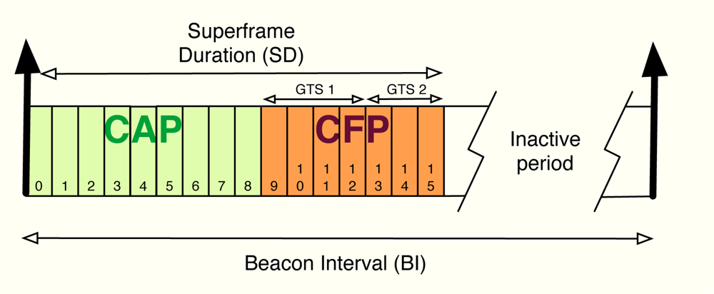
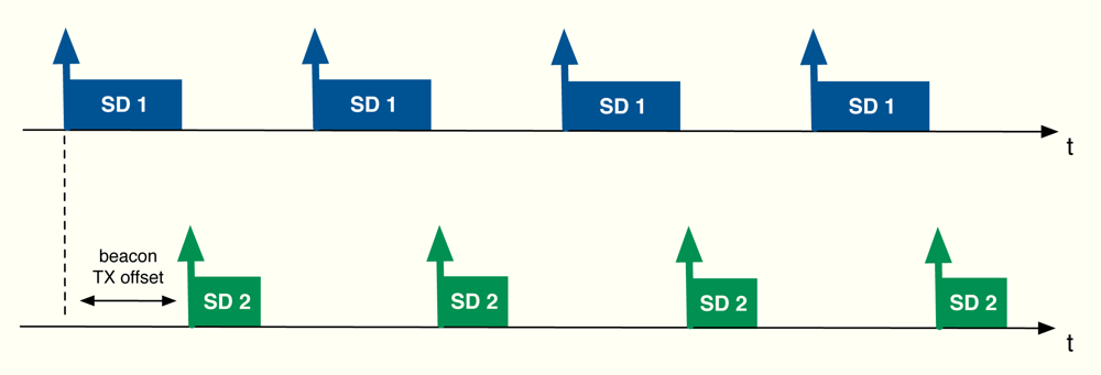
The algorithm developed in the previous section can be applied to cluster-tree WSNs with the aim of providing global fair resource allocations with a reduced impact in terms of energy consumption due to signalling. In this work, in particular, we focus on the beacon-enabled mode of IEEE 802.15.4 [1]. This mode divides the transmission through time slots and, besides, two periods are defined depending on the kind of access used by the nodes in the network: contention access period (CAP), where slotted CSMA/CA is adopted, and contention-free period (CFP), where GTS slots are distributed to the nodes (see Figure 8). Since time slots can have different sizes from one cluster to another, we distribute resources in terms of rate, i.e., rj is the rate allocated to the j-th sensor. Thereafter, we use these rates to derive the time slot allocation. Note that depending on each specific Superframe (SF) configuration, the maximum transmission rate in each cluster changes. Furthermore, we will also take into account the quality of the radio links by means of the Packet Delivery Ratio (PDR), that is, PDRj is the ratio between correctly received packets and sent packets at the j-th sensor. As previously commented, beacon collision problems can appear in a cluster-tree WSN based on the beacon enabled mode. For that reason, we take into account a beacon collision mechanism. In particular, we consider the time-division approach adopted by the Zigbee specification [9], i.e., time is divided in such a way that the beacon frame of each coordinator is sent during the inactive periods of the rest of coordinators (see Figure 9).
Given the sensor demands in M = [M1, . . ., MN ]T and the minimum guaranteed allocation in m= [m1, . . ., mN ]T (both in terms of rate), the optimum allocation is computed by solving the following optimization problem using the CDM,
Once the optimal allocation is obtained, it has to be mapped onto a time slot assignment. Since the WSN scenario can be assumed quasi-static in most of the real-life applications, it is reasonable to sustain an allocation for a given number of Beacon Intervals (BI), say nBI. Therefore, the real-valued number of time slots assigned to the j-th sensor on the nBI periods is
4. Numerical Results
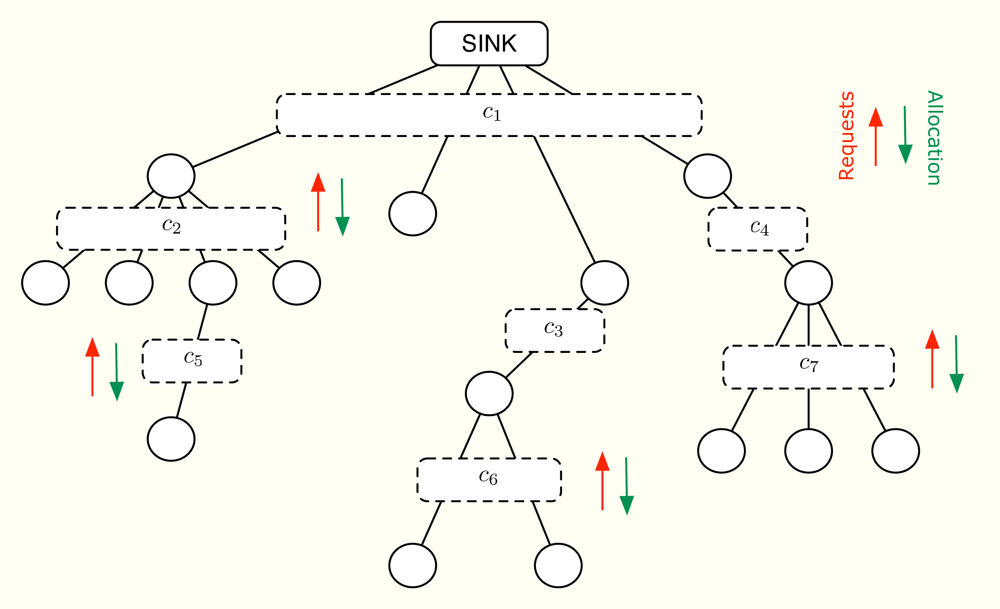
Let us consider the network configuration depicted in Figure 10, with 15 sensor nodes, one sink node and 5 capacity constraints that deploy a three-level cluster tree. Note that the following results can be extrapolated to WSNs with a larger number of nodes and a larger number of levels and thus, our simplified example has no loss in generality. Specifically, the Superframe (SF) is configured as follows: TBI is set to 245.76 ms and is the same at all levels; the SF duration is 61.44 ms at the highest level, 30.72 ms at the intermediate level and 15.36 ms at the lowest level. According to [33], this configuration provides 9.38 kbps, 10.94 kbps and 13.02 kbps of data rate, respectively. Furthermore, if we consider 15 slots per BI dedicated to the Guaranteed Time Slot (GTS) allocation, the size of the slots in bits is 9, 21 and 50, respectively. Accordingly, the rate capacities of the clusters are set to c = [3.0516, 1.2820, 1.2820, 1.2820, 0.5496]T kbps.
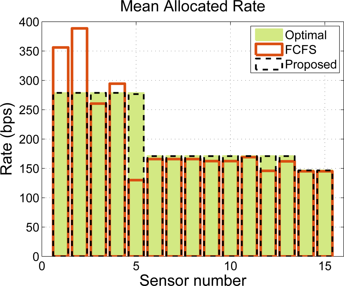
In our simulations, we compare our CDM-based approach to the widely-used First Come First Serve (FCFS) policy. We assume, without loss of generality, that the values of wj and P DRj are set to 1 and that all the sensors are of the same type and thus, all of them need to transmit n bits per BI. However, the rate requests are quantized by the time slot duration at each sensor so that each node asks for n̄i/TBI kbps, where n̄i is the nearest multiple (above) of the packet size in bits at the i-th node. Figure 11 shows an allocation example for n = 20 bits. We notice that the CDM-based policy provides a rate allocation that is very close to the optimal, whereas the FCFS solution does not guarantee a fair resource allocation, even when the throughput is not penalized. Note that, in the example under consideration, there exists no trade-off between fairness and throughput because we have set error-free links. Note also that our proposed time slot allocation does not provide the optimum fair rate allocation due to the rounding effects.
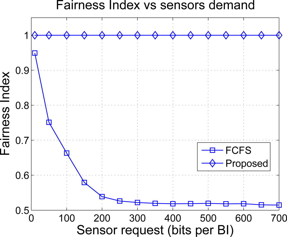
In order to study the fairness degree provided by both solutions, we plot in Figure 12 the Fairness Index (FI) as a function of the requested bits n. The FI takes values between 0 and 1 and measures how far is a certain resource allocation with respect to the one that is considered optimal or most fair. If FI = 0 the allocation is totally unfair and if FI = 1, the resulting allocation is completely fair. A value that is in-between such as 0.6 may be interpreted as follows: the 60% of allocations are considered fair in mean. The FI is computed as [34]
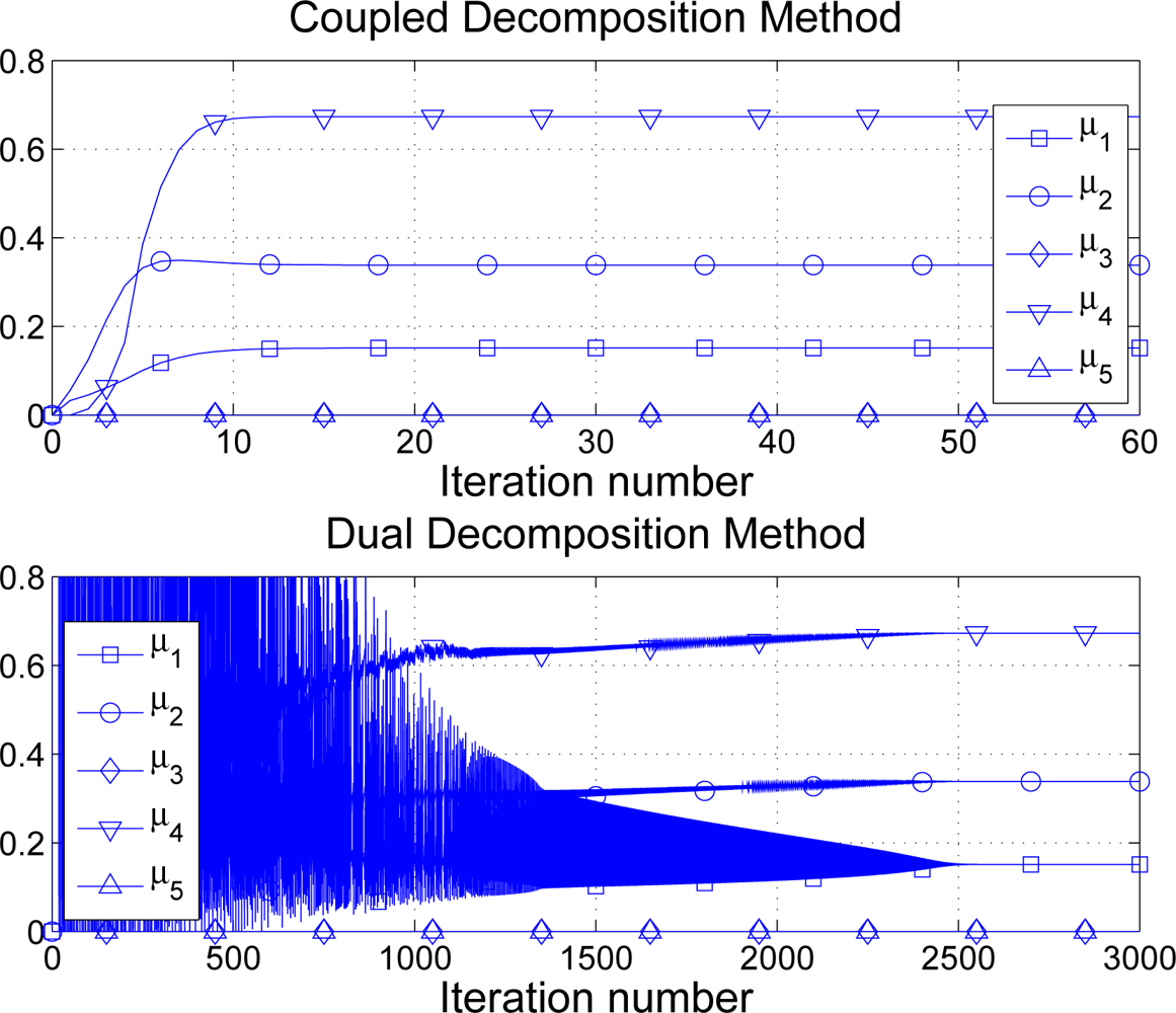
Finally, signalling is a very important aspect to take into account when considering distributed optimization techniques. The advantage is clear: the network operates at the desired optimal point (proportional fairness in our examples). Notwithstanding, as opposite to other policies such as FCFS, sensors need to exchange information thus draining the sensor batteries. Therefore, distributed optimization approaches make sense if the amount of signalling information is kept small. In Figure 13 we compare the proposed CDM against the classical dual decomposition approach in terms of iterations required to converge to the optimal solution. In this example, requests, maximum transmission rates, minimum guaranteed rates and sensor priorities are picked at random using uniform distributions. In particular, di, ci ∼ [0, 50] kbps, mi ∼ [0, 0.5] kbps and pi ∼ [0, 2]. In our simulations, the step-size in dual decomposition is adjusted to provide good performance in general, fixing it to (note that the CDM has no parameter to configure). See in Figure 13 one numerical example. Note that although one iteration of the CDM implies twice the amount of signalling required in one iteration of dual decomposition, the number of iterations in the latter is excessively large and makes the technique impractical in the WSN context. On the contrary, the CDM finds the optimal solution using 10–30 iterations in general. In other words, the CDM requires about 40 N to 120 N messages to achieve a fair distribution of the available rate whereas the so-called dual decomposition solution needs to exchange up to 5, 000 N in our example. If we consider 32-bit messages, our solution requires 56.25 kb in total whereas the dual decomposition approach needs 2343.75 kb of signalling.
5. Conclusions
In this paper, we present a resource allocation technique that is designed to fairly distribute the available time slots among the sensors of a cluster-tree WSN. Our solution is based in convex decomposition and, in particular, it combines the so-called primal and dual decompositions in a single algorithm that provides superior performance in terms of convergence speed. Thanks to the proposed Network Utility Maximization (NUM) formulation, it is possible to choose the most adequate definition of fairness in our application, going from max-min fairness to max-sum rate. As shown in the document, the standard-proposed First Come First Serve policy provides pretty unfair allocations when the traffic load in the network increases and proportional fairness is considered. Moreover, the NUM formulation takes into account the different rate capacities in the network, which are due to different superframe configurations, as well as the radio link qualities by means of the Packet Delivery Ratio.
Throughout the document, we focus our attention on the practical application of the proposed method. On one hand, the conversion form rate (required by the algorithm) to time slots is addressed. On the other hand, the signalling involved in the computation of the global optimal solution is detailed. Specifically, our method requires the double amount of signalling per iteration when compared to dual decomposition. Notwithstanding, the number of iterations can be reduced up to a factor of 1,000 so that the total amount of signalling is reduced about 500 times. Besides, the CDM has no parameter to be adjusted, which is a true impairment in practice.
In summary, we can conclude that the most remarkable benefits of our solution are:
The network can be adjusted to operate with several fairness definitions by fixing the value of γ.
The optimal solution is distributedly computed in the cluster-tree network.
The price to pay to compute that optimal solution in terms of signalling is minimized with respect to existing techniques.
Acknowledgments
This work was supported by the Spanish Government Project TEC2008-06305/TEC, the Catalan Government under Grant 2009 SGR 298, and the Chair of Knowledge and Technology Transfer Parc de Recerca UAB—Santander. I.V. is partially funded by Torres Quevedo grant from the Ministerio de Ciencia e Innovación 2008-03-08109. We are also grateful to the HAROSA Knowledge Community ( http://dpcs.uoc.edu/) and to FP7-IAPP-SWAP EU contract number 251557 that partially funded our research.
References and Notes
- IEEE. Wireless Medium Access Control (MAC) and Physical Layer (PHY) Specifications for Low-Rate Wireless Personal Area Networks (LR-WPANs); IEEE Std 802.15.4; IEEE: New York, NY, USA, 2006. [Google Scholar]
- Koubaa, A; Alves, M; Tovar, E. IEEE 802.15.4 for Wireless Sensor Networks: A Technical Overview; IPP-HURRAY Technical Report; HURRAY-TR-050702; Polytechnic Institute of Porto: Porto, Portugal, 2005. [Google Scholar]
- Chen, F; German, R; Dressler, F. Towards IEEE 802.15.4e: A Study of Performance Aspects. Proceedings of 8th IEEE PERCOM, Mannheim, Germany, 29 March–2 April 2010.
- Kim, A; Hekland, F; Petersen, S; Doyle, P. When HART Goes Wireless: Understanding and Implementing the WirelessHART Standard. Proceedings of IEEE ETFA, Hamburg, Germany, 15–18 September 2008.
- ISA. Wireless Systems for Industrial Automation: Process Control and Related Applications; ISA: Research Triangle Park, NC, USA, 2009. [Google Scholar]
- Mishra, A; Chewoo, N; Rosenburgh, D. On Scheduling Guaranteed Time Slots for Time Sensitive Transactions in IEEE 802.15.4 Networks. Proceedings of IEEE MILCOM, Orlando, FL, USA, 29–31 October 2007.
- Chitnis, M; Pagano, P; Lipari, G; Liang, Y. A Survey on Bandwidth Resource Allocation and Scheduling in Wireless Sensor Networks. Proceedings of IEEE International Conference on Network-Based Information Systems, Indianapolis, IN, USA, 19–21 August 2009.
- IEEE 802.15 WPAN™ Task Group 4b. Available online: http://grouper.ieee.org/groups/802/15/pub/TG4b.html (accessed on 21 March 2011).
- Zigbee-Alliance. ZigBee Specification. Available online: http://www.zigbee.org (accessed on 21 March 2011).
- Koubaa, A; Alves, M; Attia, M; Van Nieuwenhuyse, A. Collision-Free Beacon Scheduling Mechanisms for IEEE 802.15.4/Zigbee Cluster-Tree Wireless Sensor Networks. Proceedings of 7th International Workshop on Applications and Services in Wireless Networks, Santander, Spain, 24–25 May 2007.
- Morell, A; Seco-Granados, G; Vicario, J. Fair Adaptive Bandwidth and Subchannel Allocation in the WiMAX Uplink. EURASIP J Wireless Communications and Networking 2009. [Google Scholar] [CrossRef]
- Morell, A. A Convex Decomposition Perspective on Dynamic Bandwidth Allocation and Applications, Ph.D. Thesis,. 2008. Available online: http://spcomnav.uab.es (accessed on 21 March 2011).
- The ROLL Design Team. RPL: Routing Protocol for Low Power and Lossy Networks (work in progress). 2010. Available online: http://tools.ietf.org/html/draft-ietf-roll-rpl-17 (accessed on 21 March 2011). [Google Scholar]
- Gnawali, O; Fonseca, R; Jamieson, K; Moss, D; Levis, P. The Collection Tree Protocol (CTP). Proceedings of 7th ACM Conference on Embedded Networked Sensor Systems (SenSys), Berkeley, CA, USA, 4–6 November 2009.
- Vilajosana, X; Llosa, J; Pacho, J; Vilajosana, I; Juan, AA; Vicario, J; Morell, A. ZERO: Probabilistic Routing for Deploy and Forget Wireless Sensor Networks. Sensors 2010, 10, 8920–8937. [Google Scholar]
- Notation: ≼, ≺,≽ and ≺ stand for component-wise inequalities.
- Bertsekas, D. Nonlinear Programming; Athena Scientific: Belmont, MA, USA, 1999. [Google Scholar]
- Boyd, L; Vandenberghe, S. Convex Optimization; Cambridge University Press: Cmbridge, UK, 2004. [Google Scholar]
- Kelly, F. Charging and Rate Control for Elastic Traffic. Eur. Trans. Telecommun 1997, 8, 33–37. [Google Scholar]
- Kelly, F; Maulloo, A; Tan, D. Rate Control for Communication Networks: Shadow Prices, Proportional Fairness and Stability. J. Oper. Res. Soc 1998, 49, 237–252. [Google Scholar]
- Mo, J; Walrand, J. Fair End-to-End Window-based Congestion Control. IEEE/ACM Trans. Netw 2000, 8, 556–567. [Google Scholar]
- Palomar, D; Chiang, M. Alternative Decompositions for Distributed Maximization of Network Utility: Framework and Applications. IEEE Trans. Autom. Control 2007, 52, 2254–2269. [Google Scholar]
- Xiao, L; Johansson, M; Boyd, S. Simulatenous Routing and Resource Allocation via Dual Decomposition. IEEE Trans. Commun 2004, 52, 1136–1144. [Google Scholar]
- Lee, J; Chiang, M; Calderbank, A. Network Utility Maximization and Price-Based Distributed Algorithms for Rate-Reliability Tradeoff. Proceedings of IEEE Infocom, Barcelona, Spain, 23–29 April 2006.
- Tseng, P; Bertsekas, D. On the Convergence of the Exponential Multipliers Method for Convex Programming. Math. Program 1993, 60, 1–19. [Google Scholar]
- Polyak, R. Primal-Dual Exterior Point Method for Convex Optimization. Optim. Method. Softw 2008, 23, 141–160. [Google Scholar]
- Holmberg, K. Primal and Dual Decomposition as Organizational Design: Price and/or Resource Directive Decomposition. In Design Models for Hierarchical Organizations: Computation, Information, and Decentralization; Kluwer Academic Publishers: Boston, MA, USA, 1995; pp. 61–92. [Google Scholar]
- Nedic, A; Ozdaglar, A. Subgradient Methods for Saddle-Point Problems. JOTA 2009, 142, 205–228. [Google Scholar]
- The vector s is a subgradient of the function f: ℝn → ℝ at x ∈ ℝn if f(y) ≥ f(x) + (y − x)T s, ∀y ∈ ℝn. If f is differentiable at x, the subgradient s and the gradient ∇f(x) coincide. Otherwise, there exist many subgradients.
- Notation: δj is a zero-valued column vector with its j-th entry equal to 1.
- Note that in the case [A]2ŷ = c2, Problem (14) is splitted into 2 independent projections: (i) distribute c2 between sensors 3 and 4 and (ii) distribute c1 − c2 between sensors 1 and 2.
- We say that a constraint is active when it is attained with equality.
- Koubaa, A; Alves, M; Tovar, E. GTS Allocation Analysis in IEEE 802.15.4 for Real-Time Wireless Sensor Networks. Proceedings of Parallel and Distributed Processing Symposium (IPDPS), Rhodes Island, Greece, 25–29 April 2006.
- Jain, R; Chiu, D; Hawe, W. A Quantitative Measure of Fairness and Discrimination for Resource Allocation in Shared Systems; Technical Report; DEC TR-301; Digital Equipment Corp.: Littleton, MA, USA, 1984. [Google Scholar]
Appendix
Proof of Proposition 3
As it is discussed after Problem (21), the step from yk to ŷk forces all the values in each subset to either increase or decrease their allocation in order to fulfill the corresponding rate constraint. Let us consider the first case, i.e., all the values of with satisfy . Since , it is straightforward to see that . However, it is possible that . Notwithstanding, this implies that there is no strictly feasible point in the original problem, which contradicts the initial hypothesis. Note that we need to increase all the values in to reach a strictly feasible point but this violates the rate constraint. Therefore, there is at least one value that accomplishes .
Similarly, we can consider the second case, that is, the values of with are increased in the primal projection. In this occasion, if the resulting point verifies , it implies that the associated constraint is not really necessary. However, this contradicts our hypothesis that the subset of active constraints at the optimum is known. This concludes the proof of the proposition.


© 2011 by the authors; licensee MDPI, Basel, Switzerland. This article is an open access article distributed under the terms and conditions of the Creative Commons Attribution license (http://creativecommons.org/licenses/by/3.0/).
Share and Cite
Morell, A.; Vicario, J.L.; Vilajosana, X.; Vilajosana, I.; Seco-Granados, G. Optimal Rate Allocation in Cluster-Tree WSNs. Sensors 2011, 11, 3611-3639. https://doi.org/10.3390/s110403611
Morell A, Vicario JL, Vilajosana X, Vilajosana I, Seco-Granados G. Optimal Rate Allocation in Cluster-Tree WSNs. Sensors. 2011; 11(4):3611-3639. https://doi.org/10.3390/s110403611
Chicago/Turabian StyleMorell, Antoni, Jose Lopez Vicario, Xavier Vilajosana, Ignasi Vilajosana, and Gonzalo Seco-Granados. 2011. "Optimal Rate Allocation in Cluster-Tree WSNs" Sensors 11, no. 4: 3611-3639. https://doi.org/10.3390/s110403611