Modeling the Behavior of an Underwater Acoustic Relative Positioning System Based on Complementary Set of Sequences

 ,
,
Abstract
: The great variability usually found in underwater media makes modeling a challenging task, but helpful for better understanding or predicting the performance of future deployed systems. In this work, an underwater acoustic propagation model is presented. This model obtains the multipath structure by means of the ray tracing technique. Using this model, the behavior of a relative positioning system is presented. One of the main advantages of relative positioning systems is that only the distances between all the buoys are needed to obtain their positions. In order to obtain the distances, the propagation times of acoustic signals coded by Complementary Set of Sequences (CSS) are used. In this case, the arrival instants are obtained by means of correlation processes. The distances are then used to obtain the position of the buoys by means of the Multidimensional Scaling Technique (MDS). As an early example of an application using this relative positioning system, a tracking of the position of the buoys at different times is performed. With this tracking, the surface current of a particular region could be studied. The performance of the system is evaluated in terms of the distance from the real position to the estimated one.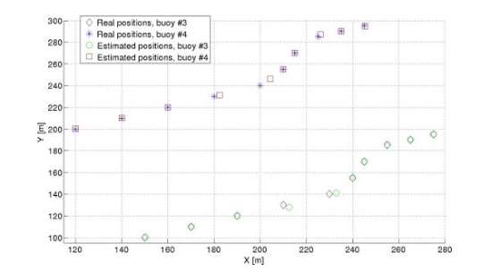
1. Introduction
All systems need a good understanding of the medium in which they are deployed. Particularly, underwater medium is highly dynamic and difficult to model due to some effects as swell, turbulences or the irregular spatial distribution. Nevertheless, a propagation model is needed to test the behavior of any system prior its actual deployment. Until now, a large number of models have been proposed, based on different mathematical approaches such as ray tracing, normal mode or the parabolic equation, to name a few, where their use is suggested for different scenarios or purposes.
Ray tracing provides an intuitive approach to acoustic propagation, assuming that the energy of the wave is confined in different paths, allowing to think in rays rather than waves. This is a good assumption if the amplitude of the wave and sound speed do not change noticeably in a wavelength. Through all these years, several ray tracing codes have been developed [1–3]. These models are usually fast to compute, allow to set up the directionality of the source and can handle range-dependent sound speed profiles and bathymetry. On the other hand, they have problems with diffraction and caustics, so they are not so effective for studying bottom interactions and low frequency propagations [4].
Normal mode models are based on the integral representation of the wave equation, and provide the sound field as a sum of normal modes. They can compute transmission loss easily for a given combination of frequency, source depth, receiver depth and ranges, but they are range independent and the number of modes to compute depend on frequency, so they are recommended for frequencies below 500 Hz [5], unless more assumptions are considered on the environment. Two examples of these models are SUPERSNAP [4] and COUPLE, which uses coupled modes [6] to deal with range dependence.
Fast field theory is very similar to normal mode, but it uses an asymptotic expansion on the equation for the acoustic pressure field. The resulting infinite integral is evaluated by means of a fast Fourier transform and includes a branch line integral term that is usually neglected in normal modes [5]. Probably, the most famous fast field program is SAFARI [7], which can handle multiple sources and obtains the solution for all depths simultaneously, although it is not easy to use and the computation time can be very long.
Finite elements models divide the medium into a mesh. The length of the sides of this mesh is usually one tenth of the wavelength, and they intersect at nodal points. The wave equation is replaced by a system of algebraic equations, that can be solved to obtain the field at each node in the mesh. Because of that, a large computation time is required for long range and high frequency configurations [4]. There are few models based exclusively on this technique. However, it can be combined with other techniques, such as boundary integrals and wavenumber integration to solve the Helmholtz equation in a range-dependent ocean environment [8].
Other approach is the finite-difference time-domain, where a discretization of the time dependent curl equations of Maxwell is performed, and the wave propagation is simulated in the time domain. The feasibility on underwater acoustics problems was introduced in [9] using a finite-difference approximation of the Helmholtz equation, and in [10] was used for a scattering problem in an underwater medium. The Helmholtz equation can also be transformed into a boundary integral equation, and then a boundary element approximation can be used to solve it [11]. In [12], a model using the boundary element method is used to study the wave propagation in a environment with a bottom irregularity in a 3D environment.
The last main technique for modeling underwater acoustic propagation is the parabolic equation. This is an approximation of the elliptic Helmholtz equation, introduced in underwater acoustics in 1973 [4]. They can handle range dependent environments, but only narrow angles are valid, due to the approximation considered, computation time increases rapidly with signal frequency and they did not consider shear waves. Two examples of parabolic equation models are PAREQ, which dates back until 1975, and RAMS [13].
Whereas underwater modeling has been an active field since decades ago, positioning systems are a relatively new research field in underwater environments that is being very active recently. In the last decade, some systems appeared based on GPS [14,15], where this signal was used to locate some buoys on the surface. Later on they used this information to obtain the position of a submerged object using underwater acoustics, so different sensory systems were used. Other approach using GPS can be found in [16], where the GPS clock were used to synchronize different buoys and were also used as an emitted signal, to obtain the time difference of arrival, checking the clock time when the signals arrive at a buoy. More recent advances include the use of different techniques, like [17], which describes a new synchronized intelligent buoy to be used in long baseline schemes, where some beacons with known positions are used to locate some object. In [18], a particle filter were used to track a moving source using different sensors whose positions were assumed to be known.
On the other hand, applications like sonars or positioning systems need accuracy in the estimation of times of flight. To achieve this accuracy, coding the emitted signal is a good solution, obtaining these times of flight by means of correlation processes. This technique has been widely used in airborne environments [19–22], but not so much in underwater environments, being an area of research with much schemes to explore.
As the bottom interaction is not the main purpose of this work, a high frequency signal has been used (20 kHz), and the environment is not restricted to very short ranges, ray tracing was the optimal technique to use due to its simplicity and accuracy for high frequency signals. In this work, an underwater acoustic propagation model based on the ray tracing technique is presented. In addition to the usual phenomena, such as geometrical spreading, absorption and energy loss at the surface and the bottom, the model also considers the effect of swell in the surface-reflected signals, and obtains the impulse response for a dynamic channel.
The model has been developed in Matlab. A cluster of computers has been used to perform a statistical study of the behavior of the relative positioning system. This system uses acoustic signals coded with CSS to obtain the times of flight. With these times of flight and knowing the sound speed value, the distances between the buoys are obtained and fed to the MDS technique, which obtains the relative positions of the buoys knowing only the distances between them.
This system does not need GPS measurements, nor prior information regarding the position of the buoys. Every buoy is also capable to locate itself and the others. Additionally, it would be an inexpensive solution as well as a system easy to deploy and use. As an application example, the relative positioning system is used to track the movement of surface buoys due to a surface current, although its main advantage would be in the positioning of submerged objects. The distance between the real position and the estimated position is used as a performance criteria, which allows to study the feasibility of this kind of system.
The rest of the paper is organized as follows. In Section 2 the fundamentals of the propagation model are presented. Section 3 describes the relative positioning system, the CSS coding scheme and the MDS relative positioning algorithm. Section 4 shows some simulated results for the behaviour of the system, and Section 5 outlines the conclusions and future work.
2. Underwater Acoustic Propagation Model
In this section, the underwater acoustic propagation model is presented. First, some fundamentals about the ray tracing technique are given. Then, the main parameters involved in acoustic propagation are described in detail.
2.1. Ray Tracing
Although this model is based on the ray tracing technique, it does not solve the differential equations, but rather uses a geometrical approach. As stated before, ray tracing assumes that the energy of the wave is confined in different paths or rays. This assumption is valid for high frequencies, so it is a good choice for modeling kilohertz signals and above.
The water column is assumed to be stratified, obtaining a large number of layers. In each layer, sound speed is considered to be constant, but it can change from one layer to the next one. Thus, a ray path will follow a straight line within each layer [23], but the angle of that path can change due to the variation of the sound speed in the next layer, as it is stated by Snell Law, causing the curvature of the ray. The thickness of these layers is a trade-off between the desired accuracy and the algorithm computation time.
The rays will propagate through the medium, and they will lose energy due to different processes. This model considers the energy loss caused by geometrical spreading, absorption and rebound losses at the surface and the bottom. This transmission loss is computed for each ray that arrives at the receiver, which is called an eigenray. Both the sea surface and the bottom are considered flat for computing the ray paths. Nevertheless, wind speed is included in the model, which will cause a Doppler spread in the surface-reflected signal due to the swell.
The eigenrays are obtained following an intensive search. First, a small number of rays (typically between 20 and 40 rays) are launched. Then, the number of rebounds of two adjacent rays are compared. If they have the same number of rebounds, the final positions in the water column at the receiver end of these rays are compared with the receiver depth. If the receiver is placed between the two rays, it can be assumed that there will be a ray between them that will hit the receiver. The properties of this eigenray are obtained interpolating the values of the other two. However, if the receiver is not placed between them, there will be no eigenray. Another possible situation is when two adjacent rays do not have the same number of rebounds. If that is the case, another 10 rays are launched between them, searching for the edge rays with the same properties than the other two. Then two beams will be obtained out of one, and the process above is repeated. This intensive search is performed for each two adjacent rays.
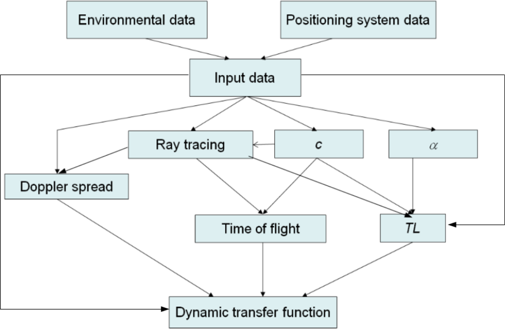
The block diagram of the model is shown in Figure 1. The inputs are environmental parameters, such as temperature, depth, salinity, bottom and water densities, wind speed or sound speed at bottom material; and the positioning system parameters, such as signal frequency, hydrophones’ depth, the aperture angle of the transducer or the position of the buoys. With all these data, the sound speed can be computed, as well as the absorption coefficient, α. Knowing the sound speed profile, the model performs a ray tracing in the considered environment, and computes the Doppler spread. With the information from the ray tracing and knowing the sound speed profile, the times of flight from the different arrivals are obtained, whereas the transmission loss (TL) is computed knowing the absorption coefficient, sound speed in water and in bottom material and using information from the ray tracing, such us the distance traveled by the rays, as well as some of the inputs of the model, like wind speed or signal frequency. The dynamic transfer function is then obtained using the internal Matlab function rayleighchan, which need as inputs the times of arrival for the different eigenrays as well as their transmission loss, the sampling frequency and the Doppler spread.
During the development of the model, its results were compared with the ones provided by the ray tracing code Bellhop [1], obtaining similar results. Additionally, in [24] a comparison between the model results and an experiment result found in the literature was conducted, showing a good performance.
2.2. Sound Speed
Sound speed in water c, can be theoretically obtained from the linear wave equation as Equation (1) [25]:
Sound speed is computed by Equation (2) for each layer of the water column, knowing the temperature profile and salinity, whereas pressure is obtained from the Leroy–Parthiot equation [27], which provides a depth to pressure conversion. A sound speed profile is then obtained and, considering it, the model can be applied both in shallow waters and deep waters. This sound speed profile is assumed to be constant in the present environment under study.
2.3. Transmission Loss
There are three main contributions to energy loss of an acoustic wave in water: geometrical spreading, absorption and rebounds at the surface and the bottom. This energy loss must be computed for each ray.
Geometrical spreading T Lgeo, is caused by the expansion of the acoustic wave through the medium. Depending on the geometry of the channel, there are two types of spreading: spherical and cylindrical. Geometrical spreading is computed by Equation (3), where r is the distance traveled by the ray and k is a constant which value is 10 for a cylindrical spreading (typical for shallow water environments) or 20 for a spherical spreading.
The model can compute the bottom loss T Lbot, by two means. One of them is the Rayleigh model [29], with which bottom loss is obtained by Equation (6):
As for the surface rebounds, one of the simplest equations to obtain the surface loss T Lsur, is the Beckmann–Spizzichino formula, in the form given by R. Coates in Equation (7) [30],
Adding together all the terms introduced before, the total transmission loss for each eigenray can be obtained by Equation (8), where the minus sign corrects the positive value of these magnitudes, and nbot, nsur are the total rebounds suffered by the ray at the bottom and the surface, respectively.
2.4. The Dynamic Effect of Swell
It has been previously stated that the surface is flat for computing the ray paths. However, the swell will cause a moving surface and a motion of the reflection point. This motion will cause a Doppler spread B in the surface-reflected signals, given by Equation (9) [31],
3. Relative Positioning System
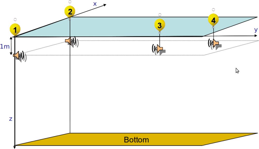
One of the main advantages of relative positioning systems is that only the distances between all the buoys are needed to obtain their positions. In this work, the relative positioning system consists of four buoys. Two of them are anchored at a fixed position: one of them is considered the origin of the coordinate system, so its position in the horizontal plane will always be (0, 0) m. The other fixed buoy helps define the axes of the Cartesian coordinate system by forming a line with the other buoy. Finally, the other two buoys can freely move through the sea surface.
At 1 m depth in each buoy there is a hydrophone, acting both as an emitter and receiver. The signal emitted by these hydrophones is supposed to be omnidirectional in the horizontal plane, but limited between ±20° in the vertical plane. Figure 2 shows the positioning system configuration.
For this simulated example, the buoys are supposed to be perfectly synchronized, e.g., by a RF link. As the errors in the system are in the order of a meter, as it is shown in Section 4, the system will be robust to synchronization errors up to approximately two hundred microseconds. These synchronization errors would cause a positioning error of the order of few decimeters. This tolerable synchronization error is greater than those found on the literature [32,33] for RF synchronization. An emission every three minutes is considered.
3.1. Coding Scheme
In order to obtain the times of flight more accurately, the acoustic signals are coded with CSS [34]. More specifically, preferred CSS are used, which provides best cross-correlation properties for this kind of sequences [35]. As the system consists of four buoys, four preferred CSS are needed. Every buoy emits a complementary set of four sequences, each of them of length 64. The sequences are interleaved and modulated in BPSK with a carrier frequency of 20 kHz, giving a total emission time of 12.8 ms.
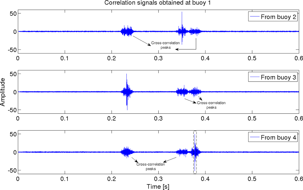
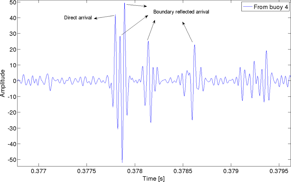
At each buoy, the received signal consists of the signals coming from the other three, which have suffered a fading obtained with the propagation model. Every buoy correlates this received signal with the CSS codes of the other three buoys, obtaining several correlation peaks, as can be seen in Figure 3, that shows an example for the signal received at buoy 1. Cross-correlation peaks have been marked in the figure, whereas Figure 4 shows a zoom of the autocorrelation peaks with the code from buoy 4. Several peaks can be detected, the first one coming from the direct arrival, and the other ones are boundary reflected paths. One of them has higher amplitude than the direct path, due to the particular phase interference. This is one of the sources of error in the measurement of the times of flight.
The measure of the time-of-flight (TOF) is done from the maximum amplitude peak from the correlation function. As the correlation peak is obtained when the entire coded signal has passed through the correlator, the TOF between two buoys (i, j) will be the difference between the time at which the maximum amplitude peak is detected, tij, and the duration of the emitted signal, tcode. Knowing these TOFs and the sound speed value computed at the hydrophone depth, c(z = 1 m), the distance between these buoys, dij, can be calculated by Equation (10). This formula does not provide errors for isovelocity profiles, like the one considered in this work, as it will be seen in Section 4.
3.2. MDS Positioning Algorithm
The buoys position are obtained with the MDS positioning algorithm [36]. To use the MDS technique, all the distances between the buoys are needed. This distances are computed by Equation (10) and collected into the matrix D, as seen in Equation (11),
To obtain the buoys positions, it is necessary to build another matrix H, called dot-product, whose elements Hij are obtained by Equation (12):
4. Results Using the Relative Positioning System
In this section, some simulated results using the relative positioning system are presented. A preliminary version of these results were presented at the OCEANS 2011 Conference [24], and the SAAEI 2011 Conference [37]. In this work, a statistical study of the performance of the system has been performed for different values of wind speed w, and SNR. Additionally, another set of simulations shows the tracking of two free-moving buoys at the surface for different simulation conditions.
The positioning system is simulated to be deployed in the coast of Comodoro Rivadavia, Argentina. The latitude of this city is −45.8647°, and it has a bottom depth of 6 m, few kilometers out to sea. This bottom is supposed to be sandy, with a density of 1, 941 kgm−3 and a sound speed of 1, 749 ms−1. A value of 1, 024 kgm−3 has been considered for the water density, as well as a salinity of 34.1‰ and a pH of 7. All these values are between the most common that one can encounter in the medium [38].
The value for the water temperature has been obtained by means of the Levitus Atlas [39]. The annual mean for the approximate latitude of Comodoro Rivadavia has been used, with a value of 8.1 °C. As the bottom depth is at 6 m, the system is deployed in a very shallow water environment, and thus, the temperature is assumed to be constant in all the water column, as well as the salinity, obtaining then a constant sound speed profile with the Chen–Millero equation.
4.1. Statistical Study of the System Behavior
Due to the statistical nature of the dynamic transfer function, a statistical study has been conducted. For each value of wind speed and SNR, a hundred simulations have been performed and the average error for each buoy has been obtained.
The positioning system consist of four buoys. The statistical study has been made considering only one position for all the buoys. The first buoy is fixed at (0, 0) m, whereas the second fixed buoy is placed at (0, 500) m. The position for the third buoy is (300, 125) m and for the fourth one, (450, 300) m.
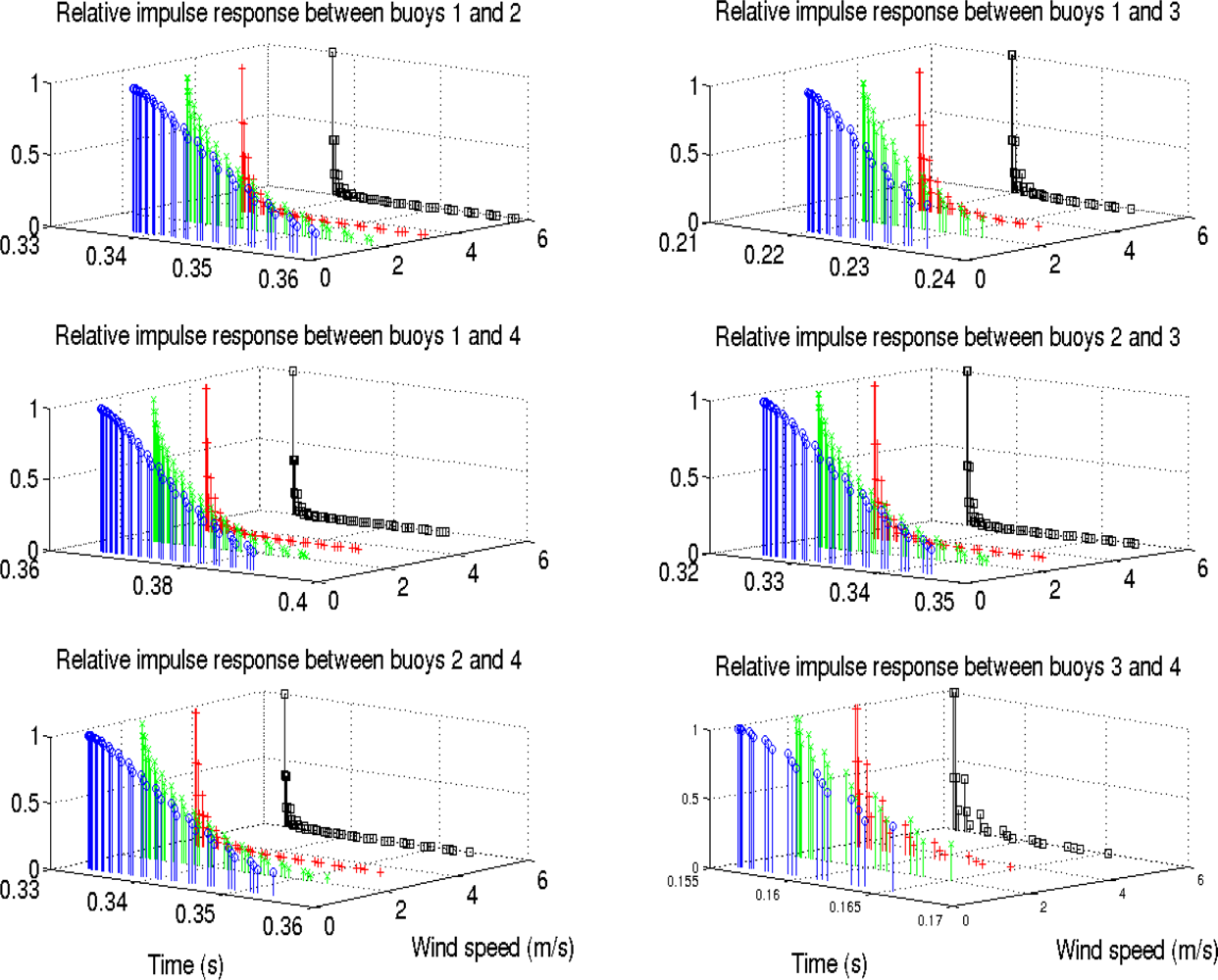
In this work, the SNR is defined as Eb/N0, where Eb is the energy per bit and N0 is the noise power spectral density, assuming an additive white Gaussian noise. The SNR values used were 12, 0 and −6 dB, obtaining three different situations with a strong signal in the first case, a noticeable noise in the second one and a very unfavorable situation in the third one. For the wind speed, four values were used: 0.5, 2, 3.5 and 6 ms−1, considering different situations ranging from almost no wind to a remarkable wind speed between them, where these values are easily found in Comodoro Rivadavia. The effect of the wind in the impulse response and the time spread can be seen in Figure 5, where the responses defined by each pair of buoys have been represented. Interference is expected between the signals of different buoys, as a severe multipath is present when there is almost no wind speed.
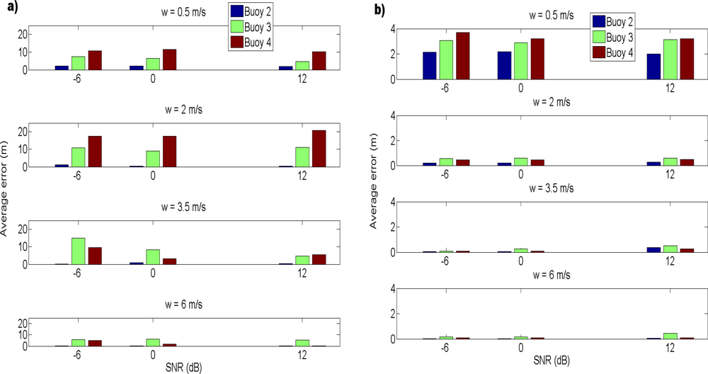
The results for the average error in each buoy, considering different values of SNR and wind speed are shown in Figure 6, where the values for the first buoy are not given, as this buoy is the origin and it is always considered fixed at (0, 0) m. In order to avoid the late arrivals due to multipath, as well as the detection of a maximum from another signal due to the near-far effect, a threshold of 10 m has been considered. Errors greater than 10 m has been identified as outliers and removed, after checking the histograms to verify that most of the errors were below 10 m. Figure 6(a) shows the results for all the simulations, whereas in Figure 6(b) the outliers have been taken out. Note the different scales used in the Y axes of Figure 6(a,b).
The first conclusion that can be drawn from these results is that outliers mask the behavior of the system. These outliers are due to the near-far effect, when a cross-correlation peak has a greater amplitude than an autocorrelation peak, causing greater errors in value, of tens or hundreds of meters, as the peak detected is from another buoy. As can be seen in Figure 6(a), the largest errors are obtained for buoys 3 and 4. Those buoys are close, and so this effect is more noticeable in them.
More interesting conclusions can be drawn by removing the outliers. First of all, the errors are now lower, as can be seen in Figure 6(b). Additionally, SNR does not seem to be crucial in the performance of the system for the parameters studied, obtaining practically the same errors for the three values of SNR used. However, wind speed seems to be determinant. For greater values of wind speed, the average error tends to decrease. Note that the greater the wind speed, the more surface loss per rebound, and the less multipath signals in the received signal, making easier the detection of the correct peak.
4.2. Tracking of the Movement Due to a Surface Current
In the statistical study, all the buoys were considered to be in a constant position. In this case, the two free-moving buoys will vary their positions due to a surface current. The objective is to track the buoys and obtain their positions at each time. Knowing the distance traveled and the time difference between emissions, the velocity and direction of the surface current could be determined.
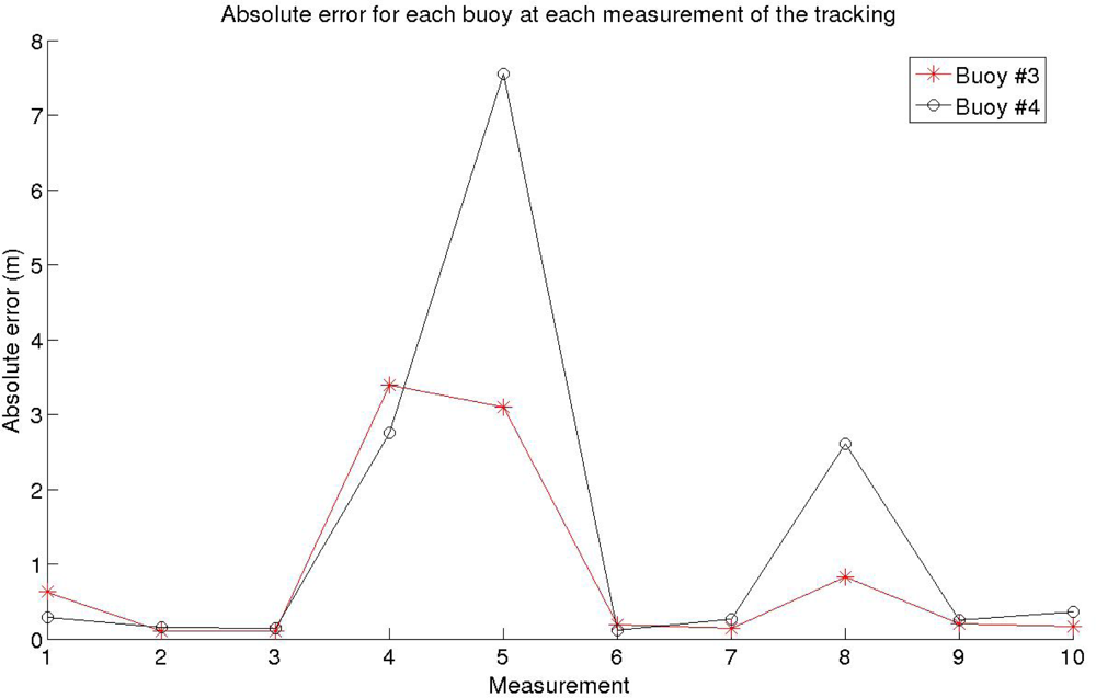
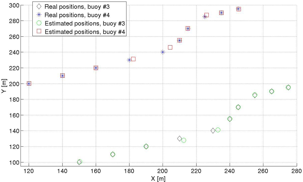
Both the SNR and the wind speed can vary from one position to the next one, as well as the value and direction of the surface current, to represent a realistic as possible situation. The fixed buoys were placed at (0, 0) m and (0, 300) m, and the moving buoys were placed initially at (150, 100) m and (120, 200) m. The results of the tracking can be seen at Figure 7, whereas Figure 8 shows the absolute error for each position and each buoy. The values for the SNR, wind speed w, and surface current for each measure are given in Table 2.
As shown in Figure 7, the relative positioning system is capable to correctly obtain the position of the buoys. At some specific positions, measurements 4 and 5 of the tracking, the error is between 2 and 6 meters greater, as can be clearly seen in Figure 8. This error is due to the low wind speed considered at that particular moment, as can be read in Table 2, causing that the received signal is highly affected by multipath. In the position number 8 there is also a low value of wind speed, which also provides an inaccuracy of 2 m in the worst case in the measurement of the buoys position, as shown in Figures 7 and 8. From measurement number 2 to number 3, there is a noticeable fall on the SNR (9 dB), but the system keeps working properly, showing that the SNR is not an important parameter for the values considered. Additionally, it can also be seen that this system would be capable to detect changes in the direction of the surface current, as well as its numerical value.
5. Summary and Conclusions
An underwater acoustic propagation model has been proposed in this work. This model takes into account a sound speed profile, so it can be used both in shallow waters and deep waters. Additionally, the equations that are used to compute the sound speed and transmission loss are valid in a wide range of input values, so it is not restricted to very specific environmental conditions. It also considers the dynamic effect of swell that worsens the properties of the surface-reflected signal and uses a dynamic transfer function.
Also, a relative positioning system has been presented. The performance of this system has been studied using the propagation model described before. For a particular position, the average error has been obtained for each buoy varying the SNR and the wind speed. Multipath caused by low wind speeds has been identified as the most damaging effect, and some outliers have been detected, due to the near-far effect, which disguise the behavior of the system.
As an early example of application, the relative positioning system has been used to track the position of the buoys, where two of them can freely move through the sea surface due to surface currents. The system is capable to track the positions in different times, so the value and direction of the surface current could be computed. Using the MDS algorithm, the error in these measurements is about 1 m usually, and 8 m in the worst case, unless outliers appear. No outliers appeared for the tracking of the moving buoys.
As future work, some improvements can be made into the model, like adding a bathymetry profile or a range-dependent option, so the performance of this system could be studied in more complex environments. The tracking of the surface buoys must be estimated continuously, so a fast algorithm with low computational complexity has been used (MDS). The outliers could be reduced by implementing refinement algorithms, which will increase the complexity of the system to the detriment of the time between measurements. Finally, it is important to remark that although the tracking of moving buoys in the surface is interesting, this is not the final application of this system. That would be the simultaneous positioning of buoys in the surface and submerged objects in the sea, where acoustic systems can work in more complex environments than other wireless techniques, whose use is severely limited underwater.
Acknowledgments
This work has been possible thanks to the support of the Spanish Ministry of Science and Innovation (TIN2009-14114-C04-01/04), the University of Alcalá (FPI fellowship) and the Regional Government of Extremadura through the European Regional Development Funds (FEDER - GR10097).
References
- Camargo, O. General description of the Bellhop ray tracing program. Available online: http://oalib.hlsresearch.com/Rays/GeneralDescription.pdf (accessed on 23 September 2011).
- Chitre, M. A High-frequency warm shallow water acoustic communications channel model and measurements. J. Acoust. Soc. Am 2007, 122, 2580–2586. [Google Scholar]
- Hovem, J.M.; Yan, S.; Bao, X.; Dong, H. Modeling Underwater Communication Links. Proceedings of the Second International Conference on Sensor Technologies and Applications, Cap Esterel, France, 25–31 August 2008; pp. 679–686.
- Buckingham, M.J. Ocean-acoustic propagation models. J. Acoust 1992, 223–287. [Google Scholar]
- Etter, P. Underwater Acoustic Modeling and Simulation, 3rd ed; Taylor and Francis: New York, NY, USA, 2003. [Google Scholar]
- Evans, R.B. A coupled mode solution for acoustic propagation in a waveguide with stepwise depth variations of a penetrable bottom. J. Acoust. Soc. Am 1983, 74, 188–195. [Google Scholar]
- Schmidt, H. Seismo-Acoustic Fast Field Algorithm for Range-Independent Environments. User’s Guide; SACLANT Undersea Research Centre: La Spezia, Italy, 1988. [Google Scholar]
- Goh, J.T.; Schmidt, H. A hybrid coupled wave-number integration approach to range-dependent seismoacoustic modeling. J. Acoust. Soc. Am 1996, 100, 1409–1420. [Google Scholar]
- Clark, J.A.; Sartori, M.A. Numerical Propagation of Spatially Distributed Acoustic Sources Using the Exterior Helmholtz Integral Equation. Proceedings of the IEEE Sixth SP Workshop on Statistical Signal and Array Processing, Victoria, BC, Canada, 7–9 October 1992; pp. 338–341.
- Wang, S. Finite-difference time-domain approach to underwater acoustic scattering problems. J. Acoust. Soc. Am 1996, 99, 1924–1931. [Google Scholar]
- Grilli, S.; Pedersen, T.; Stepanishen, P. A hybrid boundary element method for shallow water acoustic propagation over an irregular bottom. Eng. Anal. Bound. Elem 1998, 21, 131–145. [Google Scholar]
- Pereira, A.; Tadeu, A.; Godinho, L.; Santiago, J.A.F. 2.5D BEM modeling of underwater sound scattering in the presence of a slippage interface separating two flat layered regions. Wave Motion 2010, 47, 676–692. [Google Scholar]
- Collins, M.D. New and improved parabolic equation models. J. Acoust. Soc. Am 1998, 104, 1808A. [Google Scholar]
- Alcocer, A.; Oliveira, P.; Pascoal, A. Underwater Acoustic Positioning Systems Based on Buoys with GPS. Proceedings of the Eigth European Conference on Underwater Acoustics (ECUA 2006), Carvoeiro, Portugal, 12–15 June 2006.
- Kussat, N.H.; Chadwell, C.D.; Zimmerman, R. Absolute positioning of an autonomous underwater vehicle using GPS and acoustic measurements. IEEE J. Ocean. Eng 2005, 30, 153–164. [Google Scholar]
- Carroll, P.; Zhou, S.; Zhou, H.; Cui, J.H.; Willett, P. Underwater Localization Based on Multicarrier Waveforms. Proceedings of the IEEE OCEANS 2010 Conference, Seattle, WA, USA, 20–23 September 2010.
- Almeida, R.; Cruz, N.; Matos, A. Synchronized Intelligent Buoy Network for Underwataer Positioning. Proceedings of the IEEE OCEANS 2010 Conference, Seattle, WA, USA, 20–23 September 2010.
- Carevic, D. Localisation and Tracking of Underwataer Acoustic Source Using a Modified Particle Filter. Proceedings of the IEEE OCEANS 2010 Conference, Sydney, Australia, 24–27 May 2010.
- Peremans, H.; Audenaert, K.; Van Campenhout, J. A high resolution sensor based on tri-aural perception. IEEE Trans. Robot. Autom 1993, 9, 36–48. [Google Scholar]
- Jörg, K.-W.; Berg, M. Sophisticated mobile robot sonar sensing with Pseudo-Random codes. Robot. Auton. Syst 1998, 25, 241–251. [Google Scholar]
- Álvarez, F.J.; Ureña, J.; Mazo, M.; Hernández, A.; García, J.J.; De Marziani, C. High reliability outdoor sonar prototype based on efficient signal coding. IEEE Trans. Ultrason. Ferr 2006, 53, 1862–1871. [Google Scholar]
- De Marziani, C.; Ureña, J.; Hernández, A.; Mazo, M.; García, J.J.; Jiménez, A.; Pérez, M.C.; Álvarez, F.; Villadangos, J.M. Acoustic sensor network for relative positioning of nodes. Sensors 2009, 9, 8490–8507. [Google Scholar]
- Leighton, T.G. Fundamentals of Noise and Vibration; Fahy, F., Walker, J., Eds.; Spon Press: London, UK, 1998; pp. 373–443. [Google Scholar]
- Aparicio, J.; Álvarez, F.J.; Jiménez, A.; De Marziani, C.; Ureña, J.; Diego, C. Underwater Channel Modeling for a Relative Positioning System. Proceedings of the IEEE 2011 OCEANS Conference, Santander, Spain, 6–9 June 2011.
- Kinsler, L.E.; Frey, A.R.; Coppens, A.B.; Sanders, J.V. Fundamentals of Acoustics, 4th ed; John Wiley & Sons: New York, NY, USA, 2000. [Google Scholar]
- National Physical Laboratory. Technical guides: Speed of sound in sea-water. Available online: http://resource.npl.co.uk/acoustics/techguides/soundseawater/ (accessed on 14 July 2011).
- Leroy, C.C.; Parthiot, F. Depth-pressure relationships in the oceans and seas. J. Acoust. Soc. Am 1998, 103, 1346–1352. [Google Scholar]
- Domingo, M.C. Overview of channel models for underwater wireless communications networks. Phys. Commun 2008, 1, 163–182. [Google Scholar]
- Urick, R.J. Principles of Underwater Sound, 3rd ed; Peninsula Publishing: Los Altos Hills, CA, USA, 1983. [Google Scholar]
- Coates, R. An empirical formula for computing the Beckman-Spizzichino surface reflection loss coefficient. IEEE Trans. Ultrason. Ferr 1988, 35, 522–523. [Google Scholar]
- Stojanovic, M. Wiley Encyclopedia of Telecommunications; Proakis, J.G., Ed.; John Wiley & Sons: New York, NY, USA, 2003; Volume 1, pp. 36–47. [Google Scholar]
- Cox, D.; Jovanov, E.; Milenkovic, A. Time Synchronization for ZigBee Networks. Proceedings of the Thirty-Seventh Southeastern Symposium on System Theory, Tuskegee, AL, USA, 20–22 March 2005; pp. 135–138.
- Ferrari, P.; Flammini, A.; Marioli, D.; Sisinni, E.; Taroni, A. Non Invasive Time Synchronization for ZigBee Wireless Sensor Networks. Proceedings of the International IEEE Symposium on Precision Clock Synchronization for Measurement, Control and Communication, Ann Arbor, MI, USA, 22–26 September 2008; pp. 121–126.
- Tseng, C.C.; Liu, C.L. Complementary sets of sequences. IEEE Trans. Inform. Theory 1972, 18, 644–652. [Google Scholar]
- De Marziani, C.; Ureña, J.; Hernández, A.; Álvarez, F.J.; Mazo, M.; García, J.J.; Jiménez, A.; Villadangos, J.M.; Pérez, M.C.; Ochoa, A. Inter-Symbol Interference Reduction on Macro-Sequences Generated from Complementary Set of Sequences. Proceedings of the 32nd Annual Conference of the IEEE Industrial Electronics Society (IECON 06), Paris, France, 7–10 November 2006; pp. 3367–3372.
- Torgerson, W.S. Multidimensional Scaling: I. Theory and Method. Psychometrika 1952, 17, 401–419. [Google Scholar]
- Aparicio, J.; Jiménez, A.; Álvarez, F.J.; De Marziani, D.; Sanz, R.; Diego, C. Modelado de canal subacuático dinámico para un sistema de posicionamiento relativo ultrasónico (in Spanish in the original). Proceedings of the XVIII Edition of the Annual Seminar on Automatics, Industrial Electronics and Instrumentation (SAAEI 2011), Badajoz, Spain, 5–8 July 2011; pp. 879–884.
- Jensen, F.B.; Kuperman, W.A.; Porter, M.B.; Schmidt, H. Computational Ocean Acoustics; Springer-Verlag: New York, NY, USA, 2000. [Google Scholar]
- National Oceanographic Data Center. Climatologial Atlas of the World Ocean. Available online: ftp://ftp.nodc.noaa.gov/pub/data.nodc/woa/PUBLICATIONS/levitus_atlas_1982.pdf (accessed on 15 July 2011).


| Parameter | Value | Parameter | Value | Parameter | Value |
|---|---|---|---|---|---|
| C00 | 1402.388 | C01 | 5.03830 | C02 | −5.81090E-2 |
| C03 | 3.3432E-4 | C04 | −1.47797E-6 | C05 | 3.1419E-9 |
| C10 | 0.153563 | C11 | 6.8999E-4 | C12 | −8.1829E-6 |
| C13 | 1.3632E-7 | C14 | −6.1260E-10 | C20 | 3.1260E-5 |
| C21 | −1.7111E-6 | C22 | 2.5986E-8 | C23 | −2.5353E-10 |
| C24 | 1.0415E-12 | C30 | −9.7729E-9 | C31 | 3.8513E-10 |
| C32 | −2.3654E-12 | A00 | 1.389 | A01 | −1.262E-2 |
| A02 | 7.166E-5 | A03 | 2.008E-6 | A04 | −3.21E-8 |
| A10 | 9.4742E-5 | A11 | −1.2583E-5 | A12 | −6.4928E-8 |
| A13 | 1.0515E-8 | A14 | −2.0142E-10 | A20 | −3.9064E-7 |
| A21 | 9.1061E-9 | A22 | −1.6009E-10 | A23 | 7.994E-12 |
| A30 | 1.100E-10 | A31 | 6.651E-12 | A32 | −3.391E-13 |
| B00 | −1.922E-2 | B01 | −4.42E-5 | B10 | 7.3637E-5 |
| B11 | 1.7950E-7 | D00 | 1.727E-3 | D10 | −7.9836E-6 |
| Measurement | SNR (dB) | w (ms−1) | Surface current (ms−1) |
|---|---|---|---|
| 1 | 6 | 2.5 | (0.11,0.06) |
| 2 | 6 | 2.5 | (0.11,0.06) |
| 3 | −3 | 2.5 | (0.11,0.06) |
| 4 | 6 | 0.6 | (0.11,0.06) |
| 5 | −6 | 0.6 | (0.06,0.08) |
| 6 | 3 | 4 | (0.03,0.08) |
| 7 | 3 | 4 | (0.06,0.08) |
| 8 | 3 | 1 | (0.06,0.03) |
| 9 | 6 | 2 | (0.06,0.03) |
| 10 | 6 | 2 | (0,0) |
© 2011 by the authors; licensee MDPI, Basel, Switzerland. This article is an open access article distributed under the terms and conditions of the Creative Commons Attribution license (http://creativecommons.org/licenses/by/3.0/).
Share and Cite
Aparicio, J.; Jiménez, A.; Álvarez, F.J.; Ureña, J.; Marziani, C.D.; Diego, C. Modeling the Behavior of an Underwater Acoustic Relative Positioning System Based on Complementary Set of Sequences. Sensors 2011, 11, 11188-11205. https://doi.org/10.3390/s111211188
Aparicio J, Jiménez A, Álvarez FJ, Ureña J, Marziani CD, Diego C. Modeling the Behavior of an Underwater Acoustic Relative Positioning System Based on Complementary Set of Sequences. Sensors. 2011; 11(12):11188-11205. https://doi.org/10.3390/s111211188
Chicago/Turabian StyleAparicio, Joaquín, Ana Jiménez, Fernando J. Álvarez, Jesús Ureña, Carlos De Marziani, and Cristina Diego. 2011. "Modeling the Behavior of an Underwater Acoustic Relative Positioning System Based on Complementary Set of Sequences" Sensors 11, no. 12: 11188-11205. https://doi.org/10.3390/s111211188