High Dynamic Velocity Range Particle Image Velocimetry Using Multiple Pulse Separation Imaging


Abstract
: The dynamic velocity range of particle image velocimetry (PIV) is determined by the maximum and minimum resolvable particle displacement. Various techniques have extended the dynamic range, however flows with a wide velocity range (e.g., impinging jets) still challenge PIV algorithms. A new technique is presented to increase the dynamic velocity range by over an order of magnitude. The multiple pulse separation (MPS) technique (i) records series of double-frame exposures with different pulse separations, (ii) processes the fields using conventional multi-grid algorithms, and (iii) yields a composite velocity field with a locally optimized pulse separation. A robust criterion determines the local optimum pulse separation, accounting for correlation strength and measurement uncertainty. Validation experiments are performed in an impinging jet flow, using laser-Doppler velocimetry as reference measurement. The precision of mean flow and turbulence quantities is significantly improved compared to conventional PIV, due to the increase in dynamic range. In a wide range of applications, MPS PIV is a robust approach to increase the dynamic velocity range without restricting the vector evaluation methods.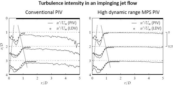
1. Introduction
In particle image velocimetry (PIV), a flow is seeded with tracer particles and illuminated by a pulsed light sheet, yielding a series of image pairs with a pulse separation τ. After subdividing the images into interrogation windows, spatial cross-correlation yields the window-averaged particle displacement. The general theory and design rules for PIV have been established by e.g., Keane and Adrian [1,2]. Since the early 1990s, progressive improvements have been made to velocity evaluation methods. Some key contributions are reviewed below in terms of their influence on the dynamic velocity range DRV, corresponding to the ratio of maximum to minimum resolvable velocity:
1.1. Single-Pass Correlation
To avoid loss of correlation due to excessive in-plane displacement, Keane and Adrian [1] state that the displacement s should be smaller than one quarter of the interrogation window size dI, or . This yields a maximum value for the pulse separation τ for a given velocity magnitude U and pixel scaling M [m/px]. Smaller τ values result in a slightly stronger correlation; however the displacement should remain greater than the minimum resolvable displacement. Incorporating this rule, the dynamic velocity range for single-pass correlation is
Raffel et al. [3] and Westerweel [4] review the dependence of the total displacement error (and thus σs) on a number of parameters for single-pass correlation (e.g., particle displacement, number density and diameter, interrogation window size, image background noise, velocity gradients).
1.2. Multi-Pass Correlation
Westerweel et al. [5] describe a multi-pass correlation approach by shifting windows over discrete pixel amounts, based on the local displacement obtained in the previous pass. Simulation results show a threefold reduction in displacement uncertainty Δsrms. Validation results of grid-generated turbulence in a water channel show a typical displacement uncertainty of 0.04 px, compared to 0.095 px without window shifting [5]. The technique has since been improved to continuous shifting, applying image interpolation techniques [6].
Scarano and Riethmuller [7] describe an iterative window deformation method with progressive grid refinement. Monte Carlo simulations of noiseless artificial images yield uncertainty values of about 10−3 px [8]. Multi-grid techniques partly decouple the maximum displacement and final window size, since the 1/4 window rule [1] only applies to the first (coarse) grid. For a progressive refinement from an initial window kgdI to final window dI (kg > 1), Equation (2) can be rewritten as:
For the same final window (dI), DRV increases by the grid refinement ratio (typically 2 ≤ kg ≤ 4). A further increase is due to a reduction of σs. Westerweel [5] and Scarano and Riethmuller [6] report an uncertainty reduction σs(s)/σs(m) ≅ 3 for discrete window shifting and σs(s)/σs(m) ≅ 10 for subpixel window shifting and deformation, respectively. However, these values are obtained for noiseless artificial images and the uncertainty increases for more realistic conditions, e.g., non-zero gradients [9].
In the remainder of the paper, ‘conventional’ PIV refers to the current state of art multi-grid cross-correlation using subpixel window shifting and deformation.
1.3. Multi-Frame (MF) Correlation: Locally Increasing Pulse Separation
Increasing the pulse separation to enhance the dynamic range is generally not preferred. However some studies present satisfactory results when the increase is applied locally [10–12]. These techniques use single-frame imaging, and are proposed as alternatives to multi-grid methods.
Fincham and Delerce [10] suggest a multi-frame (MF) approach based on a series of single-frame recordings, where an initial correlation of two frames (separated by inter-frame time δt) is used as a displacement estimate for the deformation and correlation of frames separated by 2δt or 3δt. This aim is to increase the average pixel displacement, thus improving the dynamic velocity range.
Hain and Kähler [11] also propose an iterative MF technique to compensate for the loss in dynamic range of CMOS sensors used in high speed PIV systems, compared to CCD sensors. On a single-frame sequence {...t − 2δt, t − δt, t, t + δt, t + 2δt...}, an initial correlation is performed on frames t − δt and t + δt. The correlation is repeated between frames t − kτδt and t + kτδt, where the multiplier kτ is estimated based on the quarter window rule assumption and the local displacement s, as . In selecting the optimal kτ, Hain and Kähler [11] indicate that a simple threshold for the correlation peak ratio Q (i.e., ratio of highest to second highest correlation peak [1]) is not sufficient for optimality. The authors assume a minimum resolvable displacement of 0.1 px.
Multi-frame PIV is most suitable for low speed flows. Hain and Kähler [11] validate their technique with direct numerical simulations of a laminar separation bubble (Umax = 0.15 m/s) and experimental velocity data around an airfoil in water (Umax = 0.1 m/s). Pereira et al. [12] propose a similar MF technique and compare it to multi-grid PIV, for test cases including artificial particle images (Umax = 1 px/s and δt = 1 s) and a laminar water flow (Umax = 0.05 m/s). In these cases with a wide velocity range, MF PIV has achieved good results compared to conventional PIV. However, since MF PIV is proposed as an alternative to multi-grid algorithms, it cannot benefit from advances in this field.
1.4. Objectives
This paper proposes a new multiple pulse separation (MPS) technique to increase the dynamic velocity range of PIV. The technique is based on double-frame imaging, thus avoiding the low speed restriction and excessive pulse separations of MF PIV [10–12]. It does not exclude the use of multi-grid algorithms. A robust criterion for pulse separation optimality is established and validated.
2. Proposed Methodology: Multiple Pulse Separation (MPS) PIV
2.1. Basics of MPS PIV
Consider a flow field with a wide range in velocity magnitude (e.g., a jet or wake flow), where Umax and Umin represent two characteristic velocity scales in the high and low velocity regions, respectively. As the ratio Umax/Umin approaches the dynamic velocity range of the measurement technique (DRV), the vector quality in the low velocity region deteriorates. For this reason multi-frame correlation was first proposed [10–12]. By selectively applying a higher pulse separation kττ only in the low velocity region, the minimum measurable velocity reduces (σV ∝ σs/(kττ)) and the dynamic velocity range increases:
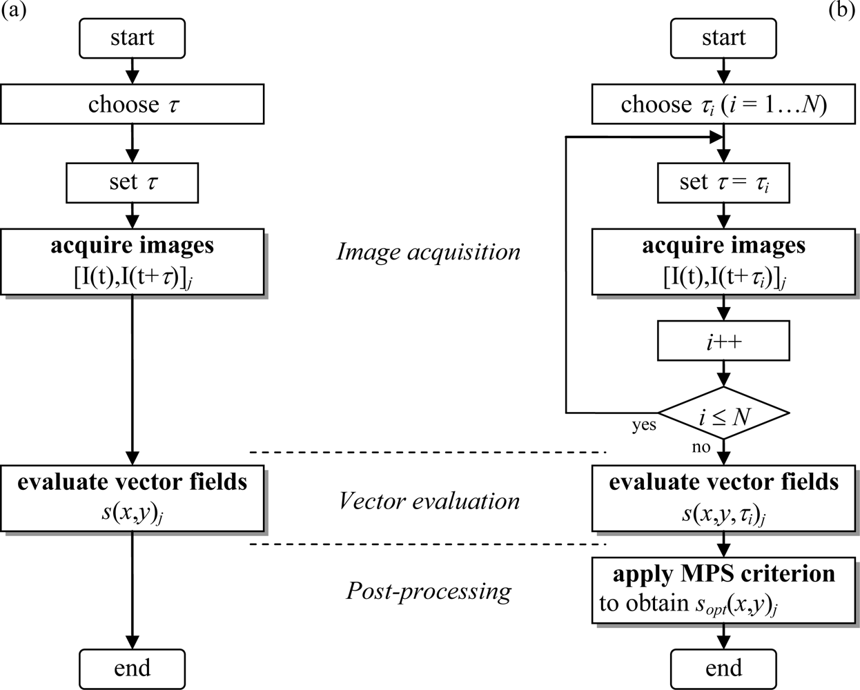
Contrary to the multi-frame approach [10–12], multi pulse separation (MPS) PIV acquires double-frame images {...,[t, t + kτ,1τ], [t + δt, t + δt + kτ,2τ],...} with N different pulse separation values kτ,iτ (i = 1…N) at a frame rate 1/δt, where the N multipliers kτ,1, kτ,2, … kτ,N represent monotonically increasing values (e.g., 1, 4, 16). Figure 1(a) depicts the conventional double-frame (single exposure) PIV approach with a single fixed pulse separation τ. The subscript j is the index in the sequence of acquired image pairs, and the subsequently evaluated displacement fields s⃗ (x,y)j the arrow notation is often omitted hereafter). Figure 1(b) depicts the MPS PIV approach: (i) a sequence of double-frame images [I(t), I(t+τi)]j is acquired, while the pulse separation loops through N chosen values (τi = kτ,iτ). Next (ii) the vector fields for all pulse separation values are evaluated using conventional multi-grid algorithms. Finally (iii) the pulse separation optimality criterion (described below) is applied in a post-processing step, resulting in the final displacement fields s⃗opt(x,y)j.
2.2. Optimality Criterion for Pulse Separation
The peak ratio Q is a measure of the correlation strength of a displacement vector [1]. To assess the local precision, the displacement magnitude |s| is compared to the minimum resolvable displacement σs. As a precision measure, 1 − σs/|s| varies between unity for |s| σs, over zero for |s| = σs to -∞ as |s| → 0. The weighted peak ratio Q’ is defined as a measure of local vector quality, combining correlation strength and precision:
The pulse separation optimality criterion is based on the local maximum of Q’. In each point (x, y), the local maximum of Q’ = Q’(x,y,τi) = Q(x,y,τi) (1 − σs/‖s⃗(x,y,τi)‖) the local optimum pulse separation. The approach assumes that the value of σs does not vary significantly within the field of view, which is true for typical laboratory conditions with background image noise and velocity gradients. Although advanced multi-grid algorithms can attain errors below 0.001 px in noiseless conditions [6,8], a value for σs in more realistic conditions is about 0.1 px. In the optimality criterion, values of σs between 0.05 px and 0.2 px yield the best results. This order of magnitude seems appropriate for multi-grid algorithms in realistic conditions, based on validation results in the review of Stanislas et al. [13].
A selector operator is defined based on the maximum Q’ value:
The optimal pulse separation, displacement and velocity fields are determined as
Based on Equation (7), each vector is taken from a single measurement according to the local maximum Q’ value. An alternative definition is based on a linear combination, weighted according to the value of Q’. A relaxed maximum selector is therefore defined as
Using Equation (8) the optimal displacement, velocity and pulse separation are
The optimality criterion based on the relaxed maximum (Equation (9)) yields smoother results since data obtained at different pulse separations are combined, weighted by the local Q’ value. The exponent p determines the relative contribution of data obtained at sub-optimal pulse separations. In practice p = 5 yields good results, while the difference between Equations (7) and (9) is negligible for p > 20.
In choosing the pulse separation multipliers kτ,i (i = 1…N), the smallest value τ (kτ,1 = 1) should limit the correlation loss in the high velocity region, based on e.g., the 1/4 window rule [1] or similar considerations. The maximum kτ,N can be chosen analogously for the low velocity region, e.g., as. kτ,N ≅ Umax/Umin Regarding the total number of values, N = 2 or 3 typically yields good results while limiting the additional acquisition and processing time.
Compared to conventional PIV, the maximum increase in dynamic velocity range is (see Equation (4)), where kτ,max < kτ,N since the optimality criterion does not necessarily select the largest applied pulse separation. From Equation (4), the actual dynamic velocity range for MPS PIV is given by
2.3. Analogy to High Dynamic Range (HDR) Photography
Mann and Picard [14] introduced a technique to combine photographic images with different exposure times, to extend the dynamic intensity range beyond the restrictions of a digital sensor. A composite high dynamic range (HDR) image is generated as the weighted sum of all images. Weighting or ‘certainty’ functions are determined to favour mid-range intensity values, corresponding to the maximal sensor sensitivity and avoiding clipping near the edges of the range. Reinhard et al. [15] and Battiato et al. [16] discuss several weighting approaches to match the nonlinear response curve of an optical sensor array.
The MPS PIV technique proposed in this paper shows some analogies to HDR imaging. In both cases, a high dynamic range composite field is generated from a set of low dynamic range fields with different ‘exposure times’. Similarities persist in the optimality criterion used to construct the composite field. In HDR imaging, continuous weighting functions are used to provide a gradual transition between dark (underexposed) and bright (overexposed) regions. Thus each pixel contains information from all images in the set. MPS PIV also uses continuous weighting functions based on the local weighted peak ratio Q’, given by the relaxed maximum criterion (Equations (8) and (9)). However, a high exponent (p ≅ 5) is applied in Equation (8) to limit the contribution of data obtained at sub-optimal pulse separation values. In the extreme case where p → ∞, Equation (8) tends to Equation (6) and becomes a strict maximum selector, where each vector is selected from a single pulse separation acquisition.
The contribution of data from sub-optimal pulse separations should be limited in MPS PIV due to the strongly nonlinear nature of the correlation peak detection in PIV. Spurious vectors for excessive pulse separation values must not be allowed to propagate into the composite velocity field. As for any other technique, MPS PIV should be applied with good judgment.
2.4. Applicability and Limitations
Similar to conventional PIV, MPS PIV is applicable to stationary or non-stationary flows. MPS PIV correlates double-frame images separated by τi, whereas MF PIV correlates single-frame images separated by multiples of δt. Determined by the system repetition rate fF, the minimal δt far exceeds the minimum pulse separation for double-pulsed systems (τ 1/fF,max ≤ δt). This is a significant distinction between MPS and MF PIV. Excessive particle displacement limits MF PIV to low speed flows. Hain and Kähler [11] and Pereira et al. [12] report maximum velocities below 0.1 m/s in practical applications. Using double-frame imaging, MPS PIV is applicable to low and high speed flows in the same way as conventional PIV.
For temporal or spectral analyses, the common limitation for MPS and MF techniques is that a single recording duration Nδt (or N/fF) should be smaller than the flow time scale, where N is the number of pulse separations. The same restriction applies to conventional PIV, albeit for N = 1.
For amplitude domain analysis, no restrictions apply for single-point statistics (e.g., mean, variances and Reynolds stresses, higher order moments, probability density functions). For two-point statistics (e.g., spatial correlation) only point pairs acquired at the same measurement time should be considered.
MPS PIV is not an alternative but an addition to multi-grid techniques, without restricting the use of advanced methods such as window shifting and deformation. For the validation results (Section 3), the technique is implemented as a set of macro functions in LaVision Davis 7.2.2, using its multi-grid algorithms with deformation for vector evaluation.
3. Experimental Validation
The proposed methodology is validated based on experimental PIV data, obtained in an axisymmetric impinging jet. Two references are used for this validation: (i) Firstly, the precision of the mean and rms velocity is compared against laser-Doppler velocimetry (LDV). Secondly, the accuracy of the radial mass flux is verified against the mass conservation law.
3.1. Description of the Test Case
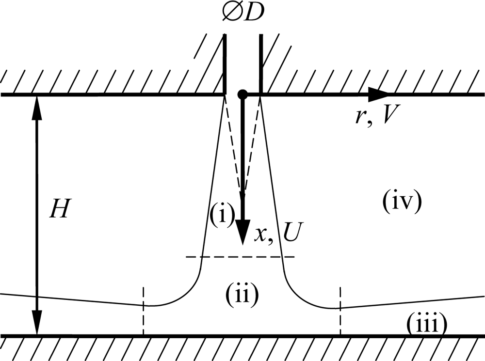
A single round stationary jet of air impinges perpendicularly onto a flat surface (Figure 2). The orifice diameter D = 5 mm and the orifice-to-surface distance H = 4D. The axial and radial coordinates x and r are aligned along the jet axis and perpendicular to it, respectively. The jet issues from a straight-edged orifice of length 2D, connected to a settling chamber. The velocity distribution in the orifice is axisymmetric yet not radially uniform. This is not important for the test case, and no effort was made to prevent flow separation at the upstream orifice edge. The flow rate is measured and maintained constant using a digital mass flow controller (MKS 1579A, 300 standard litres/min, repeatability ±0.2%). All experiments are performed at a fixed Reynolds number of Re = 8,000, based on D and the mean velocity in the jet orifice (Um = 24 m/s). Fitzgerald and Garimella [17] present velocity distributions measured using LDV in a similar geometry for Re = 8,500.
Figure 2 identifies four distinct regions in the flow field: (i) the free jet with a decaying potential core in the centre and surrounding shear layer, (ii) the stagnation region, (iii) the wall jet and (iv) the entrainment region. Each of these features a significantly different characteristic velocity magnitude, making this an interesting test case for the proposed methodology.
The PIV system comprises a New Wave Solo-II Nd:YAG twin cavity laser (30 mJ, 15 Hz) and a LaVision FlowMaster 3S (PCO SensiCam) thermo-electrically cooled CCD camera (1,280 × 1,024 px2, 12 bit) with 28 mm lens. The image magnification is 1:3.4 (M = 45 μm/px). A glycol-water aerosol is used for seeding, with particle diameters between 0.2 and 0.3 μm. The particle image diameter is adjusted to dp ≅ 2 px by defocusing slightly. Customized optics generate a 0.3 mm thick light sheet. The CCD camera is mounted perpendicular to the light sheet. The velocity fields are processed with LaVision’s DaVis 7.2.2 software, using multi-grid cross-correlation with continuous window shifting and deformation, with a window size decreasing from 64 × 64 px2 to 32 × 32 px2 and a 75% overlap. The validation is based only on amplitude domain statistics (mean flow and turbulence intensities). As such, a low speed PIV system can be used in this stationary flow configuration.
The LDV system comprises a 500 mW Ar+ laser and a dual beam Dantec optics with 488 nm (blue) and 514 nm (green) wavelengths to measure axial (along x) and radial (along r) velocity components, respectively. The optical head applies Bragg cell frequency shifting to both components. The system is operated in backscattering mode to facilitate translation and near-wall measurements. The measurement volumes are about 0.12 mm in diameter and 1.6 mm long, with the long axis aligned in the out-of-plane (z) direction. The same aerosol seeding is used. The velocity data are evaluated using a Dantec BSA F50 burst spectrum analyser. Velocity weighting and statistics are performed using Matlab, applying inverse velocity magnitude weighting to reduce high velocity bias errors.
3.2. Comparison of Conventional versus MPS PIV
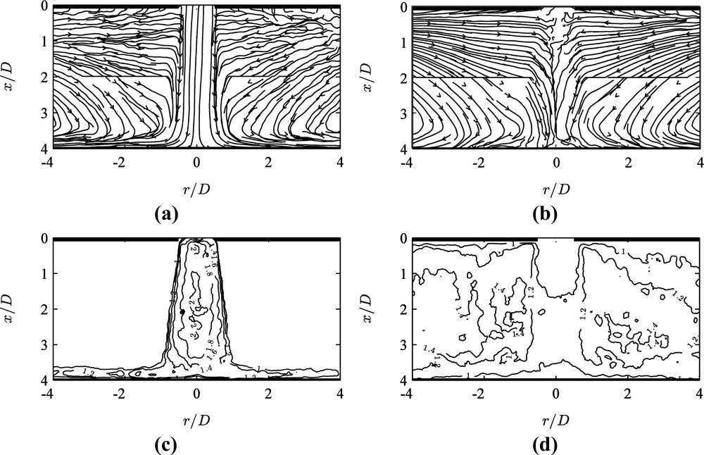
Figure 3(a) shows a time-averaged streamline plot for the jet flow obtained using conventional PIV. The term ‘conventional’ here denotes the best possible selection of the pulse separation τ = τmin which maximizes vector quality throughout the field of view, and the same above described algorithm. The quarter window rule in this case suggests , however a further reduction was needed due to strong gradients in the shear layer. To limit correlation loss due to gradients, Westerweel [9] derived a pulse separation threshold as (for single pass correlation). For a shear layer gradient ∂U/∂x ≅ Umax/(D/2) = 9,600 s−1, the threshold yields τ < 4.3 μs. In practice, a maximum value of τ (= τmin) = 5 μs was found to ensure good vectors in the shear layer, resulting in a displacement of about 3 px in the jet core, and a gradient of ds/dr(dI/dp) ≅ 0.75 px/px in the shear layer. The strong gradient is the limiting factor here, yet the value of 0.75 px/px is comparable to that achieved by other authors in strong shear flows using multi-grid correlation [8]. Attempts to further increase τ (e.g., by decreasing the initial window) resulted in invalid vectors in the shear layer region.
Figure 3(b) shows the corresponding results for a 10 times larger pulse separation τ = 10τmin, yet otherwise identical acquisition and processing parameters. In the high velocity jet core region, the streamlines break down due to the absence of valid vectors, whereas the low velocity region shows smoother streamlines for τ = 10τmin than the ones for τ = τmin in Figure 3(a).
The MPS technique proposes the weighted peak ratio Q’ = Q(1 – σs/|s|) as a measure of local pulse separation optimality. Distributions of Q’ are plotted in Figure 3(c,d). For both pulse separation values, the region of best vector quality corresponds to high values of Q’. These occur in the jet core and wall jet region for small pulse separation τ = τmin (Figure 3(a,c)) and in the entrainment region for the larger pulse separation τ = 10τmin (Figure 3(b,d)).
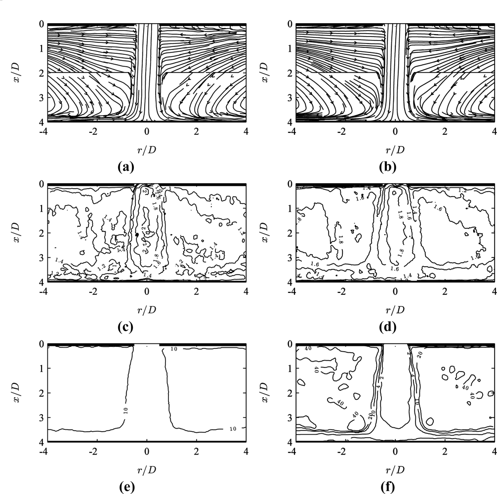
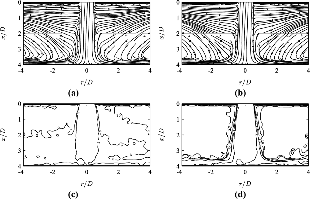
Figure 4(a,c,e) shows the corresponding MPS PIV results after applying the optimality criterion (σs = 0.2 px and p = 5 in Equation (8)) to the data obtained at two pulse separation values τ/τmin = {1, 10}. Figure 4(b,d,f) shows MPS results for data acquired at seven values τ/τmin = {1, 2, 4, 10, 20, 40, 100}.
Figure 4(e,f) shows the distribution of the optimal pulse separation τopt(x,y)/τmin. The smallest values τ ≅ τmin are used in the jet core region, and larger values τ ≅ 10τmin in the entrainment region. When applying a larger number of pulse separations, Figure 4(f) shows that intermediate values 2 < τ/τmin < 4 are used for the stagnation and wall jet regions, and high values 10 < τ/τmin < 40 in the lowest velocity regions.
3.2.1. Effect of Optimality Criterion Parameters
Figure 5 shows the influence of the optimality criterion parameters (σs and p in Equation (8)) on the MPS PIV results. With a lower value of σs (= 0.02 px), Figure 5(a,c) shows the criterion giving preference to high correlation strength rather than large pulse separation values, although a larger pulse separation (τ ≅ 10τmin) is still applied in the outer entrainment region. As σs → 0 px, Q’ → Q and thus the criterion selects the pulse separation corresponding to the maximum correlation peak ratio.
Figure 5(b,d) shows the effect of the strict maximum selector (Equation (6)), corresponding to p → +∞ in Equation (8). In this case, each vector is selected from a single pulse separation acquisition. The resulting distribution of the optimal pulse separation in Figure 5(d) shows discrete steps in pulse separation values applied throughout the flow field.
Comparing Figures 4 and 5, the effect of the criterion parameters on the streamline plot is not very significant. In that sense, the criterion is quite robust against parameter changes. However closer inspection of the results does allow optimisation of the criterion parameters σs and p.
3.2.2. Actual Increase of Dynamic Velocity Range
Based on Equation (10) and the results shown in Figure 4(f), the actual increase in dynamic velocity range can be determined. The ratio of local maximum to minimum pulse separation kτ = max(τopt)/τmin ≅ 40. Therefore MPS has increased the dynamic velocity range by kτ ≅ 40 = 101.6 times compared to the conventional multi-grid PIV approach. Determining the exact dynamic range based on Equation (10) is not straightforward. Assuming σs(m) ≅ 0.1 px and kgdI = 64 px, DRV(m) ≅ 160:1 (= 102.2). With this assumption, the dynamic range of MPS PIV is DRV(mps) ≅ 6,400:1 (= 103.8).
Although data was available at a higher pulse separation (τ = 100τmin), the optimality criterion has not used this, since the weighted peak ratio for τ = 100τmin is lower than for τ = 40τmin even in the low velocity region. This demonstrates that the technique does not necessarily select the largest pulse separation over the optimal value.
A dynamic velocity range of four orders of magnitude (104:1) has already been quoted in the literature for multi-grid algorithms using a single pulse separation [6,8]. However, those values correspond to simulation results for noiseless artificial particle images, whereas this value of DRV(mps) ≅ 6,400:1 (or 3.8 orders of magnitude) is obtained in laboratory conditions for a real jet flow.
3.3. Validation against Independent References
3.3.1. Validation against Laser-Doppler Velocimetry
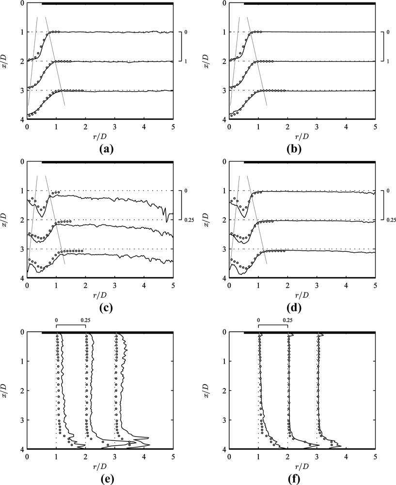
Figure 6 presents profiles of mean flow and turbulence intensity obtained using conventional (left) and MPS PIV (right) in the impinging jet. These quantities are defined as and , where Uj are the instantaneous velocity fields (j = 1…n) with analogous expressions for V and v’. All MPS PIV results hereafter correspond to the data in Figure 4(b) obtained at seven pulse separation values 1 ≤ τ/τmin ≤ 100, with σs = 0.2 px and p = 5 in Equation (8). The circular markers represent measurements using the laser-Doppler velocimeter (LDV) described in Section 3.1. The extent of the jet core and outer shear layer is indicated by thin lines in Figure 6 (a–d). All velocities are normalised to the mean orifice velocity Um (= 24 m/s for Re = 8000).
In Figure 6(a,b), the time-averaged velocity results of conventional PIV, MPS PIV and LDV show a good agreement in the central region (r/D < 2) to within 5% deviation. The conventional PIV results exhibit some residual noise from averaging bad vectors in the low velocity region (r/D > 2), whereas the MPS PIV profiles are much smoother.
The difference is even clearer for the rms velocity fluctuations u’ and v’ (Figure 6(c–f)). The conventional PIV results only agree with LDV in the central region (r/D < 0.75) to within 5% (Figure 6(c)). However in the outer shear layer (r/D ≅ 1), conventional PIV overpredicts the turbulence intensity by about 2.5 times. In the entrainment region, conventional PIV falsely predicts a turbulence level of about 7.5% for 1.5 < r/D < 4, increasing up to 20% for r/D > 4. This behaviour has no physical ground, since LDV results by Fitzgerald and Garimella [17] confirm a turbulence intensity below 2% for r/D > 1.5 (for Re = 8500). This is verified in the MPS PIV turbulence intensity values of about 1.5% for 1.5 < r/D < 4 (Figure 6(d)).
Radial turbulence intensity profiles intersecting the wall jet region (Figure 6(e)) show an overprediction of about 7.5% for conventional PIV. Figure 6(f) shows a much better agreement in the wall jet region for MPS PIV, with an average deviation below 2%. The magnitude and location of the turbulence peak in the wall jet agrees well for MPS PIV and LDV results.
This validation against LDV shows that conventional PIV overestimates the turbulence intensity because the displacement magnitude reduces to the minimum resolvable level σs, resulting in a poor velocity resolution. MPS PIV yields more precise results due to the increase in dynamic velocity range and reduction in minimum resolvable velocity (σV ∝ min(σs/τopt)).
3.3.2. Validation against Conservation of Mass
The increase in accuracy when applying MPS PIV can be quantified by verifying the conservation of mass in the flow field. For an axisymmetric impinging jet, the net mass flow rate ṁ(r) exiting a cylindrical control volume of radius r (see Figure 2) is given by:
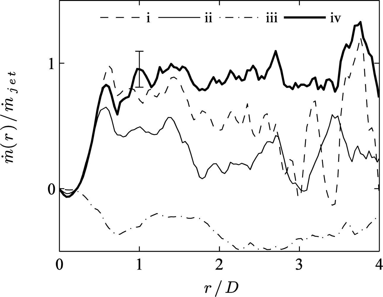
Figure 7 shows the radial profile of ṁ(r)/ṁjet. The three thin lines (dashed, solid, dash-dotted) represent conventional PIV results at different pulse separations. The best agreement to ṁ(r)/ṁjet = 1 is achieved for low τ values (cases (i) and (ii)), although the typical deviation exceeds 20% and the agreement breaks down for r/D > 1.5. As expected, the higher τ value (case (iii)) gives a very poor agreement due to bad vector quality, resulting from correlation loss in the jet shear layer and wall jet.
By contrast, the thick solid line (case (iv)) represents the mass flow rate for the MPS PIV flow field, which is the only result showing a reasonable agreement with ṁ(r)/ṁjet = 1 for r/D > 0.5. The rms deviation of 5–7% is comparable in magnitude to the uncertainty on ṁjet, obtained from the mass flow controller reading (2% based on the flow rate for Re = 8,000). The agreement holds quite well up to r/D < 3.5. This validation based on mass conservation provides quantifiable evidence for the higher accuracy achieved with MPS PIV compared to conventional PIV in this test case.
4. Conclusions
Multi pulse separation (MPS) PIV is presented as a new methodology to increase the dynamic velocity range of PIV, based on a combination of data obtained at multiple pulse separation values. The methodology applies to flow configurations with large variations in velocity magnitude within the field of interest, of the order of the dynamic velocity range.
The pulse separation optimality criterion is based on a weighted peak ratio defined as Q’ = Q(1 – σs/|s|), where the parameter σs represents the minimum resolvable particle displacement. The optimised velocity field is obtained from Equations (8) and (9). Suitable values for σs are between 0.05 px and 0.2 px, corresponding to the minimum resolvable displacement in typical laboratory conditions [13].
The MPS technique has been validated on an impinging jet flow, featuring strong velocity gradients and a wide range in velocity magnitude between the jet core, stagnation, wall jet and entrainment regions. Compared to laser-Doppler velocimetry (LDV) as a reference, conventional PIV significantly overpredicts the turbulence intensity by 7.5% (relative to Um) in the shear layer and wall jet, and up to 20% in the entrainment region. MPS PIV shows an excellent agreement to within 2% of the LDV results throughout the flow field.
The increase in dynamic velocity range also improves the accuracy, which is verified against the conservation of mass in a control volume around the impinging jet flow. An rms deviation below 7% is obtained using MPS PIV, compared to over 20% using conventional PIV.
The enhancement using MPS PIV in terms of accuracy and precision of mean flow and turbulence quantities is due to the significant increase in dynamic velocity range. Here, the actual dynamic velocity range has increased by 40 times, to 3.8 orders of magnitude (DRV(mps) ≅ 6,400:1).
In other configurations with a wide velocity range, MPS has contributed to the understanding of heat transfer mechanisms e.g., in synthetic jet flows [18,19] and natural convection plumes around heated cylinders [20]. It could also enhance other PIV-based techniques, such as pressure field reconstruction [21]. MPS PIV is subject to similar limitations as conventional double-frame PIV in terms of temporal resolution (see Section 2.4). No restrictions are imposed on the vector evaluation method. The straightforward and robust method resolves strong gradients and a wide velocity range in a single recording sequence comprising multiple pulse separations. MPS PIV achieves order of magnitude enhancements of accuracy and precision of the mean and turbulent flow field, as proven by the validation results in this paper.
Nomenclature
| D | hydraulic diameter of the jet nozzle (m) |
| DRV | dynamic velocity range |
| dI | interrogation window size (px) |
| dp | particle image diameter (px) |
| fF | frame rate (Hz) |
| H | distance between the jet nozzle exit and impingement surface (m) |
| kg, kτ | grid refinement factor and pulse separation multiplier |
| M | image pixel scaling (m/px) |
| ṁ | mass flow rate (kg/s) |
| n | number of acquired image pairs |
| N | number of pulse separation values |
| p | exponent in relaxed maximum selector (see Equation (8)) |
| Q, Q’ | unweighted and weighted correlation peak ratio (Q’ = Q(1 - σs/|s|)) |
| Re | jet Reynolds number, based on D and mean jet velocity |
| r | radial coordinate in impinging jet (m) |
| s | particle image displacement (px) |
| U, V | in-plane velocity (m/s) |
| x, y | in-plane coordinates (m) |
| Greek symbols | |
|---|---|
| δt | camera inter-frame time (frame rate = 1/δt) (s) |
| Δs | absolute displacement error or uncertainty (px) |
| ρ | fluid density (kg/m3) |
| σs, σV | minimum resolvable displacement (px) and velocity (m/s) |
| τ | pulse separation time between exposures (s) |
| Subscripts | |
|---|---|
| i | index of pulse separation values |
| j | index of image pair in sequence |
| rms | uncertainty (i.e., random error) |
| bias | bias (i.e., systematic error) |
| Superscripts | |
|---|---|
| (s) | single-pass correlation |
| (m) | multi-grid correlation |
| (mps) | multiple pulse separation PIV |
Acknowledgments
Tim Persoons is a Marie Curie Fellow of the Irish Research Council for Science, Engineering and Technology (IRCSET), co-funded by Marie Curie Actions under FP7. The authors wish to thank Darina B. Murray (Department of Mechanical Engineering, Trinity College Dublin, Ireland) for the elucidating discussions.
References
- Keane, R.D.; Adrian, R.J. Optimization of particle image velocimeters. Part I: Double pulsed systems. Meas. Sci. Technol 1990, 1, 1202–1215. [Google Scholar]
- Keane, R.D.; Adrian, R.J. Theory of cross-correlation analysis of PIV images. Appl. Sci. Res 1992, 49, 191–215. [Google Scholar]
- Raffel, M.; Willert, C.; Kompenhans, J. Particle Image Velocimetry: A Practical Guide; Adrian, R.J., Gharib, M., Merzkirch, W., Rockwell, D., Whitelaw, J.H., Eds.; Springer-Verlag: Berlin, Germany, 1998; pp. 134–146. [Google Scholar]
- Westerweel, J. Fundamentals of digital particle image velocimetry. Meas. Sci. Technol 1997, 8, 1379–1392. [Google Scholar]
- Westerweel, J.; Dabiri, D.; Gharib, M. The effect of a discrete window offset on the accuracy of cross-correlation analysis of digital PIV recordings. Exp. Fluids 1997, 23, 20–28. [Google Scholar]
- Scarano, F.; Riethmuller, M.L. Advances in iterative multigrid PIV image processing. Exp. Fluids 2000, 29, S51–S60. [Google Scholar]
- Scarano, F.; Riethmuller, M.L. Iterative multigrid approach in PIV image processing using discrete window offset. Exp. Fluids 1999, 26, 513–523. [Google Scholar]
- Scarano, F. Iterative image deformation methods in PIV. Meas. Sci. Technol 2002, 13, R1–R19. [Google Scholar]
- Westerweel, J. On velocity gradients in PIV interrogation. Exp. Fluids 2008, 44, 831–842. [Google Scholar]
- Fincham, A.; Delerce, G. Advanced optimization of correlation imaging velocimetry algorithms. Exp. Fluids 2000, 29, S13–S22. [Google Scholar]
- Hain, R.; Kähler, C.J. Fundamentals of multiframe particle image velocimetry (PIV). Exp. Fluids 2007, 42, 575–587. [Google Scholar]
- Pereira, F.; Ciarravano, A.; Romano, G.P.; Di Felice, F. Adaptive multi-frame PIV. Proceedings of 12th International Symposium on Applications of Laser Techniques to Fluid Mechanics, Lisbon, Portugal, 12–15 July 2004.
- Stanislas, M.; Okamoto, K.; Kähler, C.J.; Westerweel, J. Main results of the second international PIV challenge. Exp. Fluids 2005, 39, 170–191. [Google Scholar]
- Mann, S.; Picard, R.W. On being ‘undigital’ with digital cameras: Extending dynamic range by combining differently exposed pictures. Proceedings of IS&T Annual Conference Imaging on the Information Superhighway.
- Reinhard, E.; Ward, G.; Pattanaik, S.; Debevec, P. High Dynamic Range Imaging: Acquisition, Display, and Image-Based Lighting; Morgan Kaufmann Publishers Inc: San Francisco, CA, USA, 2005. [Google Scholar]
- Battiato, S.; Castorina, A.; Mancuso, M. High dynamic range imaging for digital still camera: An overview. J. Electron. Imaging 2003, 12, 459–469. [Google Scholar]
- Fitzgerald, J.A.; Garimella, S.V. A study of the flow field of a confined and submerged impinging jet. Int. J. Heat Mass Transfer 1998, 41, 1025–1034. [Google Scholar]
- Valiorgue, P.; Persoons, T.; McGuinn, A.; Murray, D.B. Heat transfer mechanisms in an impinging synthetic jet for a small jet-to-surface spacing. Exp. Therm. Fluid Sci 2009, 33, 597–603. [Google Scholar]
- Persoons, T.; Farrelly, R.; McGuinn, A.; Murray, D.B. High dynamic range whole-field turbulence measurements in impinging synthetic jets for heat transfer applications. Proceedings of 15th International Symposium on Applications of Laser Techniques to Fluid Mechanics, Lisbon, Portugal, 5–8 July 2010.
- Persoons, T.; O Gorman, I.M.; Byrne, G.; Murray, D.B. Time-resolved heat transfer and fluid dynamic analysis of natural convection from isothermal horizontal cylinders. Proceedings of 14th International Heat Transfer Conference, Washington DC, USA, 8–13 August 2010.
- Vanierschot, M.; van den Bulck, E. Planar pressure field determination in the initial merging zone of an annular swirling jet based on stereo-PIV measurements. Sensors 2008, 8, 7596–7608. [Google Scholar]


© 2011 by the authors; licensee MDPI, Basel, Switzerland. This article is an open access article distributed under the terms and conditions of the Creative Commons Attribution license (http://creativecommons.org/licenses/by/3.0/).
Share and Cite
Persoons, T.; O’Donovan, T.S. High Dynamic Velocity Range Particle Image Velocimetry Using Multiple Pulse Separation Imaging. Sensors 2011, 11, 1-18. https://doi.org/10.3390/s110100001
Persoons T, O’Donovan TS. High Dynamic Velocity Range Particle Image Velocimetry Using Multiple Pulse Separation Imaging. Sensors. 2011; 11(1):1-18. https://doi.org/10.3390/s110100001
Chicago/Turabian StylePersoons, Tim, and Tadhg S. O’Donovan. 2011. "High Dynamic Velocity Range Particle Image Velocimetry Using Multiple Pulse Separation Imaging" Sensors 11, no. 1: 1-18. https://doi.org/10.3390/s110100001