Inverse Problem in Nondestructive Testing Using Arrayed Eddy Current Sensors

Abstract
:1. Introduction
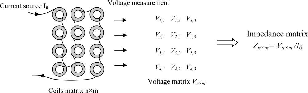
- - The synchronization of the supply and the measurement is not required for the electronic component.
- - The measurement of the coils impedance is carried throw the voltage measurement.
- - The incident electric field on the scan surface is uniform because the coils are connected in series, and this is independent of the work piece surface state.
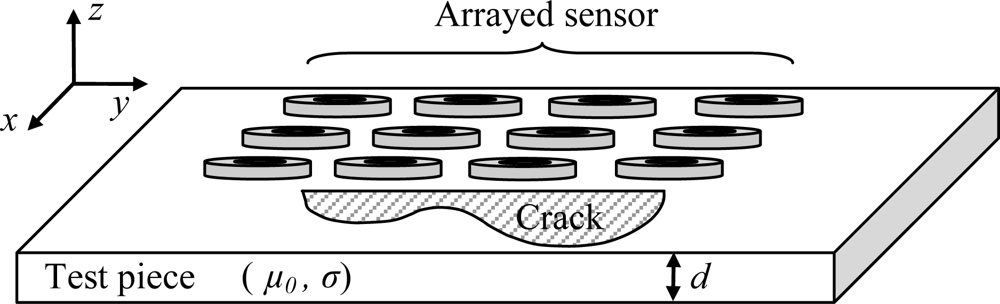
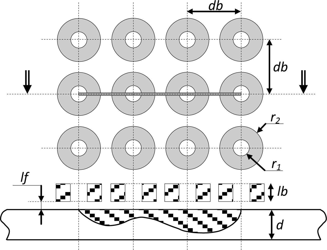
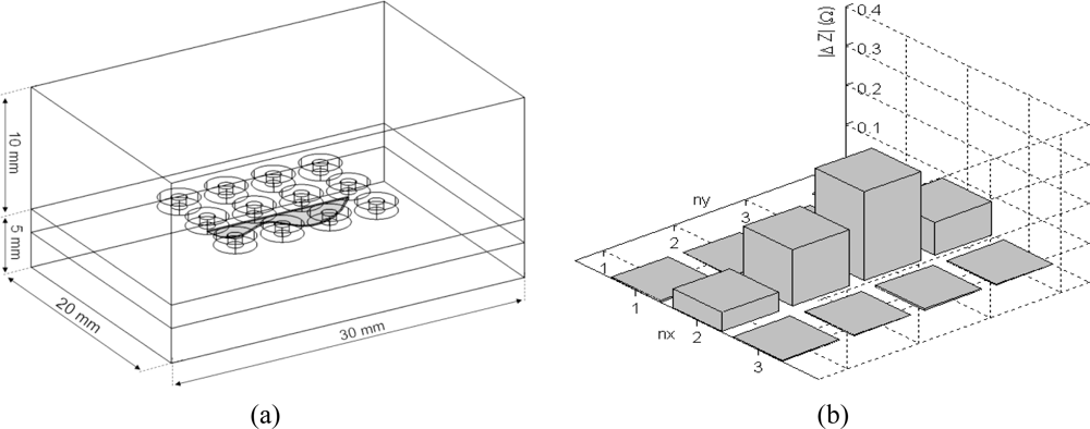
2. The Modeled System
3. Direct Problem Formulation
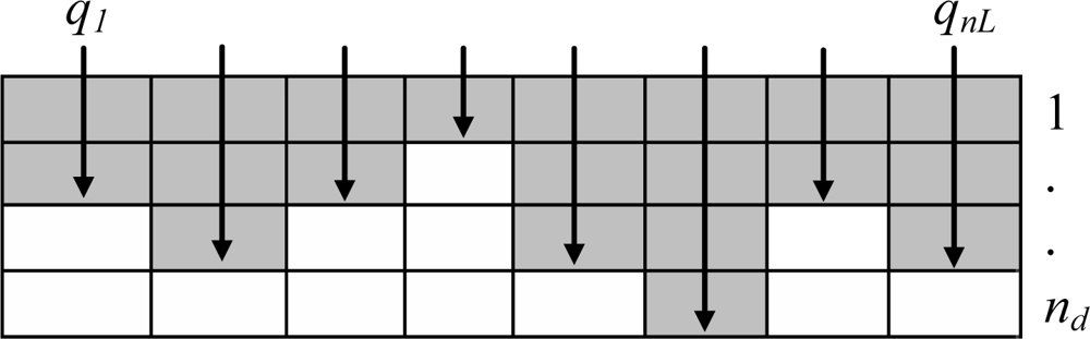
4. Inverse Problem
4.1. Reference data
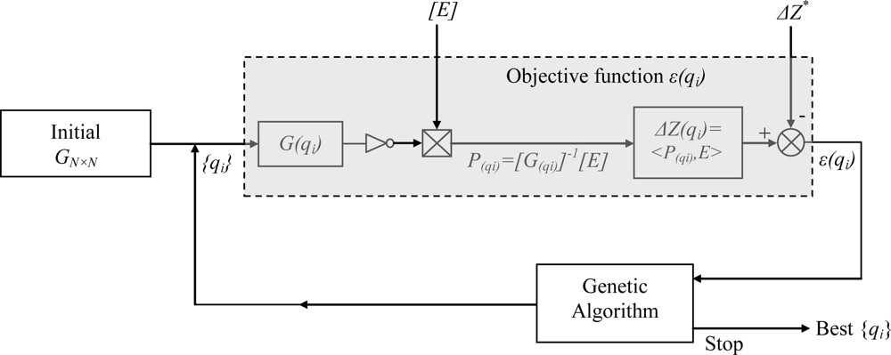
4.2. Inversion procedure
5. Conclusions
Acknowledgments
References
- Huang, H; Sakurai, N; Takagi, T; Uchimoto, T. Design of an eddy-current array probe for crack sizing in steam generator tubes. NDT&E Int 2003, 36, 515–522. [Google Scholar]
- Takagi, T; Uchimoto, T; Nagaya, Y; Huang, H; Endo, H. Design of eddy current camera for non-destructive testing. Proceedings of the SICE Annual Conference, Fukui, Japan, 4–6 August 2003; pp. 1711–1714.
- Grimberg, R; Udpa, L; Savin, A; Stengmann, R; Palihovici, V; Udpa, SS. 2D Eddy current sensor array. NDT&E Int 2006, 39, 264–271. [Google Scholar]
- Pavo, J; Miya, K. Reconstruction of crack shape by optimization using eddy current field measurement. IEEE Trans. Mag 1994, 30, 3407–3410. [Google Scholar]
- Pavo, J; Lesselier, D. Calculation of eddy current testing probe signal with global approximation. IEEE Trans. Mag 2006, 42, 1419–1422. [Google Scholar]
- Le Bihan, Y; Pavo, J; Bensetti, M; Marchand, C. Computational environment for the fast calculation of ECT probe signal by field decomposition. IEEE Trans. Mag 2006, 42, 1411–1414. [Google Scholar]
- Zaoui, A; Menana, H; Feliachi, M; Abdallah, M. Generalization of the ideal crack model for an arrayed eddy current sensor. IEEE Trans. Mag 2008, 44, 1638–1641. [Google Scholar]
- Zaoui, A; Feliachi, M; Abdallah, M; Djennah, M. Fast computing methodology for 3D arrayed sensor in eddy current Non Destructive Testing. Rev. Int. de Génie Électrique 2008, 11, 275–285. [Google Scholar]
- Dezhi, C; Shao, KR; Jianni, S; Weili, Y. Eddy current interaction with a thin-opening crack in a plate conductor. IEEE Trans. Magn 2000, 36, 1745–1749. [Google Scholar]
- Biro, O; Preis, K. On the use of the magnetic vector potential in the finite element analysis of three-dimensional eddy currents. IEEE Trans. Magn 1989, 25, 3145–3159. [Google Scholar]
- Geuzaine, C; Remacle, JF. Gmsh Reference Manual: A Finite Element Mesh Generator with Built-In Pre- And Post-Processing Facilities. Available online: www.geuz.org/gmsh (accessed on 17 September 2010).
- Yokose, Y; Cingoski, V; Yamashita, H. Genetic algorithms with assistant chromosomes for inverse shape optimization of electromagnetic devices. IEEE Trans. Magn 2000, 36, 1052–1056. [Google Scholar]
- Yokose, Y; Cingoski, V; Kaneda, K; Yamashita, H. Shape optimization of magnetic devices using genetic algorithms with dynamically adjustable parameters. IEEE Trans. Magn 1999, 35, 1686–1689. [Google Scholar]
- Haupt, RL; Werner, DH. Genetic Algorithms in Electromagnetics, 1st ed; Wiley and Sons Ltd.-IEEE Press: Hoboken, NJ, USA, 2007. [Google Scholar]


| Parameters | Values | |
|---|---|---|
| Frequency: | 300 kHz | |
| Coils: | Inner radius, r1 | 0.6 mm |
| Outer radius, r2 | 1.6 mm | |
| Height, lb | 0.8 mm | |
| Lift-off, lf | 0.5 mm | |
| Number of turns, N | 140 | |
| Distance between the coils, db | 4 mm | |
| Plate: | Thickness, d | 2 mm |
| Conductivity, σ | 1 MS/m | |
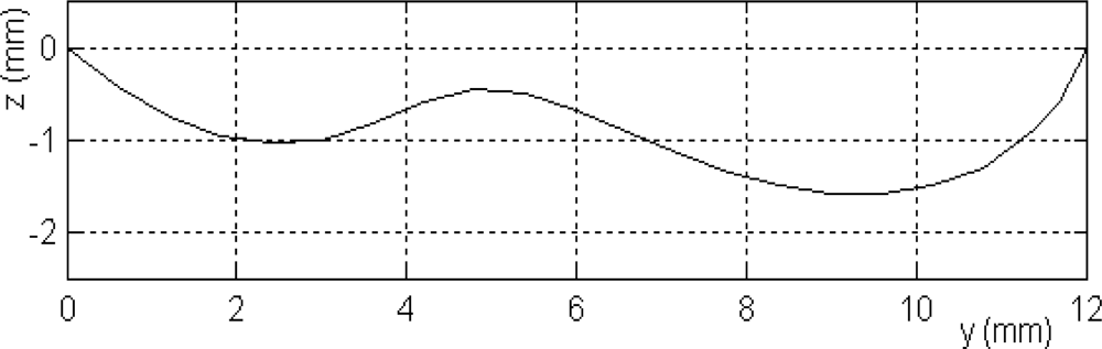
| Crack: | Length, L | 12 mm |
| Thickness | 0.2 mm | |
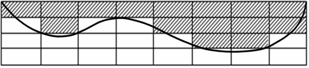
| Depth | Arbitrary shape (Figure 3) | |
| Parameters | Values |
|---|---|
| Population : | 64 |
| Crossover rates (Uniform) : | 0.8 |
| Mutation rates (Heuristic) : | 0.02 |
© 2010 by the authors; licensee MDPI, Basel, Switzerland. This article is an open access article distributed under the terms and conditions of the Creative Commons Attribution license (http://creativecommons.org/licenses/by/3.0/).
Share and Cite
Zaoui, A.; Menana, H.; Feliachi, M.; Berthiau, G. Inverse Problem in Nondestructive Testing Using Arrayed Eddy Current Sensors. Sensors 2010, 10, 8696-8704. https://doi.org/10.3390/s100908696
Zaoui A, Menana H, Feliachi M, Berthiau G. Inverse Problem in Nondestructive Testing Using Arrayed Eddy Current Sensors. Sensors. 2010; 10(9):8696-8704. https://doi.org/10.3390/s100908696
Chicago/Turabian StyleZaoui, Abdelhalim, Hocine Menana, Mouloud Feliachi, and Gérard Berthiau. 2010. "Inverse Problem in Nondestructive Testing Using Arrayed Eddy Current Sensors" Sensors 10, no. 9: 8696-8704. https://doi.org/10.3390/s100908696