Background Subtraction Approach Based on Independent Component Analysis

Abstract
:1. Introduction
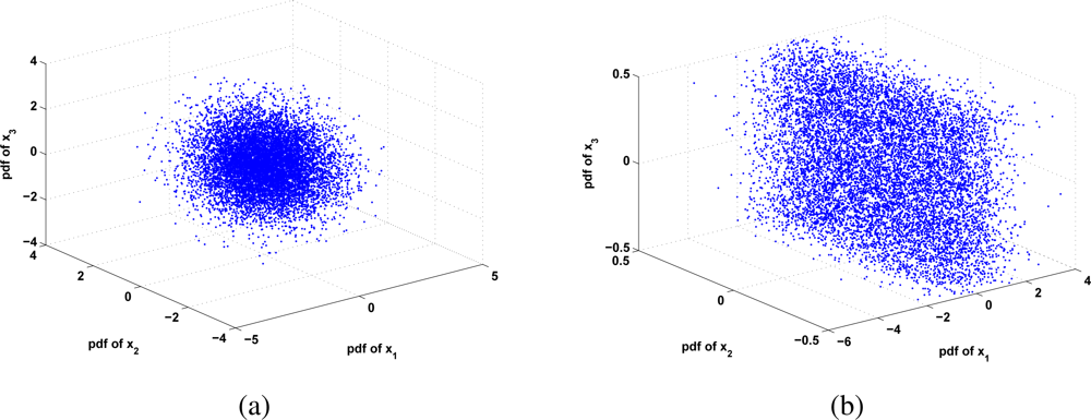
2. Background Model
3. Estimation of Unmixing Matrix
3.1. Image Preprocessing
3.2. Measure of Gaussianity
3.3. Parameter Estimation
- For each wi in W
- Choose initial (i.e., random) values weight for wi.
- Let .
- Let .
- If convergence is not achieved, go back to 1 (a).
- Continue with the next wi
3.4. The Background Gaussianity and Independent Component Separability
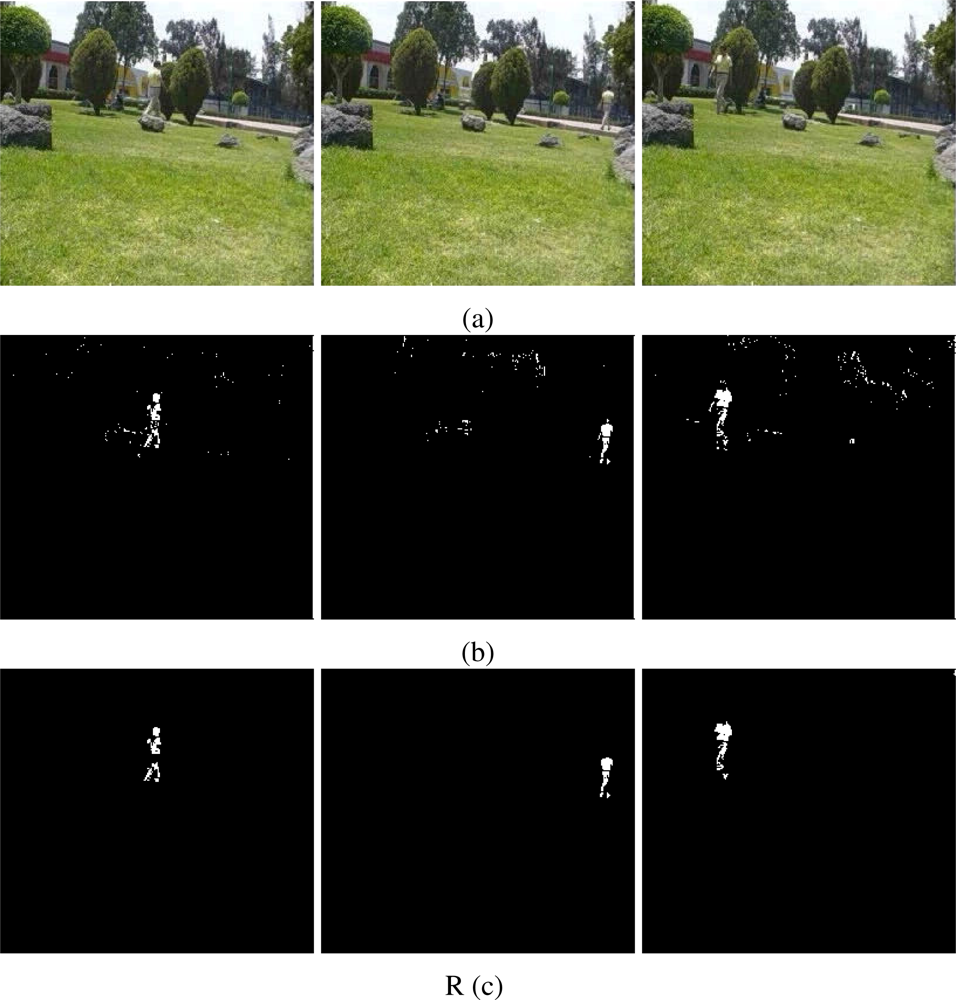
4. Motion Detection
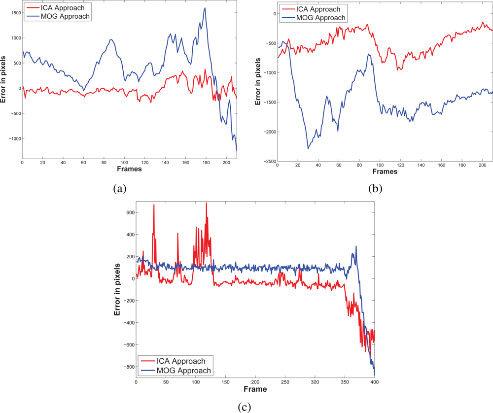
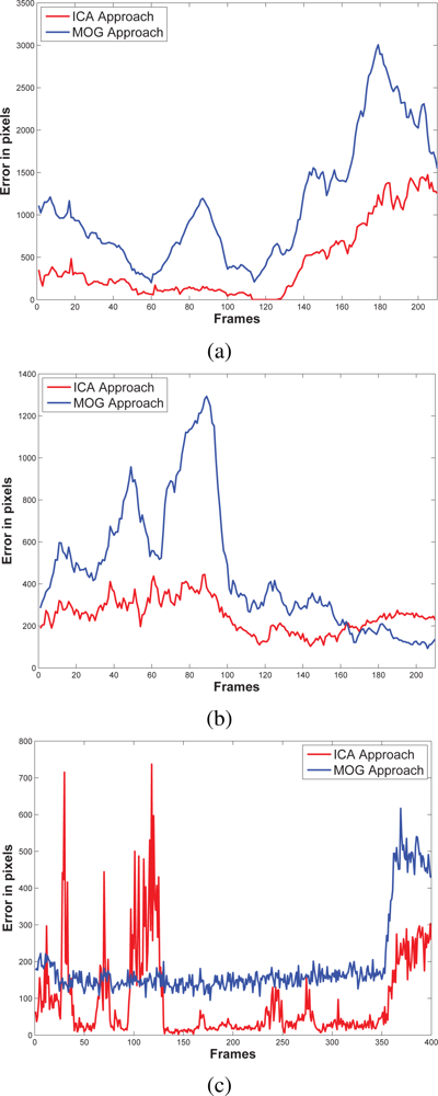
5. Experiments and Results
5.1. Implementation Issues
5.2. Experimental Model
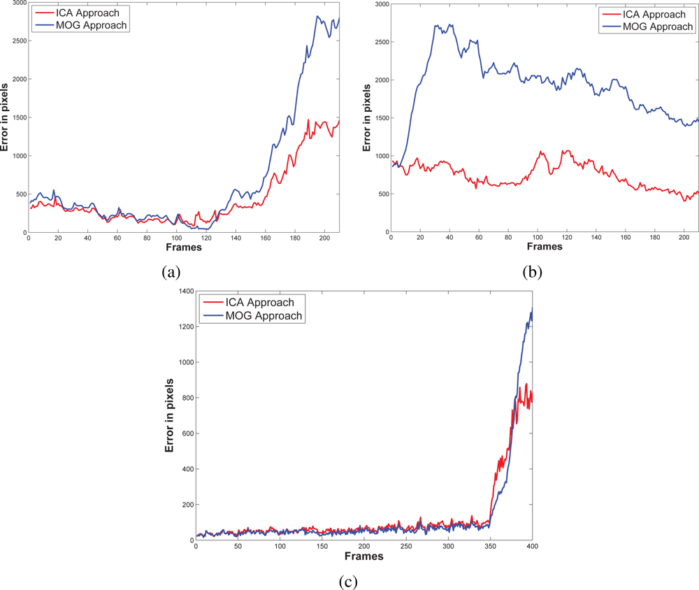
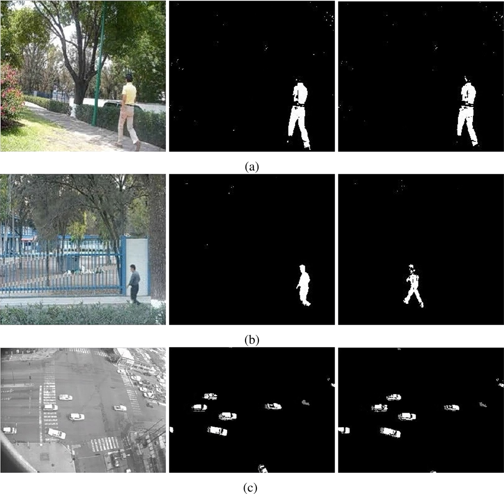
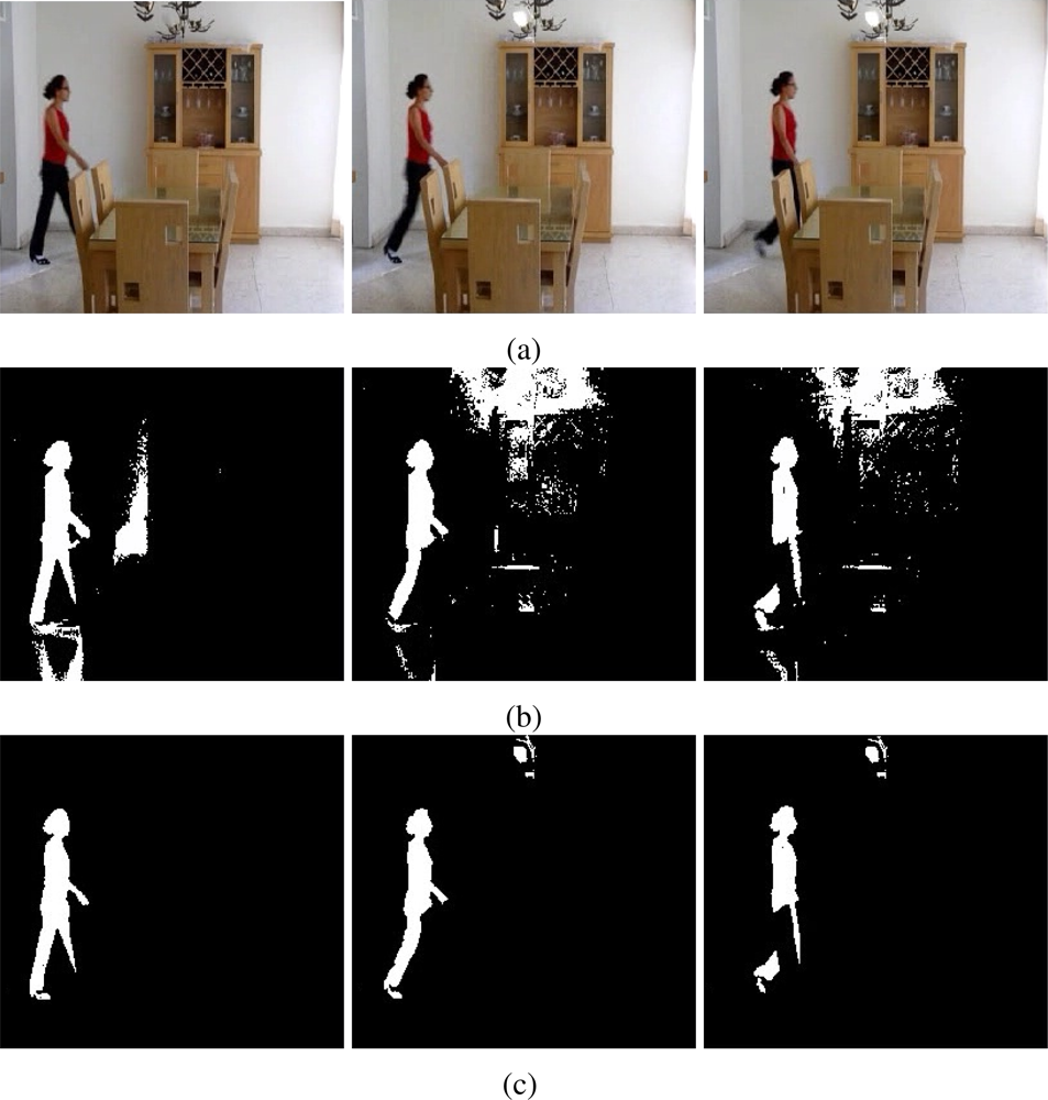
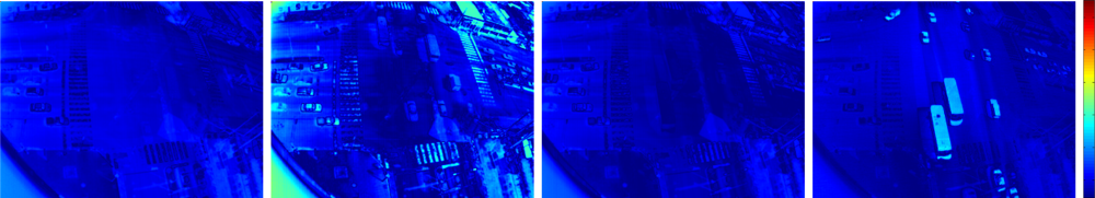
5.3. Results and Discussions
6. Conclusions
Acknowledgments
References
- Toyama, K.; Krumm, J.; Brumitt, B.; Meyers, B. Wallflower: Principles and Practice of Background Manteinance. Proceedings of IEEE Conference on Computer Vision and Pattern Recognition, Ft. Collins, CO, USA, June 23–25, 1999; 1, pp. 255–261.
- Horprasert, T.; Harwood, D.; Davis, L.S. A Robust Background Subtraction and Shadow Detection. Proceedings of Asian Conference on Computer Vision, Taipei, Taiwan, February 27–March 3, 2000.
- Stauffer, C.; Grimson, W. Adaptive Background Mixture Models for Real-Time Tracking. Proceedings of IEEE Conference on Computer Vision and Pattern Recognition, Ft. Collins, CO, USA, June 23–25, 1999; 2, pp. 252–259.
- Cheung, S.C.S.; Kamath, C. Robust Background Subtraction with Foreground Validation for Urban Traffic Video. EURASIP J. Appl. Signal Process 2005, 2005, 2330–2340. [Google Scholar]
- KaewTraKulPong, P.; Bowden, R. An Improved Adaptive Background Mixture Model for Real-time Tracking with Shadow Detection. Proceedings of the 2nd European Workshop on Advanced Video Based Surveillance Systems, London, UK, September 4, 2001; pp. 149–158.
- Elgammal, A.; Harwood, D.; Davis, L.S. Non-parametric Model for Background Subtraction. Proceedings of IEEE International Conference on Computer Vision, Kerkyra, Corfu, Greece, September 20–25, 1999.
- Oliver, N.M.; Rosario, B.; Pentland, A.P. A Bayesian Computer Vision System for Modeling Human Interactions. IEEE Trans. Pattern Anal. Mach. Intell 2000, 22, 831–843. [Google Scholar]
- Shaw, P.J.A. Multivariate Statistics for the Environmental Sciences; Hodder-Arnold: London, UK, 2003. [Google Scholar]
- Rymel, J.; Renno, J.; Greenhill, D.; Orwell, J.; Jones, G. Adaptive Eigen-Backgrounds for Object Detection. Proceedings of IEEE International Conference on Image Processing, Singapore, October 24–27, 2004; 3, pp. 1847–1850.
- Han, B.; Comaniciu, D.; Davis, L. Sequential Kernel Density Approximation through Mode Propagation: Applications to Background Modeling. Proceedings of Asian Conference on Computer Vision, Jeju Island, Korea, January 2004.
- Tang, Z.; Miao, Z. Fast Background Subtraction and Shadow Elimination Using Improved Gaussian Mixture Model. Proceedings of the 6th IEEE International Workshop on Haptic, Audio and Visual Environments and Games, Ottawa, ON, Canada, October 12–14, 2007; pp. 38–41.
- Zhou, D.; Zhang, H.; Ray, N. Texture based Background Subtraction. Proceedings of International Conference on Information and Automation, Zhangjiajie, Hunan, China, June 20–23, 2008; pp. 601–605.
- Tsai, D.M.; Lai, S.C. Independent Component Analysis-Based Background Subtraction for Indoor Surveillance. IEEE Trans. Image Process 2009, 18, 158–167. [Google Scholar]
- Hyvarinen, A. Survey on Independent Component Analysis. Neural Comput. Surv 1999, 2, 94–128. [Google Scholar]
- Comon, P. Independent Component Analysis—A New Concept? Signal Process 1994, 36, 287–314. [Google Scholar]
- Suli, E.; Mayers, D. An Introduction to Numerical Analysis; Cambridge University Press: Cambridge, UK, 2003. [Google Scholar]
- The University of Reading. Performance Evaluation of Tracking and Surveillance (PETS). Internet, ftp://ftp.pets.rdg.ac.uk/pub/PETS2001/, 2001. The University of Reading, UK.
- Thirde, D.; Ferryman, J.; Crowley, J.L. Performance Evaluation of Tracking and Surveillance (PETS). Available online: http://pets2006.net/ (accessed on 5 February 2010).
- Kalman, R. A New Approach to Linear Liltering and Prediction Problems. J. Basic Eng 1960, 82, 35–45. [Google Scholar]
- Dempster, A.; Laird, N.; Rubin, D. Maximum Likelihood from Incomplete Data via the EM Algorithm. JR Statist. Soc 1977, 39, 1–38. [Google Scholar]
- Hyvainen, A. Fast and Robust Fixed-Point Algorithms for Independent Component Analysis. IEEE Trans. Neural Networks 1999, 10, 626–634. [Google Scholar]
- Harry, L.; Papadimitrou, C. Elements of the Theory of Computation; Prentice Hall: Upper Saddle River, NJ, USA, 1988. [Google Scholar]
- Russell, S.; Norvig, P. Artificial Intelligence: A Modern Approach; Prentice Hall: Upper Saddle River, NJ, USA, 2003. [Google Scholar]
- Salembier, P.; Serra, J. Flat Zones Filtering, Connected Operators and Filters by Reconstruction. IEEE Trans. Image Process 1995, 4, 1153–1160. [Google Scholar]
- Bao, P.; Zhang, L. Noise Reduction for Multi-scale Resonance Images via Adaptive Multiscale Products Thresholding. IEEE Trans. Med. Imaging 2003, 2, 1089–1099. [Google Scholar]
- Pless, R.; Larson, J.; Siebers, S.; Westover, B. Evaluation of Local Models of Dynamic Backgrounds. Proceedings of IEEE Computer Society Conference on Computer Vision and Pattern Recognition, Madison, WI, USA, June 16–22, 2003; 2, pp. 73–78.
- Herrero, S.; Bescós, J. Background Subtraction Techniques: Systematic Evaluation and Comparative Analysis. In Advanced Concepts for Intelligent Vision Systems; Springer Verlag: Berlin, Germany, 2009. [Google Scholar]
- Papoulis, A. Probability, Random Variables, and Stochastic Processes; McGraw-Hill: New York, NY, USA, 1991. [Google Scholar]
- Duda, R.O.; Hart, P.E.; Stork, D.G. Pattern Classification; Wiley-Interscience: Malden, MA, USA, 2000. [Google Scholar]
A Motion Detection and PCA approach


| No. | Estimator |
|---|---|
| 1 | E(ϒ) = Ĩ(x) where each |
| 2 | E(ϒ) = Ĩ(x) where each Ĩ(x) = median {Ii∈ϒ(x)} |
| 3 | E(ϒ) = μx where each Ĩ(x) ∼ G(μx, σx) |
| No. | Function |
|---|---|
| 1 | |
| 2 | |
| 3 | G(u) = u3 |
| No. | Place | Source | Num. Img.1 | bf Num. Train. 2 |
|---|---|---|---|---|
| 1 | Train Station | PETS 2007 | 300 | 100 |
| 2 | Train Station | PETS 2007 | 300 | 100 |
| 3 | Outdoors Park | PETS 2001 | 500 | 100 |
© 2010 by the authors; licensee MDPI, Basel, Switzerland. This article is an open access article distributed under the terms and conditions of the Creative Commons Attribution license (http://creativecommons.org/licenses/by/3.0/).
Share and Cite
Jiménez-Hernández, H. Background Subtraction Approach Based on Independent Component Analysis. Sensors 2010, 10, 6092-6114. https://doi.org/10.3390/s100606092
Jiménez-Hernández H. Background Subtraction Approach Based on Independent Component Analysis. Sensors. 2010; 10(6):6092-6114. https://doi.org/10.3390/s100606092
Chicago/Turabian StyleJiménez-Hernández, Hugo. 2010. "Background Subtraction Approach Based on Independent Component Analysis" Sensors 10, no. 6: 6092-6114. https://doi.org/10.3390/s100606092
APA StyleJiménez-Hernández, H. (2010). Background Subtraction Approach Based on Independent Component Analysis. Sensors, 10(6), 6092-6114. https://doi.org/10.3390/s100606092