Arrhythmia ECG Noise Reduction by Ensemble Empirical Mode Decomposition

Abstract
:1. Introduction
2. EMD and EEMD algorithm
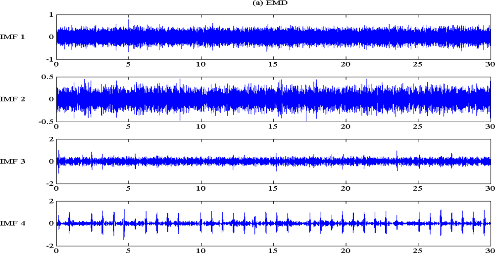
2.1. EMD
- Identify all the extrema (maxima and minima) of the signal, x(s).
- Generate the upper and lower envelope by the cubic spline interpolation of the extrema point developed in step (1).
- Calculate the mean function of the upper and lower envelope, m(t).
- Calculate the difference signal d(t) = x(t)−m(t).
- If d(t) becomes a zero-mean process, then the iteration stop and d(t) is an IMF1, named c1(t); otherwise, go to step (1) and replace x(t) with d(t).
- Calculate the residue signal r(t) = x(t)−c1(t).
- Repeat the procedure from steps (1) to (6) to obtain IMF2, named c2(t). To obtain cn(t), continue steps (1)–(6) after n iterations. The process is stopped when the final residual signal r(t) is obtained as a monotonic function.
2.2. EEMD
- Add a white noise series n(t) to the targeted signal, named x1(t) in the following description, and x2(t)=x1(t)+n(t).
- Decompose the data x2(t) by EMD algorithm, as described in Section 2.1.
- Repeat Steps (1) and (2) until the trial numbers, each time with different added white noise series of the same power at each time. The new IMF combination Cij(t) is achieved, where i is the iteration number and j is the IMF scale.
- Estimate the mean (ensemble) of the final IMF of the decompositions as the desired output:where ni denotes the trial numbers.
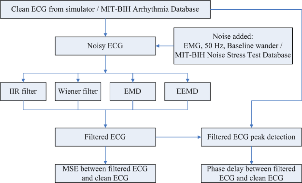
3. Method
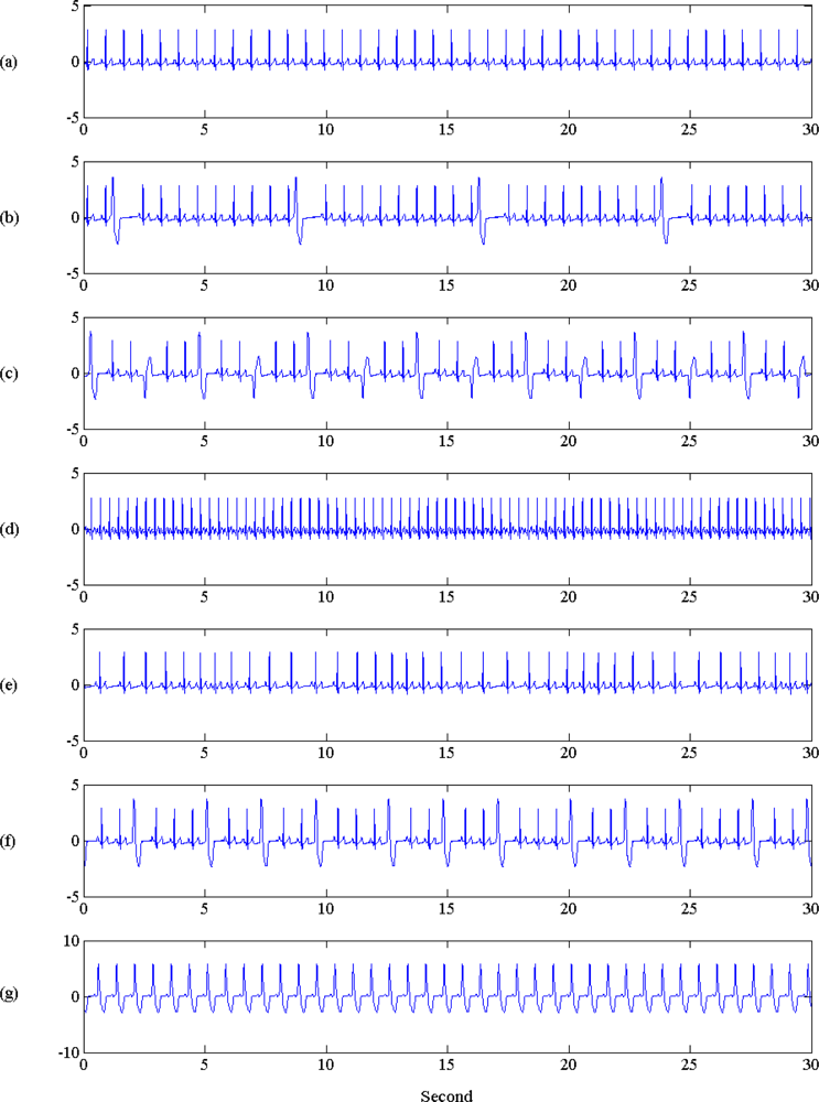
3.1. Simulated Arrhythmia ECG and Noise Data
A. Clean synthetic ECG signal:
B. Real ECG database
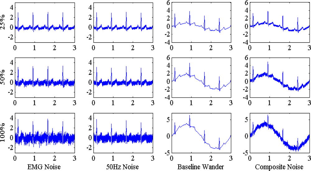
C. Synthetic noises:
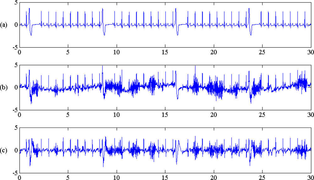
- EMG noise: EMG noise was model by a random number with normal distribution, originally manipulated with the Matlab code randn.m. The maximum EMG noise level was the scaling of random sequence and the multiplication to Vpp with reduced ratio of 1/8. EMG noise sequence was denoted as N1(t).
- Power line noise: Power line interference was modeled by 50 Hz sinusoidal function with multiplication on amplitude derived with Matlab code rand.m. The maximum 50 Hz noise level was the scaling of random sequence and the multiplication to Vpp with reduced ratio of 1/4. 50 Hz noise sequence was denoted as N2(t).
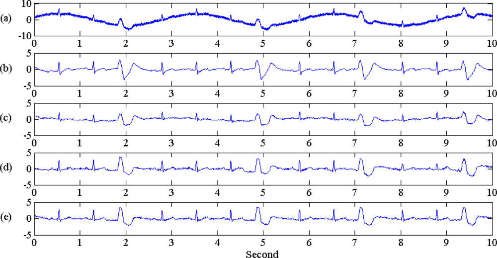
- Baseline wander: Baseline wander was model by a Baseline wander a 0.333 Hz sinusoidal function. The maximum noise level was the same amplitude scale with Vpp. Baseline wander was denoted as N3(t).
- Composite noise: Composite noise was the combination of the above three noise with the following relation:
D. Real noise database
3.2. EMD/EEMD Based Filtering Algorithm
3.3. Wiener Filter
3.4. Traditional IIR Filter
3.5. Filtering Performance Index
4. Results:
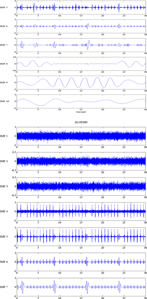
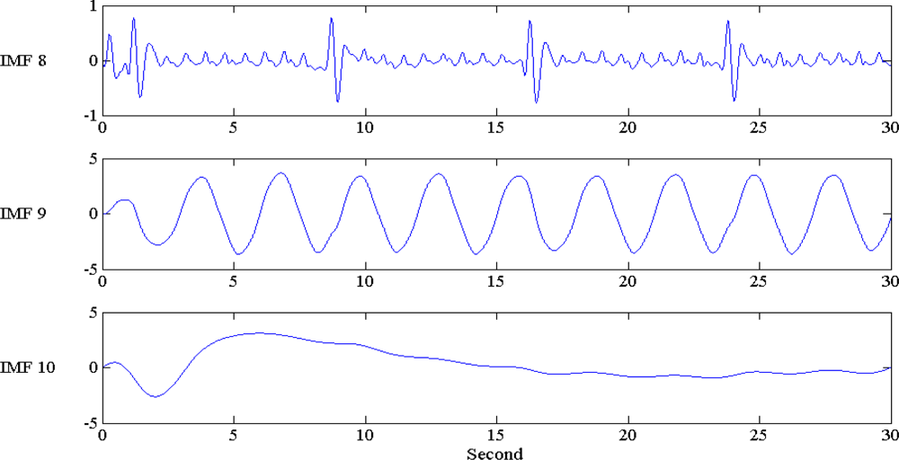
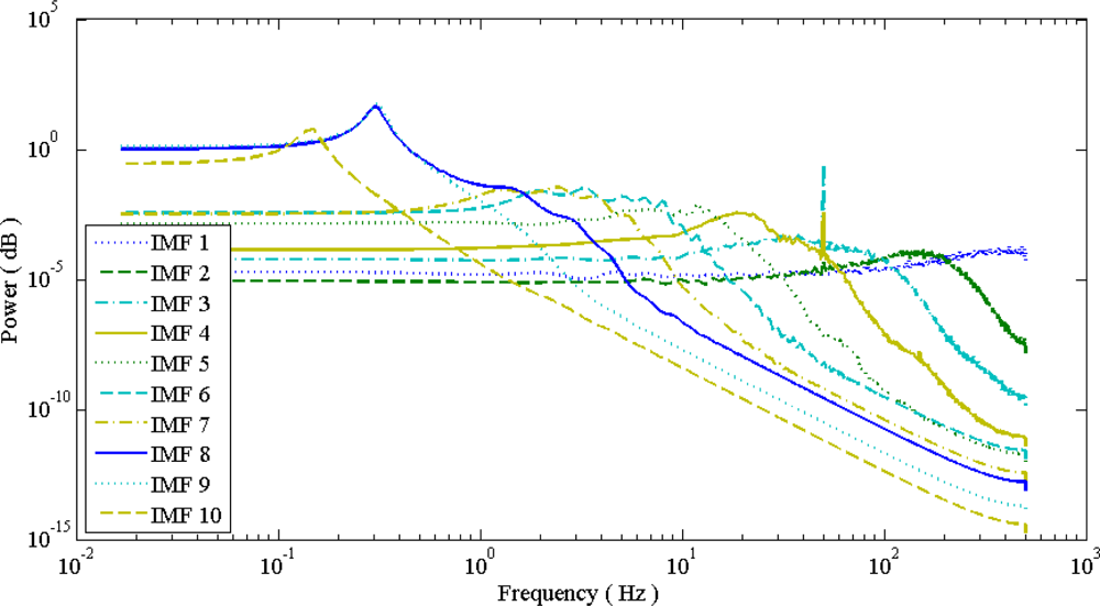
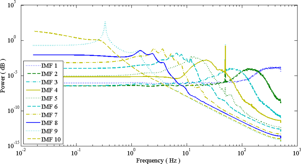
4.1. EMD and EEMD Decomposition:
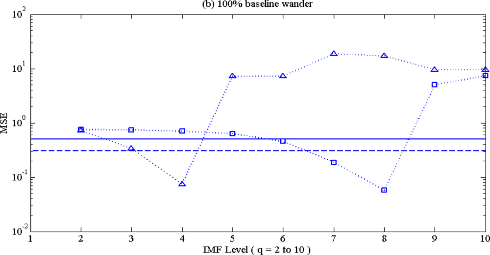
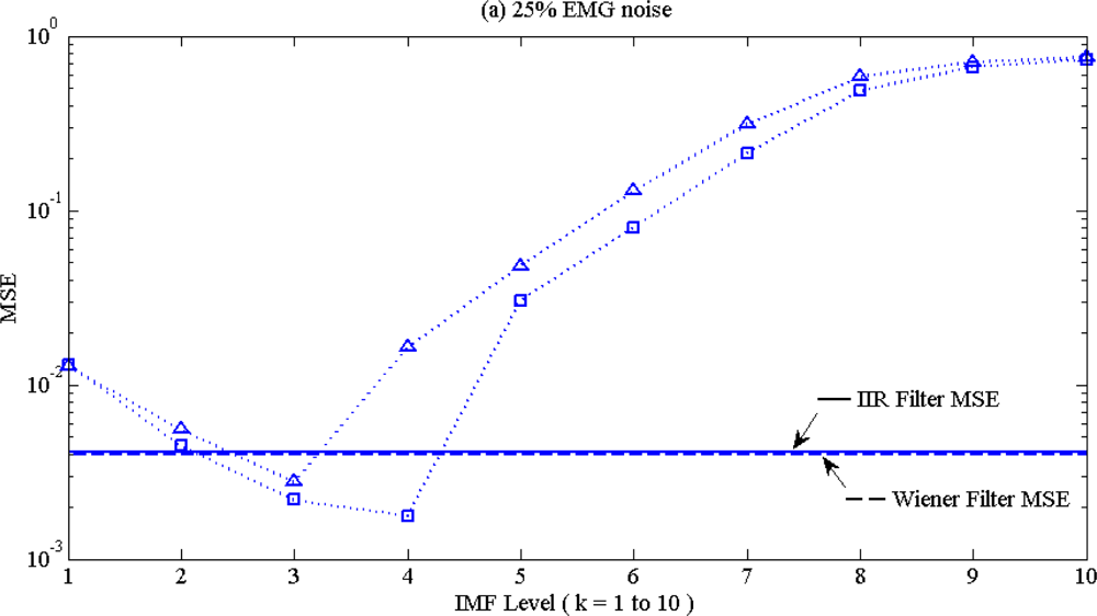
4.2. MSE Performance:
5. Discussion:
6. Conclusions
Acknowledgments
References
- Huang, N.E.; Shen, Z.; Long, S.R.; Wu, M.C.; Shih, H.H.; Zheng, Q.; Yen, N.C.; Tung, C.C.; Liu, H.H. The empirical mode decomposition and the Hilbert spectrum for nonlinear and non-stationary time series analysis. Proc. Roy. Soc. Lond 1998, 454, 903–995. [Google Scholar]
- Flandrin, P.; Rilling, G.; Goncalves, P. Empirical mode decomposition as a filter bank. IEEE Signal Process. Lett 2004, 11, 112–114. [Google Scholar]
- Li, D.; Liang, Z.; Voss, L.J.; Sleigh, J.W. Analysis of depth of anesthesia with Hilbert-Huang spectral entropy. Clin. Neurophysiol 2008, 119, 2465–2475. [Google Scholar]
- Salisbury, J.I.; Sun, Y. Rapid screening test for sleep apnea using a nonlinear and nonstationary signal processing technique. Med. Eng. Phys 2007, 29, 336–343. [Google Scholar]
- Balocchi, R.; Menicucci, D.; Santarcangelo, E.; Sebastiani, L.; Gemigani, A.; Ghelarducci, B.; Varanini, M. Deriving the respiratory sinus arrhythmia from the heartbeat time series using empirical mode decomposition. Chaos Solitons Fractals 2004, 20, 171–177. [Google Scholar]
- Weng, B.; Blanco-Velasco, M.; Barner, K.E. ECG Denoising based on the Empirical Mode Decomposition. Conf. Proc. IEEE. Eng. Med. Biol. Soc 2006, 1, 1–4. [Google Scholar]
- Lu, Y.; Yan, J.Y.; Yam, Y. Model-based ECG Denoising Using Empirical Mode Decomposition. Conf. Proc. IEEE BIBM 2009, 2009, 191–196. [Google Scholar]
- Pan, N.; I, V. M.; Un, M.P.; Hang, P.S. Accurate Removal of Baseline Wander in ECG Using Empirical Mode Decomposition. Conf. Proc. NFSI ICFBI 2007, 2007, 177–180. [Google Scholar]
- Li, N.Q.; Li, P. An Improved Algorithm Based on EMD-Wavelet for ECG Signal De-noising. Proceedings of International Joint Conference on Computational Sciences and Optimization 2009, Sanya, Hainan, China, 24–26 April 2009; 1.
- Blanco-Velasco, M.; Weng, B.; Barner, K.E. ECG signal denoising and baseline wander correction based on the empirical mode decomposition. Comput. Biol. Med 2008, 38, 1–13. [Google Scholar]
- Nimunkar, A.J.; Tompkins, W.J. EMD-based 60-Hz noise filtering of the ECG. Conf. Proc. IEEE Eng. Med. Biol. Soc 2007, 2007, 1904–1907. [Google Scholar]
- Wu, Z.; Huang, N.E. A study of the characteristics of white noise using the empirical mode decomposition method. Proc. Roy. Soc. London. A 2004, 460, 1597–1611. [Google Scholar]
- Wu, Z.; Huang, N.E. Ensemble empirical mode decomposition: a noise-assisted data analysis method. Adv. Adapt. Data. Anal 2009, 1, 1–41. [Google Scholar]
- Chen, L.; Li, X.; Li, X.B.; Huang, Z.Y. Signal extraction using ensemble empirical mode decomposition and sparsity in pipeline magnetic flux leakage nondestructive evaluation. Rev. Sci. Instrum 2009, 80, 025105. [Google Scholar]
- Abdulhay, E.; Gumery, P.Y.; Fontecave, J.; Baconnier, P. Cardiogenic oscillations extraction in inductive plethysmography: Ensemble empirical mode decomposition. Conf. Proc. IEEE Eng. Med. Biol. Soc 2009, 1, 2240–2243. [Google Scholar]
- Rheinberger, K.; Steinberger, T.; Unterkofler, K.; Baubin, M.; Klotz, A.; Amann, A. Removal of CPR artifacts from the ventricular fibrillation ECG by adaptive regression on lagged reference signals. IEEE Trans. Biomed. Eng 2008, 55, 130–137. [Google Scholar]
- Husøy, J.H.; Eilevstjønn, J.; Eftestøl, T.; Aase, S.O.; Myklebust, H.; Steen, P.A. Removal of cardiopulmonary resuscitation artifacts from human ECG using an efficient matching pursuit-like algorithm. IEEE Trans. Biomed. Eng 2002, 49, 1287–1298. [Google Scholar]
- Irusta, U.; Ruiz, J.; de Gauna, S.R.; Eftestøl, T.; Kramer-Johansen, J. A least mean-square filter for the estimation of the cardiopulmonary resuscitation artifact based on the frequency of the compressions. IEEE Trans. Biomed. Eng 2009, 56, 1052–1062. [Google Scholar]
- Wu, Y.; Rangayyan, R.M.; Zhou, Y.; Ng, S.C. Filtering electrocardiographic signals using an unbiased and normalized adaptive noise reduction system. Med. Eng. Phys 2009, 31, 17–26. [Google Scholar]
- Lander, P.; Berbari, E.J. Time-frequency plane Wiener filtering of the high-resolution ECG: background and time-frequency representations. IEEE Trans. Biomed. Eng 1997, 44, 247–2455. [Google Scholar]
- Goldberger, A.L.; Amaral, L.A.N.; Glass, L.; Hausdorff, J.M.; Ivanov, P.C.; Mark, R.G.; Mietus, J.E.; Moody, G.B.; Peng, C.K.; Stanley, H.E. PhysioBank, PhysioToolkit, and PhysioNet: components of a new research resourcefor complex physiologic signals. Circulation 2000, 101, E 215–E 220. [Google Scholar]
- Friesen, G.M.; Jannett, T.C.; Jadallah, M.A.; Yates, S.L.; Quint, S.R.; Nagle, H.T. A comparison of the noise sensitivity of nine QRS detection algorithms. IEEE Trans. Biomed. Eng 1990, 37, 85–98. [Google Scholar]
- Moody, G.B.; Muldrow, W.E.; Mark, R.G. A noise stress test for arrhythmia detectors. Comput. Cardiol 1984, 11, 381–384. [Google Scholar]
- Chang, K.M.; Liu, S.H. Gaussian Noise Filtering from ECG by Wiener Filter and Ensemble Empirical Mode Decomposition. J. Sign. Process. Syst 2010. [Google Scholar] [CrossRef]
- Saeed, V.V. Advanced Digital Signal Processing and Noise Reduction, 3rd. ed; Wiley: New York, NY, USA, 2006. [Google Scholar]


| Noise type | Noise percentage | IIR | Wiener | EMD (IMF level) | EEMD (IMF level) |
|---|---|---|---|---|---|
| EMG (* E-3) | 25 % | 4.1 | 4.0 | 2.8 (k = 3) | 1.8 (k = 4) |
| 50% | 6.6 | 12.3 | 11.1 (k = 4) | 4.6 (k = 4) | |
| 100% | 18.1 | 34.4 | 24.6 (k = 4) | 18.1 (k = 4) | |
| 50 Hz (* E-3) | 25 % | 3.3 | 1.0 | 7.2 (k = 2) | 2.0 (k = 4) |
| 50% | 3.8 | 3.0 | 11.9 (k = 4) | 3.0 (k = 4) | |
| 100% | 5.7 | 9.4 | 10.7 (k = 4) | 5.1 (k = 4) | |
| Baseline (* E-2) | 25 % | 49.5 | 10.1 | 3.0 (q = 5) | 2.3 (q = 9) |
| 50% | 49.7 | 18.4 | 8.5 (q = 5) | 4.8 (q = 8) | |
| 100% | 50.5 | 30.4 | 7.4 (q = 4) | 5.7 (q = 8) | |
| Composite (* E-2) | 25 % | 52.6 | 10.3 | 8.5 (k = 3, q = 8) | 2.3 (k = 4, q = 9) |
| 50% | 52.8 | 18.8 | 5.5 (k = 3, q = 8) | 5.0 (k = 4, q = 8) | |
| 100% | 54.2 | 31.7 | 19.5 (k = 4, q = 7) | 6.6 (k = 4, q = 8) | |
| “em”(* E-2) | 100% | 49.1 | 19.6 | 19.3 (k = 1, q = 5) | 16.3 (k = 4, q = 7) |
| “ma” (* E-2) | 100% | 36.1 | 10.7 | 13.3 (k = 3, q = 7) | 8.5 (k = 5, q = 9) |
| “bw” (* E-2) | 100 % | 23.1 | 6.9 | 2.7 (k = 1, q = 7) | 1.5 (k = 4, q = 9) |
| Noise type | Noise percentage | IIR | Wiener | EMD | EEMD |
|---|---|---|---|---|---|
| EMG (* E-3) | 25 % | 9.5 | 19.1 | 19.7 | 18.6 |
| 50% | 12.0 | 65.1 | 75.8 | 67.7 | |
| 100% | 44.6 | 140.5 | 172.3 | 164.4 | |
| 50Hz (* E-3) | 25 % | 8.6 | 2.1 | 8.4 | 3.4 |
| 50% | 9.1 | 26.2 | 41.4 | 27.8 | |
| 100% | 12.2 | 11.9 | 19.2 | 12.0 | |
| Baseline (* E-2) | 25 % | 53.4 | 9.3 | 2.4 | 1.6 |
| 50% | 53.7 | 19.4 | 7.0 | 4.5 | |
| 100% | 54.5 | 34.5 | 7.5 | 6.1 | |
| Composite (* E-2) | 25 % | 57.7 | 9.5 | 5.7 | 1.6 |
| 50% | 58.2 | 20.3 | 5.1 | 4.8 | |
| 100% | 58.9 | 37.7 | 18.6 | 7.1 | |
| ‘em’(* E-2) | 100% | 63.6 | 33.4 | 38.7 | 34.5 |
| ‘ma’ (* E-2) | 100% | 54.9 | 41.4 | 55.7 | 50.8 |
| ‘bw’ (* E-2) | 100 % | 22.9 | 34.7 | 42.9 | 41.7 |
| Signal | Noise | IIR | Wiener | EMD | EEMD |
|---|---|---|---|---|---|
| 101 (* E-2) | em | 14.7 | 6.7 | 8.6 | 6.5 |
| ma | 6.0 | 2.4 | 3.6 | 2.2 | |
| bw | 4.1 | 1.6 | 1.0 | 0.7 | |
| 102 (* E-2) | em | 18.2 | 7.5 | 10.9 | 7.9 |
| ma | 9.5 | 2.3 | 3.2 | 1.9 | |
| bw | 7.6 | 1.9 | 1.3 | 0.8 | |
| 103 (* E-2) | em | 13.7 | 6.2 | 7.3 | 5.7 |
| ma | 5.0 | 2.4 | 3.7 | 2.8 | |
| bw | 3.1 | 1.3 | 1.0 | 0.6 |
© 2010 by the authors; licensee MDPI, Basel, Switzerland. This article is an open access article distributed under the terms and conditions of the Creative Commons Attribution license (http://creativecommons.org/licenses/by/3.0/).
Share and Cite
Chang, K.-M. Arrhythmia ECG Noise Reduction by Ensemble Empirical Mode Decomposition. Sensors 2010, 10, 6063-6080. https://doi.org/10.3390/s100606063
Chang K-M. Arrhythmia ECG Noise Reduction by Ensemble Empirical Mode Decomposition. Sensors. 2010; 10(6):6063-6080. https://doi.org/10.3390/s100606063
Chicago/Turabian StyleChang, Kang-Ming. 2010. "Arrhythmia ECG Noise Reduction by Ensemble Empirical Mode Decomposition" Sensors 10, no. 6: 6063-6080. https://doi.org/10.3390/s100606063