Integration of a Multi-Camera Vision System and Strapdown Inertial Navigation System (SDINS) with a Modified Kalman Filter


Abstract
:1. Introduction
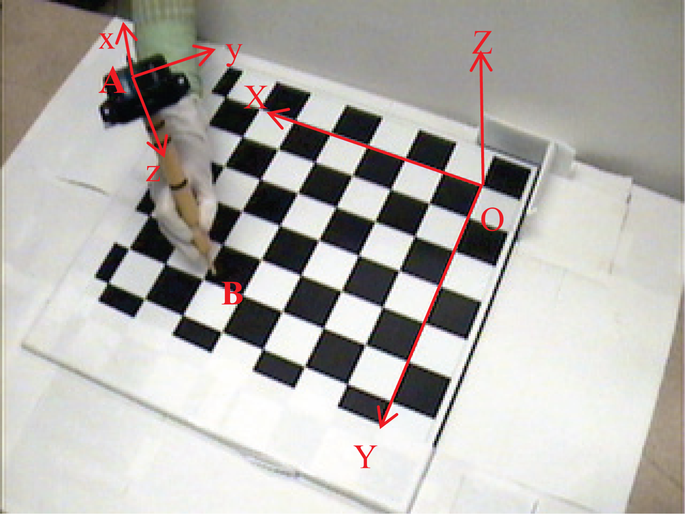
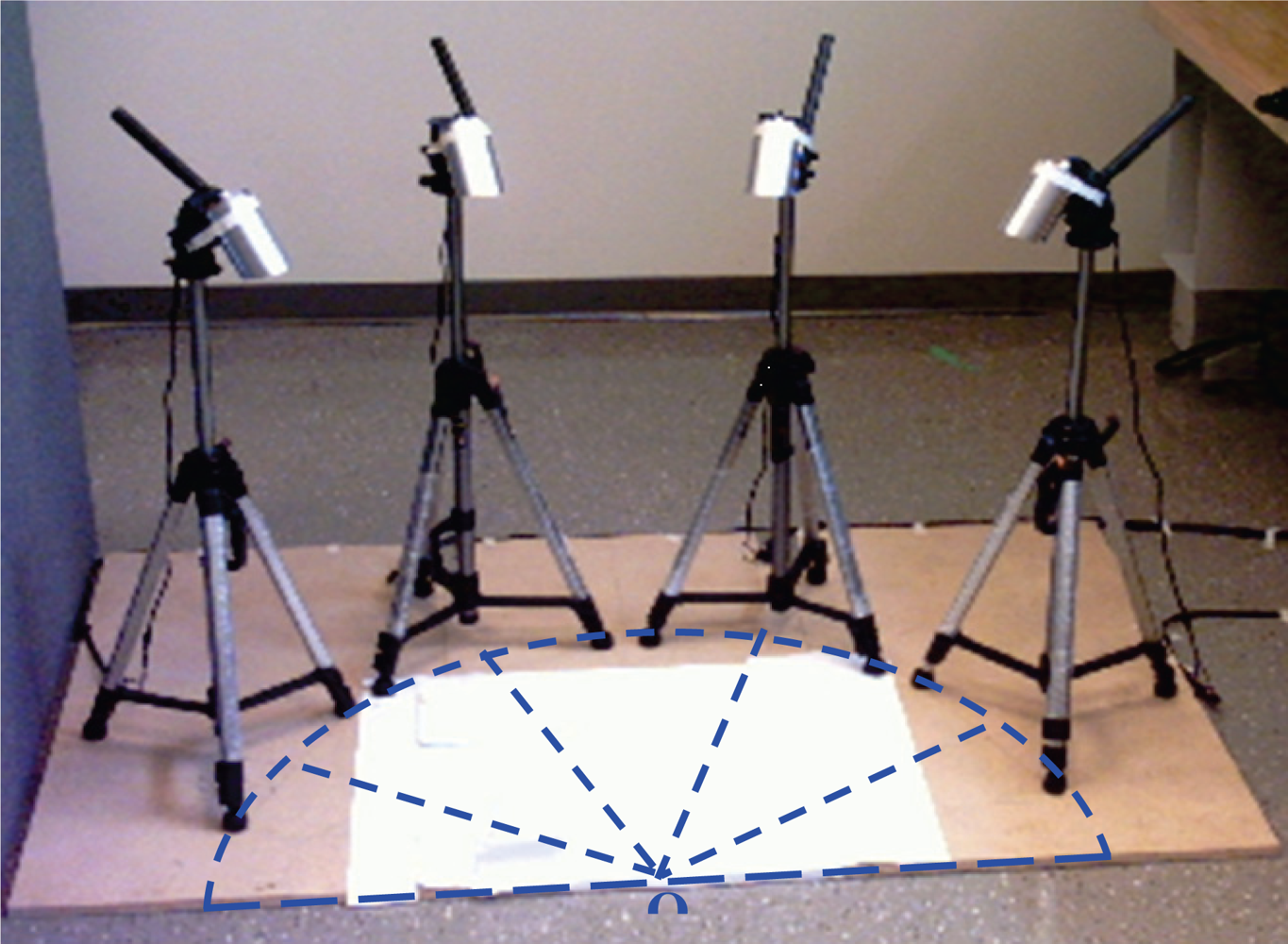
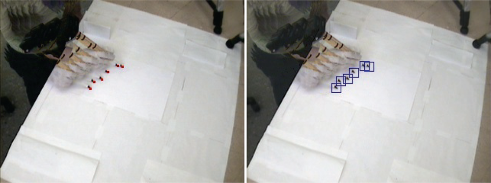
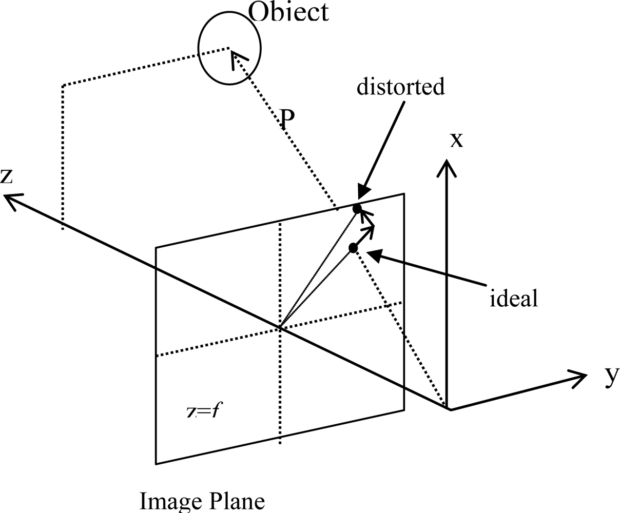
3. Vision System
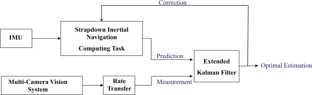
4. Modified Kalman Filter
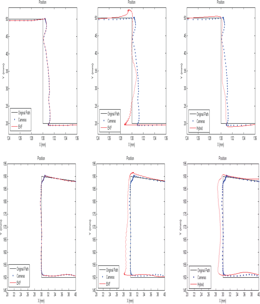
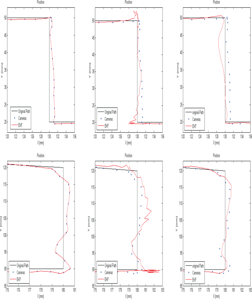
5. Experimental Results
6. Conclusions
References
- Farrell, J.; Barth, M. Global Positioning System and Inertial Navigation; McGraw-Hill: New York, NY, USA, 1999; p. 145. [Google Scholar]
- Grewal, M.; Weill, L.R.; Andrews, A.P. Global Positioning Systems, Inertial Navigation, and Integration, 2nd ed; John Wiley & Sons: Hoboken, NJ, USA, 2007. [Google Scholar]
- Foxlin, E.; Naimark, L. VIS-Tracker: A Wearable Vision-Inertial Self-Tracker. Proceedings of IEEE Virtual Reality Conference, Los Angeles, CA, USA, March 2003; pp. 199–206.
- Parnian, N.; Golnaraghi, F. Integration of Vision and Inertial Sensors for Industrial Tools Tracking. Sens. Rev 2007, 27, 132–141. [Google Scholar]
- Parnian, N.; Golnaraghi, F. A low-Cost Hybrid SDINS/Multi-Camera Vision System for a Hand-Held Tool Positioning. Proceedings of 2008 IEEE/ION Position, Location and Navigation Symposium, Monterey, CA, USA, May 6–8, 2008; pp. 489–496.
- Ernest, P.; Mazl, R.; Preucil, L. Train Locator Using Inertial Sensors and Odometer. Proceedings of IEEE Intelligent Vehicles Symposium, Parma, Italy, June 2004; pp. 860–865.
- Pingyuan, C.; Tianlai, X. Data Fusion Algorithm for INS/GPS/Odometer Integrated Navigation. Proceedings of IEEE Conference on Industrial Electronics and Applications, Harbin, China, May 2007; pp. 1893–1897.
- Abuhadrous, I.; Nashashibi, F.; Laurgeau, C. 3D Land Vehicle Localization: A Real-time Multi-Sensor Data Fusion Approach using RTMAPS. Proceedings of the 11th International Conference on Advanced Robotics, Coimbra, Portugal, June 30–July 3, 2003; pp. 71–76.
- Bian, H.; Jin, Z.; Tian, W. Study on GPS Attitude Determination System Aided INS Using Adaptive Kalman Filter. Meas. Sci. Technol 2005, 16, 2072–2079. [Google Scholar]
- Hu, C.; Chen, W.; Chen, Y.; Liu, D. Adaptive Kalman Filtering for Vehicle Navigation. J. Global Position Syst 2003, 2, 42–47. [Google Scholar]
- Crassidis, J.L.; Lightsey, E.G.; Markley, F.L. Efficient and Optimal Attitude Determination Using Recursive Global Positioning System Signal Operations. J. Guid. Control Dyn 1999, 22, 193–201. [Google Scholar]
- Crassidis, J.L.; Markley, F.L. New Algorithm for Attitude Determination Using Global Positioning System Signals. J. Guid. Control Dyn 1997, 20, 891–896. [Google Scholar]
- Kumar, N.V. Integration of Inertial Navigation System and Global Positioning System Using Kalman Filtering, PhD. Thesis,; Indian Institute of Technology: New Delhi, Delhi, India, 2004.
- Lee, T.G. Centralized Kalman Filter with Adaptive Measurement Fusion: it’s Application to a GPS/SDINS Integration System with an Additional Sensor. Int. J. Control Autom. Syst 2003, 1, 444–452. [Google Scholar]
- Pittelkau, M.E. An Analysis of Quaternion Attitude Determination Filter. J. Astron. Sci 2003, 51, 103–120. [Google Scholar]
- Markley, F.L. Attitude Error Representation for Kalman Filtering. J. Guid. Control Dyn 2003, 26, 311–317. [Google Scholar]
- Markley, F.L. Multiplicative vs. Additive Filtering for Spacecraft Attitude Determination. Proceedings of the 6th Conference on Dynamics and Control of Systems and Structures in Space (DCSSS), Riomaggiore, Italy, July 2004.
- Crassidis, J.L.; Markley, F.L. Unscented Filtering for Spacecraft Attitude Estimation. J. Guid. Control Dyn 2003, 26, 536–542. [Google Scholar]
- Grewal, M.S.; Henderson, V.D.; Miyasako, R.S. Application of Kalman Filtering to the Calibration and Alignment of Inertial Navigation Systems. IEEE Trans. Autom. Control 1991, 39, 4–13. [Google Scholar]
- Lai, K.L.; Crassidis, J.L.; Harman, R.R. In-Space Spacecraft Alignment Calibration Using the Unscented Filter. Proceedings of AIAA Guidance, Navigation, and Control Conference and Exhibit, Austin, TX, USA, August 2003; pp. 1–11.
- Pittelkau, M.E. Kalman Filtering for Spacecraft System Alignment Calibration. J. Guid. Control. Dynam 2001, 24, 1187–1195. [Google Scholar]
- Merwe, R.V.; Wan, E.A. Sigma-Point Kalman Filters for Integrated Navigation. Proceedings of the 60th Annual Meeting of the Institute of Navigation, Dayton, OH, USA, June 2004.
- Chung, H.; Ojeda, L.; Borenstein, J. Sensor fusion for Mobile Robot Dead-reckoning with a Precision-calibrated Fibre Optic Gyroscope. Proceedings of IEEE International Conference on Robotics and Automation, Seoul, Korea, May 2001; pp. 3588–3593.
- Chung, H.; Ojeda, L.; Borenstein, J. Accurate Mobile Robot Dead-reckoning with a Precision-Calibrated Fibre Optic Gyroscope. IEEE Trans. Rob. Autom 2004, 17, 80–84. [Google Scholar]
- Roumeliotis, S.I.; Sukhatme, G.S.; Bekey, G.A. Circumventing Dynamic Modeling: Evaluation Of The Error-State Kalman Filter Applied To Mobile Robot Localization. Proceedings of IEEE International Conference on Robotics and Automation, Detroit, MI, USA, May 1999; pp. 1656–1663.
- Friedland, B. Analysis Strapdown navigation Using Quaternions. IEEE Trans. Aerosp. Electron. Syst 1974, AES-14, 764–767. [Google Scholar]
- Tao, T.; Hu, H.; Zhou, H. Integration of Vision and Inertial Sensors for 3D Arm Motion Tracking in Home-based Rehabilitation. Int. J. Robot. Res 2007, 26, 607–624. [Google Scholar]
- Ang, W.T. Active Tremor Compensation in Handheld Instrument for Microsurgery, PhD Thesis, technology report CMU-RI-TR-04-28,; Robotics Institute, Carnegie Mellon University: Pittsburgh, PA, USA, May 2004.
- Ledroz, A.G.; Pecht, E.; Cramer, D.; Mintchev, M.P. FOG-Based Navigation in Doenhole Environment During Horizontal Drilling Utilizing a Complete Inertial Measurement Unit: Directional Measurement-While-Drilling Surveying. IEEE Trans. Instrum. Meas 2005, 54, 1997–2006. [Google Scholar]
- Pandiyan, J.; Umapathy, M.; Balachandar, S.; Arumugam, A.; Ramasamy, S.; Gajjar, N.C. Design of Industrial Vibration Transmitter Using MEMS Accelerometer. Instit. Phys. Conf. Ser 2006, 34, 442–447. [Google Scholar]
- Huster, A.; Rock, S.M. Relative Position Sensing by Fusing Monocular Vision and Inertial Rate Sensors. Proceedings of IEEE International Conference on Advanced Robotics, Coimbra, Portugal, June 30–July 3, 2003; pp. 1562–1567.
- Persa, S.; Jonker, P. Multi-sensor Robot Navigation System. SPIE Int. Soc. Opt. Eng 2002, 4573, 187–194. [Google Scholar]
- Treiber, M. Dynamic Capture of Human Arm Motion Using Inertial Sensors and Kinematical Equations, Master Thesis,; University of Waterloo: Ontario, Canada, 2004.
- Titterton, D.H.; Weston, J.L. Strapdown Inertial Navigation Technology, 2nd ed; The institution of Electrical Engineers: Herts, UK, 2004. [Google Scholar]
- Hibbeler, R.C. Enginnering Mechanics: Statics and Dynamics, 8th ed; Prentice-Hall: Bergen County, NJ, USA, 1998. [Google Scholar]
- Angular Acceleration of the Earth. Available online: http://jason.kamin.com/projects_files/equations.html/ (accessed on 21 January 2010).
- Angular Speed of the Earth. Available online: http://hypertextbook.com/facts/2002/Jason/Atkins.shtml/ (accessed on 21 January 2010).
- Forsyth, D.A.; Ponce, J. Computer Vision: A Modern Approach; Prentice-Hall: Upper Saddle River, NJ, USA, 2003. [Google Scholar]
- Yoneyama, S.; Kikuta, H.; Kitagawa, A.; Kitamura, K. Lens Distortion Correction for Digital Image Correlation by Measuring Rigid Body Displacement. Opt. Eng 2006, 42, 1–9. [Google Scholar]
- Brown, D.C. Close-Range Camera Calibration. Photogram. Eng 1971, 37, 855–866. [Google Scholar]
- Tsai, R.Y. A Versatile Camera Calibration Technique for High Accuracy 3D Machine Vision Metrology Using Off-the-shelf TV Cameras and Lenses. IEEE J. Rob. Autom 1987, RA-3, 323–344. [Google Scholar]
- Heikkila, J. Accurate Camera Calibration and Feature-based 3-D Reconstruction from Monocular Image Sequences, Dissertation,; University of Oulu: Oulun yliopisto, Finland, 1997.
- Grewal, M.S.; Andrews, A.P. Kalman Filtering: Theory and Practice Using MATLAB, 2nd ed; John Wiley: New York, NY, USA, 2001. [Google Scholar]
- Zarchan, P.; Musoff, H. Fundamentals of Kalman Filtering: A Practical Approach, 2nd ed; AIAA: Alexandria, VA, USA, 2005. [Google Scholar]
- MicroStrain: Orientation Sensors—Wireless Sensors. Available online: http://www./microstrain./com/ (accessed on 21 January 2010).


| Camera #1 | Camera #2 | Camera #3 | Camera #4 | |
|---|---|---|---|---|
| Focal Length | X: 400.69 pixels Y: 402.55 pixels | X: 398.51 pixels Y: 400.44 pixels | X: 402.00 pixels Y: 405.10 pixels | X: 398.74 pixels Y: 400.60 pixels |
| Principal Point | X: 131.12 pixels Y: 130.10 pixels | X: 152.74 pixels Y: 122.79 pixels | X: 144.77 pixels Y: 118.23 pixels | X: 136.90 pixels Y: 145.34 pixels |
| Distortion Coefficients | Kr,x: −0.3494 Kr,y: 0.1511 Kt,x: 0.0032 Kt,y: −0.0030 | Kr,x: −0.3522 Kr,y: 0.1608 Kt,x: 0.0047 Kt,y: −0.0005 | Kr,x: −0.3567 Kr,y: 0.0998 Kt,x: −0.0024 Kt,y: 0.0016 | Kr,x: −0.3522 Kr,y: 0.0885 Kt,x: 0.0024 Kt,y: −0.0002 |
| Rotation Vector Wrt Inertial Reference Frame | 1.552265 2.255665 −0.635153 | 0.4686021 2.889162 −0.7405382 | 0.6128003 −2.859007 0.7741390 | 1.537200 −2.314144 0.4821106 |
| Translation Vector wrt Inertial Reference Frame | 729.4870 mm 293.6999 mm 873.3399 mm | 385.2578 mm 625.1560 mm 840.7220 mm | −61.1933 mm 623.1377 mm 851.9321 mm | −365.5847 mm 289.6135 mm 848.5442 mm |
| Proposed EKF | EKF (Switch) | EKF (Continuous) | ||||
|---|---|---|---|---|---|---|
| Cameras Measurement Rate | Error (RMS) | Variance | Error (RMS) | Variance | Error (RMS) | Variance |
| 16 fps | 0.9854 | 0.1779 | 1.0076 | 0.7851 | 0.4320 | 0.1386 |
| 10 fps | 1.0883 | 0.3197 | 1.2147 | 0.8343 | 0.5658 | 0.2149 |
| 5 fps | 1.4730 | 1.5173 | 1.3278 | 0.8755 | 0.7257 | 0.8025 |
© 2010 by the authors; licensee MDPI, Basel, Switzerland. This article is an open access article distributed under the terms and conditions of the Creative Commons Attribution license (http://creativecommons.org/licenses/by/3.0/).
Share and Cite
Parnian, N.; Golnaraghi, F. Integration of a Multi-Camera Vision System and Strapdown Inertial Navigation System (SDINS) with a Modified Kalman Filter. Sensors 2010, 10, 5378-5394. https://doi.org/10.3390/s100605378
Parnian N, Golnaraghi F. Integration of a Multi-Camera Vision System and Strapdown Inertial Navigation System (SDINS) with a Modified Kalman Filter. Sensors. 2010; 10(6):5378-5394. https://doi.org/10.3390/s100605378
Chicago/Turabian StyleParnian, Neda, and Farid Golnaraghi. 2010. "Integration of a Multi-Camera Vision System and Strapdown Inertial Navigation System (SDINS) with a Modified Kalman Filter" Sensors 10, no. 6: 5378-5394. https://doi.org/10.3390/s100605378