Implementation and Evaluation of the WADGPS System in the Taipei Flight Information Region

Abstract
:1. Introduction
2. Performance Analysis of the WADGPS System
- x̂ is the position and clock errors,
- G is the observation matrix,
- W is the weighting matrix for the measurement, and
- y is the corrected range residual vector.
- is variance in the east direction,
- is variance in the north direction,
- is variance in the up direction,
- is variance in time, and
- is covariance in the (i) and (j) directions, where E is east, N is north, U is up, and T is time.
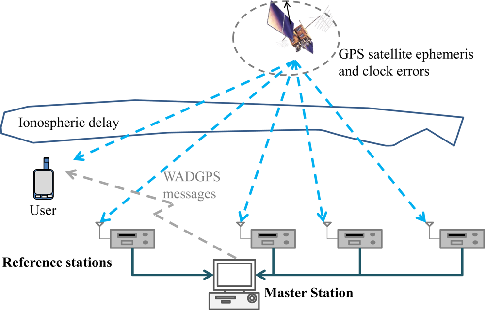
3. WADGPS Architecture
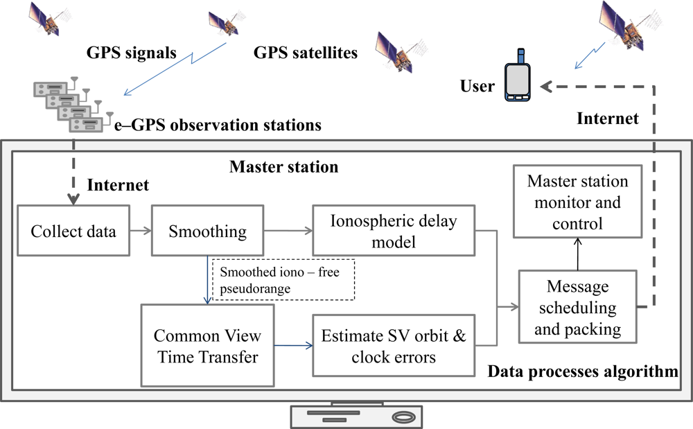
4. The WADGPS Master Station Processes
4.1. GPS Observations Modeling
- PR is the pseudorange and the subscripts L1 and L2 indicates L1 and L2 frequencies, respectively,
- is the geometric range from satellite j to user i,
- ϕ is the carrier phase and the subscripts L1 and L2 indicates L1 and L2 frequencies, respectively,
- b is the receiver clock bias,
- B is the satellite clock error,
- Nλ is the integer ambiguities and the subscripts L1 and L2 indicates L1 and L2 frequencies, respectively,
- I is the ionospheric delay at L1 frequency,
- T is the tropospheric delay,
- v is the pseudorange measurements noise and the subscripts L1 and L2 indicates L1 and L2 frequencies, respectively, and
- e is the carrier phase measurements noise and the subscripts L1 and L2 indicates L1 and L2 frequencies, respectively.
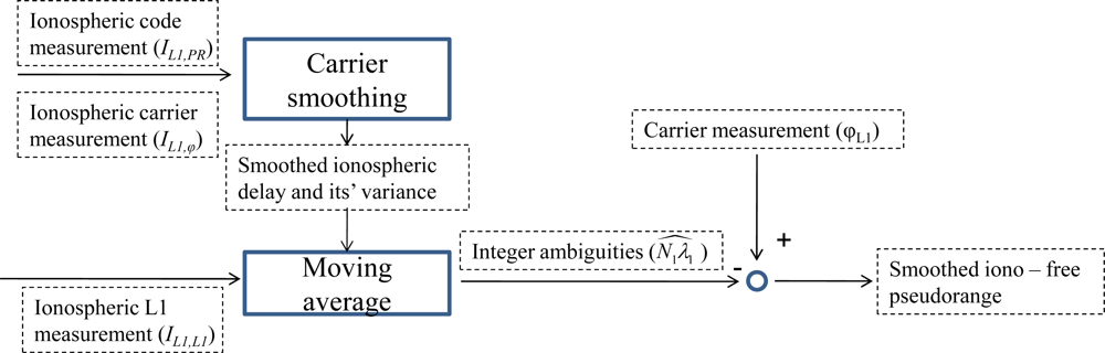
4.2. Dual-Frequency Carrier Smoothing of Pseudorange and Ionospheric Delays
- IL1 is ionospheric delay at the L1 frequency, the extra subscripts present the observations used in the combination,
- Amb is the combination of ambiguities from the L1 and L2 carrier phases, and the magnitude of noises are vPR > vL1 > vϕ[1].
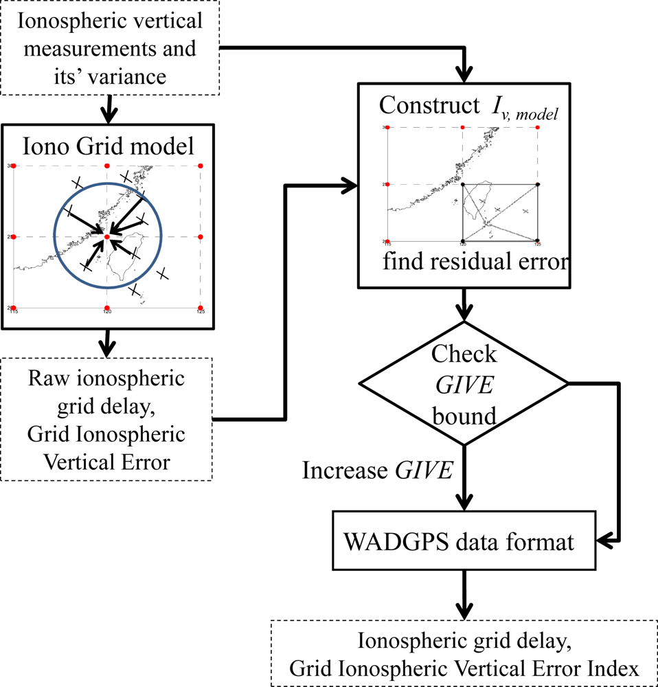
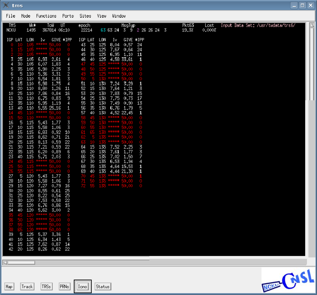
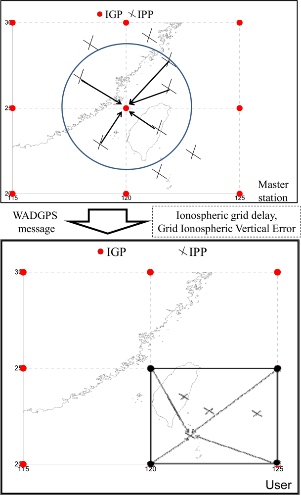
4.3. Ionospheric Corrections
- ωi is the weight of the ith IPP measurement,
- IKlobuchar,G is the vertical ionospheric delay at the grid point using the Klobuchar model parameters [1],
- IMeasure,i is the vertical ionospheric delay measurement at the pierce point, and
- IKlobuchar,i is the vertical ionospheric delay at the pierce point using the Klobuchar model parameters.
- Δ is a function of the correlation distance of the ionosphere [11].
- is the vertical ionospheric delay at the ith IPP, estimated with the broadcasted ionospheric corrections,
- IIGP,V,i is the broadcast vertical ionospheric delay at ith IGP,
- UIVEIPP,i is the user ionospheric vertical error (UIVE) which is a 99.9% confidence (error bound) on the post-correction ionospheric vertical delay residual [8], and
- GIVEi is a confidence bound of the corrected ionospheric delay residual at the ith IGP.
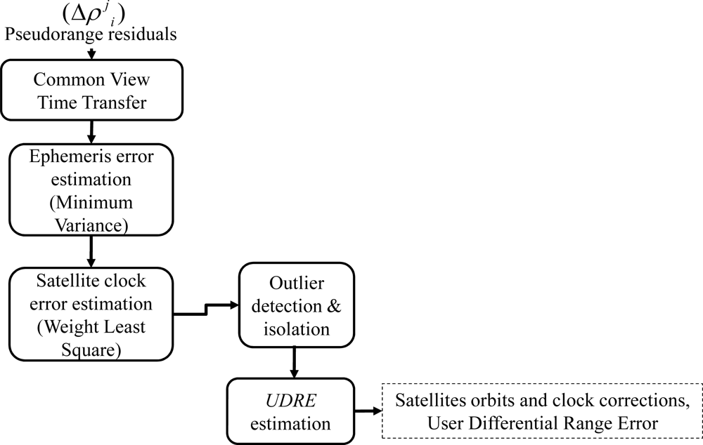
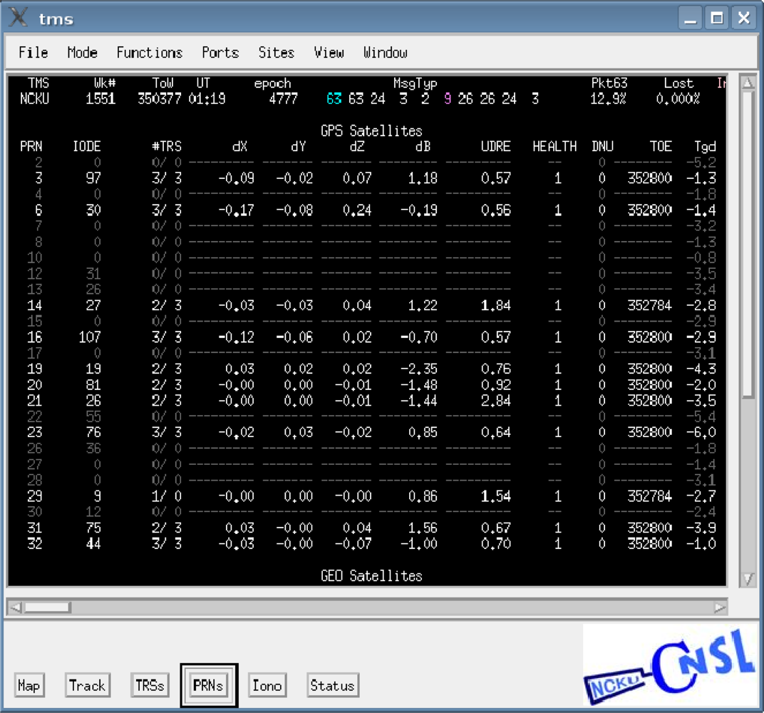
4.4. Satellite Ephemeris and Clock Corrections
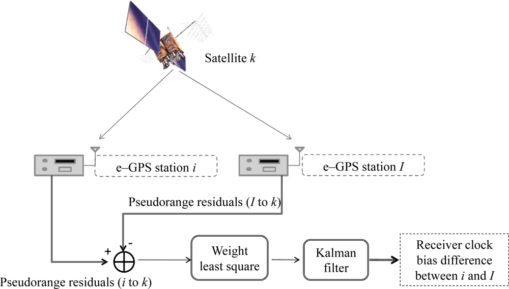
- ΔRj is the ephemeris error,
- is the unit line of sight vector from the i RS to the j satellite,
- is the unit line of sight vector from the I RS to the j satellites,
- is the line of sight difference,
- Δbi,I is the clock difference, and
- is the measurement noise.
- ΔRj is ephemeris error which is this process solving for, and
- the subscript “m” denotes the key RS which has the smallest variance [12].
- ΔRj is the ephemeris error which will be denoted as x in following discussions,
- N is number of synchronized RSs, and
- v is measurement noise with zero mean and variance of W.
- the subscript c denotes clock,
- Hc is a column vector with all 1’s,
- nc is the measurement noise with covariance matrix Wc.
- R is the measurement covariance matrix of the synchronized pseudorange residuals,
- P̂ is the covariance of the estimated ephemeris and clock errors, and
- H is the design matrix composed by unit length line of sight vectors and satellites clock term, and the line of sight vectors cover all users inside the reference network [12].
- PRi is pseudorange from the ith visible satellite,
- ΔRi is satellite ephemeris corrections,
- li is line of sight vector from the user to the satellite, and
- ΔB̂i is clock corrections.
5. Experiments and Performance Evaluation
- ■ Range data: it is composed of L1-L2 dual-frequency pseudorange, carrier phase, Doppler frequency, and signal to noise ratio of each satellite in view by the network [1]. The data update rate is 1 Hz.
- ■ Ephemeris data [15]: it includes GPS orbit parameters and satellite clock correction coefficients of each satellite in view by the network. It is updated every 50 seconds.
- ■ Almanac data [15]: it consists of the simplified GPS orbit parameters. It is updated every 500 seconds.
- ■ The Klobuchar model coefficients [15]: it provides the common ionospheric model for single frequency users. It is updated every 500 seconds
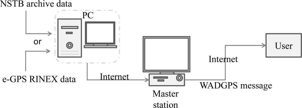
5.1. WADGPS Implementation Procedures
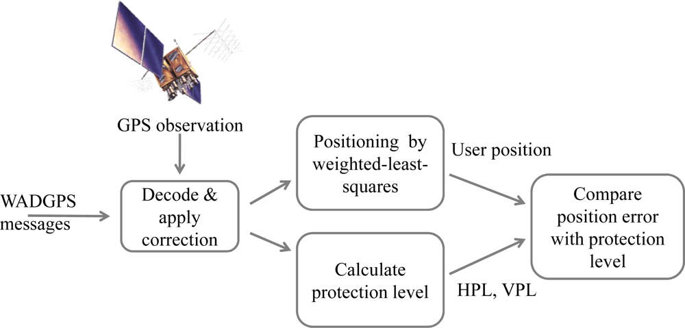
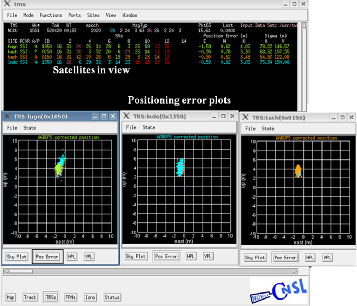
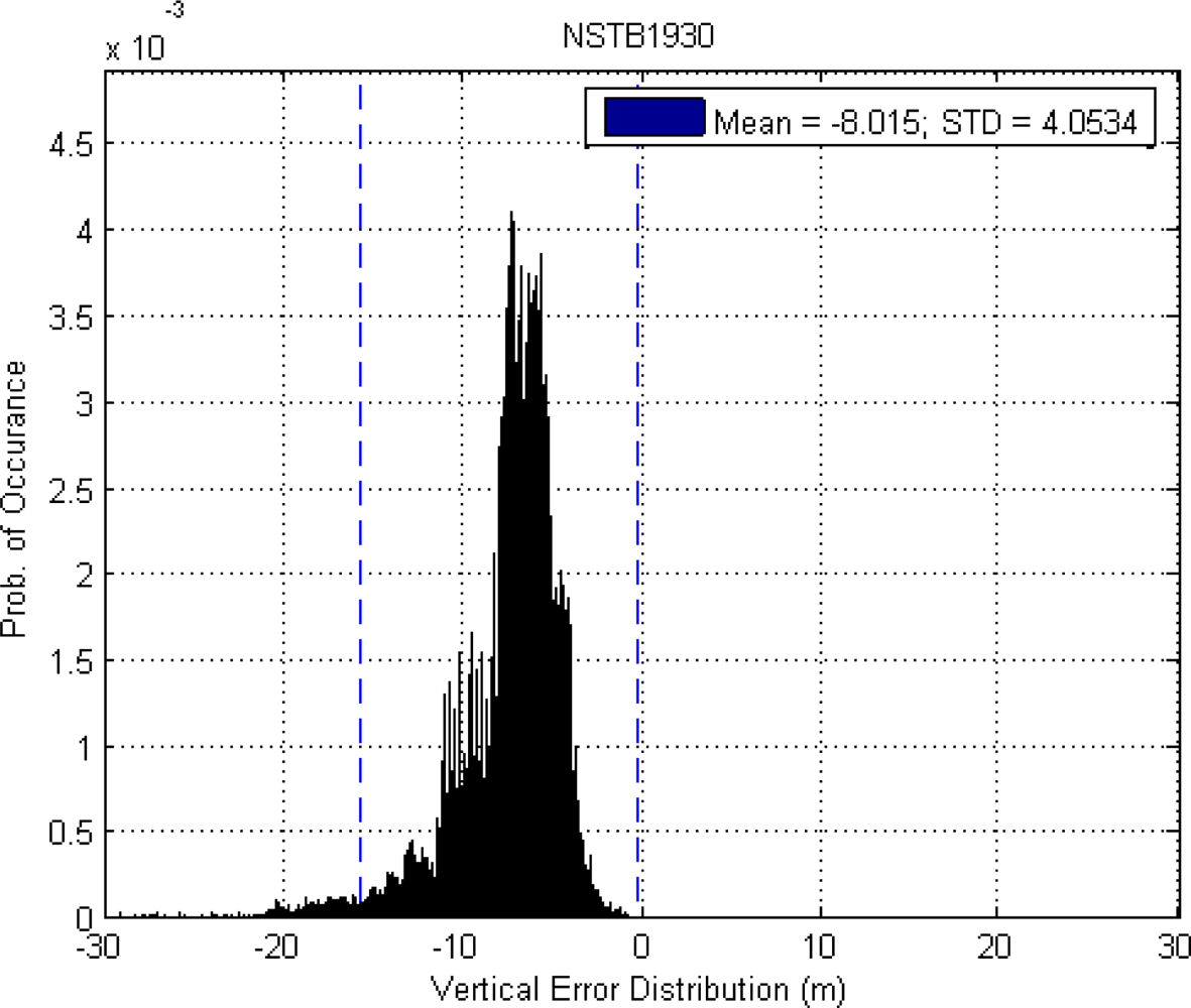
5.2. WADGPS Performance Analysis
6. Conclusions
Acknowledgments
References and Notes
- Enge, P.; Misra, P. Global Positioning System: Signals, Measurements, and Performance, 2nd ed; Ganga-Jamuna Press: Lincoln, MA, USA, 2006. [Google Scholar]
- Enge, P. Local Area Augmentation of GPS for the Precision Approach of Aircraft. Proc. IEEE 1999, 87, 111–132. [Google Scholar]
- Kee, C. Wide Area Differential GPS (WADGPS). Ph.D. Thesis, Department of Aeronautics and Astronautics, Stanford University, CA, USA, 1993.
- Enge, P.; Walter, T.; Pullen, S.; Kee, C.; Chao, Y.C.; Tsai, Y.J. Wide Area Augmentation of the Global Positioning System. Proc. IEEE 1996, 84, 1063–1088. [Google Scholar]
- Pringvanich, N.; Satirapod, C. SBAS Algorithm Performance in the Implementation of the ASIAPACIFIC GNSS Test Bed. J. Navig 2007, 60, 363–371. [Google Scholar]
- International Civil Aviation Organization (ICAO). GNSS SARPs (Standards and Recommended Practices for the Global Navigation Satellite System); ICAO: Quebec, Canada, 1999. [Google Scholar]
- Navigation and Landing Transition Strategy; Federal Aviation Administration (FAA): Washington, DC, USA, 2002.
- DO-229D. WAAS MOPS (Minimum Operational Performance Standards for Global Positioning System/ Wide Area Augmentation System Airborne Equipment); RTCA, Inc: Washington, DC, USA, 2006. [Google Scholar]
- The Stanford GPS Research Laboratory Web Site of Stanford University: Palo Alto, CA, USA. Available online: http://waas.stanford.edu (accessed on 9 February 2010).
- Kelly, R.J.; Davis, J.M. Required Navigation Performance (RNP) for Precision Approach and Landing GNSS Application. J. Navig 1994, 41, 1–30. [Google Scholar]
- Chao, Y.C. Real Time Implementation of the Wide Area Augmentation System for the Global Position System with an Emphasis on Ionospheric Modeling. Ph.D. Thesis, Department of Aeronautics and Astronautics, Stanford University, Palo Alto, CA, USA, 1997.
- Tsai, Y.J. Wide Area Differential Operation of the Global Positioning System: Ephemeris and Clock Algorithms. Ph.D. Thesis, Department of Mechanical Engineering, Stanford University, Palo Alto, CA, USA, 1999.
- Walter, T.; Enge, P.; Hansen, A. A Proposed Integrity Equation for WAAS MOPS. Proceedings of ION GPS 1997, Kansas City, MI, USA, 16–19 September, 1997.
- Jan, S.S. Aircraft Landing Using a Modernized Global Position System and the Wide Area Augmentation System. Ph.D. Thesis, Department of Aeronautics and Astronautics, Stanford University, Palo Alto, CA, USA, 2003.
- ICD-GPS-200C. NAVSTAR GPS Space Segment /Navigation User Interface; El Segundo, CA, USA, 10 October 1993. [Google Scholar]
- Chao, Y.C.; Tsai, Y.J.; Walter, T.; Kee, C.; Enge, P.; Parkinson, B.W. The Ionospheric Delay Model Improvement for the Stanford WAAS Network. Proceedings of ION NTM1995, Anaheim, CA, USA, 18–20 January, 1995.
- Kee, C.; Yun, Y.; Kim, D. Simulation-based Performance Analysis of SBAS in Korea: Accuracy & Availability. Proceedings of ION GPS/GNSS 2003, Portland, OR, USA, 9–12 September, 2003.
- FreeBSD. Available online: http://www.tw.freebsd.org/ (accessed on 9 February 2010).
- Open Motif. Available online: http://www.opengroup.org/motif/ (accessed on 9 February 2010).


| Phase of Flight | Accuracy (95% error) | Integrity | Alert Limit (H: Horizontal V: Vertical) | Continuity | Availability | |
|---|---|---|---|---|---|---|
| Time to Alarm | Pr(HMI) | |||||
| En route (continental) | H: 740 m V: NA | 15 s | 1 × 10⁻⁷ /h | H: 3,704 m V: NA | 1 × 10⁻⁵/hr | 0.99 to 0.99999 |
| Terminal | H: 220 m V: NA | 15 s | 1 × 10⁻⁷ /h | H: 1,852 m V: NA | 1 × 10⁻⁵/h | 0.99 to 0.99999 |
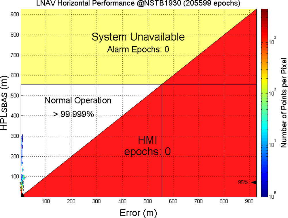
| LNAV(NPA) | H: 220 m V: NA | 10 s | 1 × 10⁻⁷ /h | H: 556 m V: NA | 1 × 10⁻⁵/h | 0.99 to 0.99999 |
| LNAV/VNAV | H: 220 m V: 20 m | 10 s | 2 × 10⁻⁷ /approach | H: 556 m V: 50 m | 5.5 × 10⁻⁵ /approach | 0.99 to 0.999 |
| LPV | H: 16 m V: 20 m | 6 s | 2 × 10⁻⁷ /approach | H: 40 m V: 50 m | 5.5 × 10⁻⁵ /approach | 0.99 to 0.99999 |
| Mean | Stand alone GPS | WADGPS |
|---|---|---|
| East (m) | −0.506 | 0.090 |
| North (m) | 0.436 | −0.085 |
| Vertical (m) | 15.707 | −7.968 |
| 95% error bound (two-sigma) | Stand alone GPS | WADGPS |
|---|---|---|
| Horizontal (m) | 7.10 | 3.55 |
| Vertical (m) | 16.10 | 8.10 |
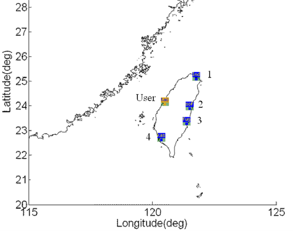
| Station No. | Station name | Latitude | Longitude |
|---|---|---|---|
| 1 | Longdong | 25° 5′50″N | 121° 55′5″E |
| 2 | Shoufeng | 23° 52′12″N | 121° 36′53″E |
| 3 | Fugang | 22° 47′26″N | 121° 12′32″E |
| 4 | Kaohsiung | 22° 37′52″N | 120° 17′18″E |
| User | Taichung | 24° 17′27″N | 120° 32′6″E |
| Mean error | Stand alone GPS | WADGPS with 3 RSs | WADGPS with 4 RSs |
|---|---|---|---|
| East (m) | 0.182 | 0.220 | 0.169 |
| North (m) | 1.785 | 1.362 | 1.498 |
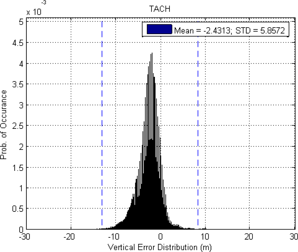
| Up (m) | 13.400 | −2.431 | −2.440 |
| 95% error bound (two-sigma) | Stand alone GPS | WADGPS with 3 RSs | WADGPS with 4 RSs |
|---|---|---|---|
| Horizontal (m) | 10.970 | 5.587 | 4.0893 |
| Vertical (m) | 19.360 | 11.248 | 11.485 |
© 2010 by the authors; licensee Molecular Diversity Preservation International, Basel, Switzerland. This article is an open-access article distributed under the terms and conditions of the Creative Commons Attribution license ( http://creativecommons.org/licenses/by/3.0/).
Share and Cite
Jan, S.-S.; Lu, S.-C. Implementation and Evaluation of the WADGPS System in the Taipei Flight Information Region. Sensors 2010, 10, 2995-3022. https://doi.org/10.3390/s100402995
Jan S-S, Lu S-C. Implementation and Evaluation of the WADGPS System in the Taipei Flight Information Region. Sensors. 2010; 10(4):2995-3022. https://doi.org/10.3390/s100402995
Chicago/Turabian StyleJan, Shau-Shiun, and Shih-Chieh Lu. 2010. "Implementation and Evaluation of the WADGPS System in the Taipei Flight Information Region" Sensors 10, no. 4: 2995-3022. https://doi.org/10.3390/s100402995