Distributed Power Allocation for Sink-Centric Clusters in Multiple Sink Wireless Sensor Networks

Abstract
:1. Introduction
- It provides a distributed transmission power control algorithm for sink nodes in multiple sink WSNs.
- By using our algorithm, less sensor nodes needs to decide which sink should act as center of local subnetworks.
- The algorithm provides a high network connectivity.
- It is targeted at multiple sink cluster-based wireless sensor networks and is the first protocol developed for these networks, to our knowledge.
A. Reachability
B. Power efficiency
C. Clustering interference
2. Related Work
- They are more reliable due to the fact that invalidation of a sink node will drag down the whole network in single sink WSNs.
- Usually there exists a serious node energy bottleneck (around sinks) if a single sink collects reports from too many sensors.
- They relieve the unbalanced energy consumption among sensor networks.
- They avoid mobile sink schemes that result in large energy consumption and serious communication interference [11].
- Multiple sinka reduce payoff of data fusion in very large and complex WSN applications [17].
- They offer more versatile functional applications and communication cooperation. In some applications, different users (sinks) may require different environmental variables (temperature, humidity, light intensity, etc.) or data formats (image, sound, video, etc.). In this time, all nodes need to cooperate with each other during the communication process.
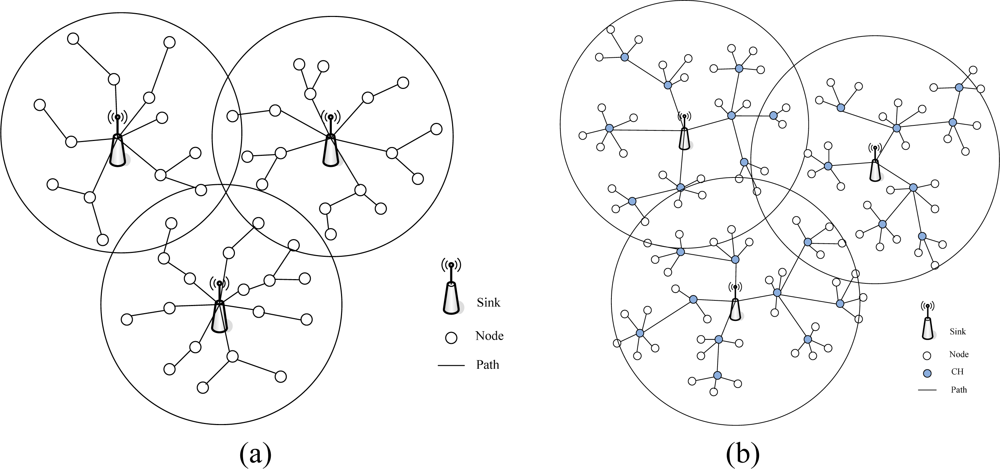
- In some cluster routing protocols, such as LEACH [5] or PEGASIS [7], each cluster head node needs to communicate with a sink node directly. If only one sink node was deployed, cluster head nodes must work with high transmission power, which not only consumes too much node energy, but also the interference problem of the long distance transmission cannot be ignored.
- They provide more real-time data transport of networks, which has a significant effect in multimedia WSNs [20].
3. System Model
3.1. Transmission Power Control Algorithms
3.2. Coverage Rate Analysis
4. Power Control For Multiple Sink Cluster WSNs (MSCWSNs-PC)
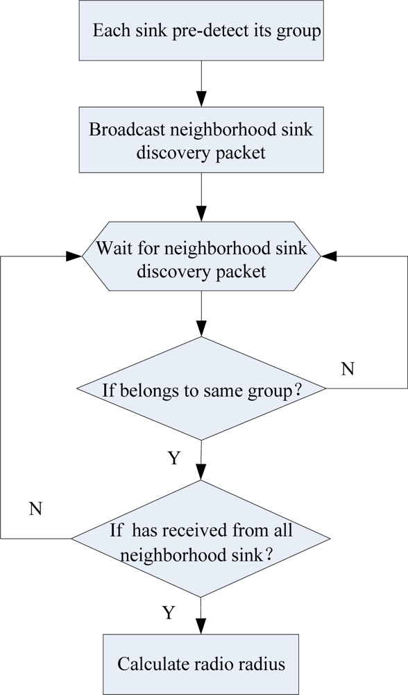
4.1. Neighborhood Sink Discovery
4.2. Distributed Power Allocation

| 01: | for all xw, w ∈ M |
| 02: | if xw>Y/2 then |
| 03: | w ∈ Topside |
| 04: | nunsinkTopside =nunsinkTopside+1 |
| 05: | XTopside(nunsinkTopside)= xw |
| 06: | YTopside(nunsinkTopsiede)= yw |
| 07: | else |
| 08: | w ∈ Underside |
| 09: | nunsinkUnderside =nunsinkUnderside+1 |
| 10: | XUnderside(nunsinkUnderside)= xw |
| 11: | YUnderside(nunsinkUnderside)= yw |
| 12: | endif |
| 13: | // |
| 14: | if xw<X/2 then |
| 15: | w ∈ Leftside |
| 16: | nunsinkLeftside = nunsinkLeftside +1 |
| 17: | XLeftside(nunsinkLeftside)= xw |
| 18: | YLeftside(nunsinkLeftside)= yw |
| 19: | else |
| 20: | w ∈ Rightside |
| 21: | NunsinkRightside = NunsinkRightside +1 |
| 22: | XRightside(NunsinkRightside)= xw |
| 23: | YRightside(NunsinkRightside)= yw |
| 24: | endif |
| 25: | endfor |
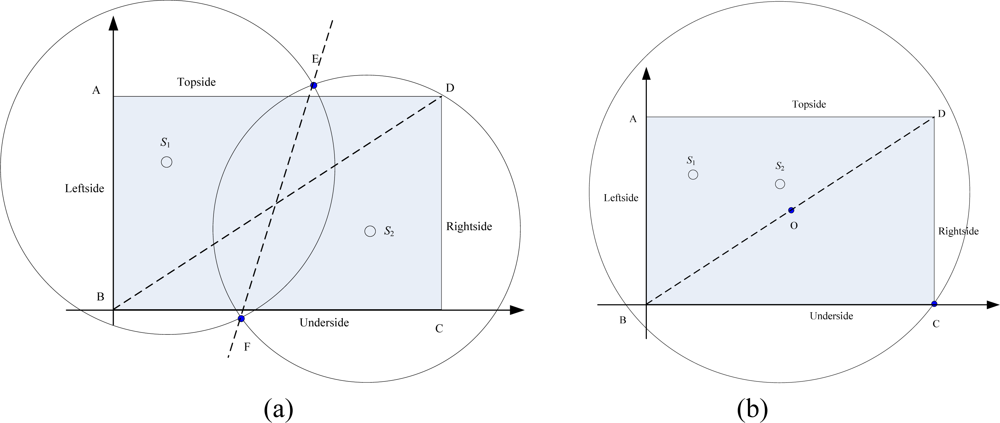
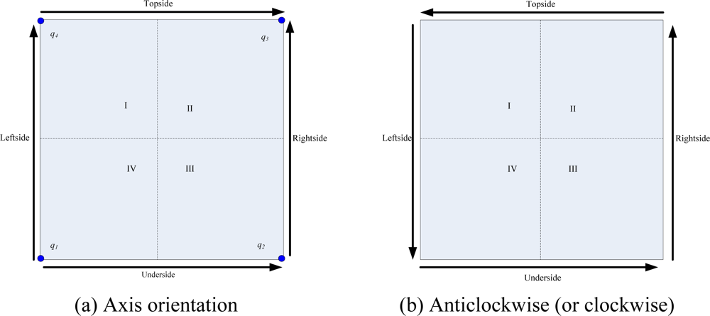
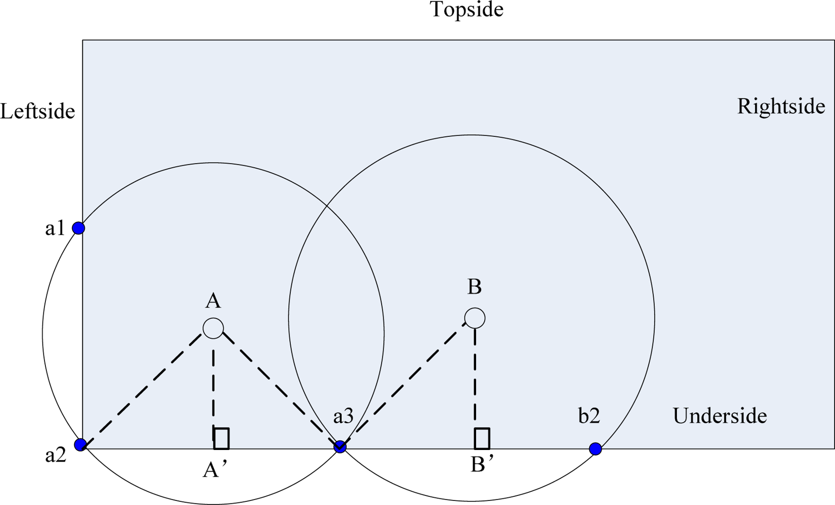
4.3. Sink Ordering Orientation
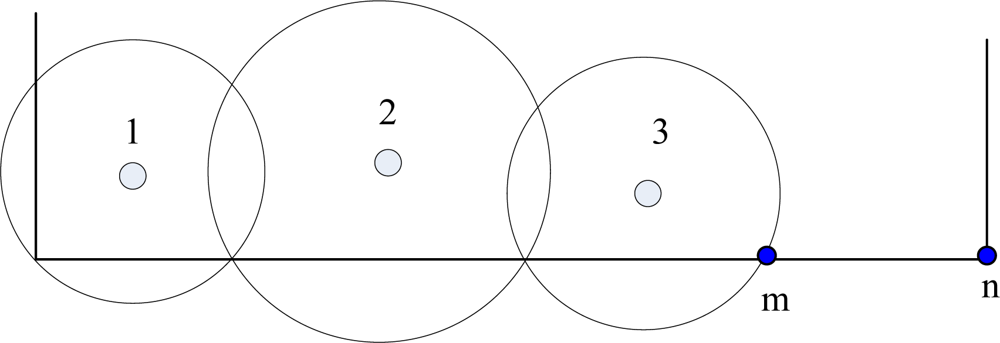
4.4. Most significant bit sink radius correction (MSBSRC)
| 01: | for all w , |
| 02: | // w∈ { max{(XTopside,YTopside)}, max{(XUnderside,YUnderside)}, |
| 03: | // max{(XLeftside,YLeftside)}, max{(XRightside,YRightside)} } |
| 04: | if Ri,j >= distance (Si, verti) then |
| 05: | // i ∈ {Topside, Underside, Leftside, Rightside} |
| 06: | // j ∈ {numsinkTopside, numsinkUnderside, numsinkLeftside, numsinkRightside} |
| 07: | Rw= Ri,j |
| 08: | else |
| 09: | Rw= distance (Si, verti) |
| 10: | endif |
| 11: | endfor |
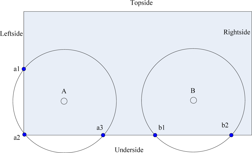
4.5. Border Constraint Problem (BCP)
| 01: | // (a) sink border group absence |
| 02: | if i==∅ then |
| 03: | for all w, w ∈ Si |
| 04: | // i ∈ {Topside, Underside, Leftside, Rightside} |
| 05: | find out the sink j which nearest to the corresponding vertex k then |
| 06: | if rj<distance(j,k) then |
| 07: | rj=distance(j,k) |
| 08: | endif |
| 09: | endfor |
| 10: | endif |
| 11: | // (b) center void |
| 12: | for all w, w ∈ Si |
| 13: | find out the sink m which nearest to the center vertex O then |
| 14: | // m ∈ {Topside, Underside, Leftside, Rightside} |
| 15: | if rm<distance(m,O) then |
| 16: | rm=distance(m,O) |
| 17: | Endif |
| 18: | endfor |
4.6. MSCWSNs-PC Algorithm Implementation
4.7. Created Clusters Communication with Sink Nodes
4.8. Mobility and Transmission Power Maintenance
5. Evaluation
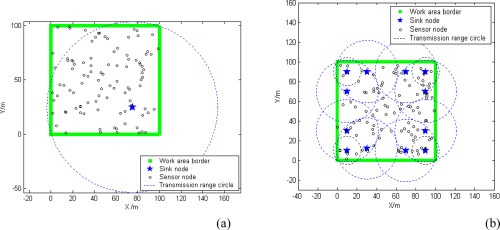
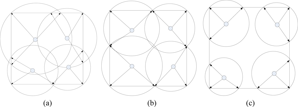
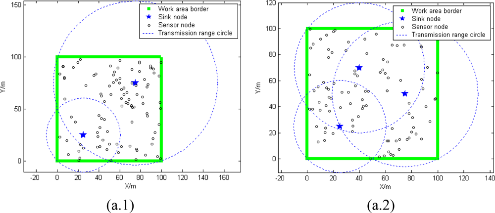
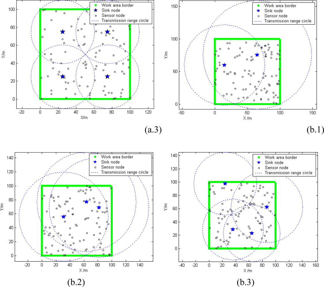
5.1. Deployment Modes of Sink Nodes
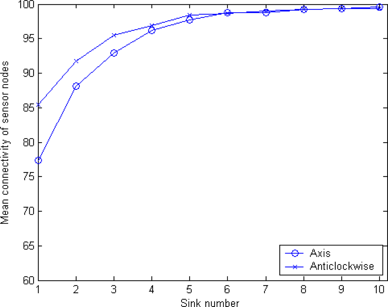
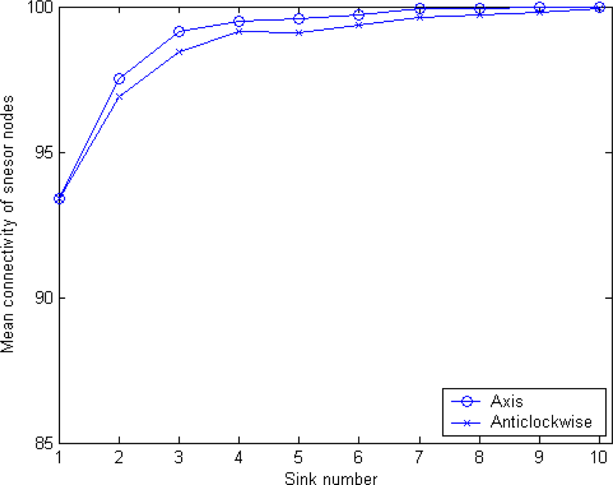
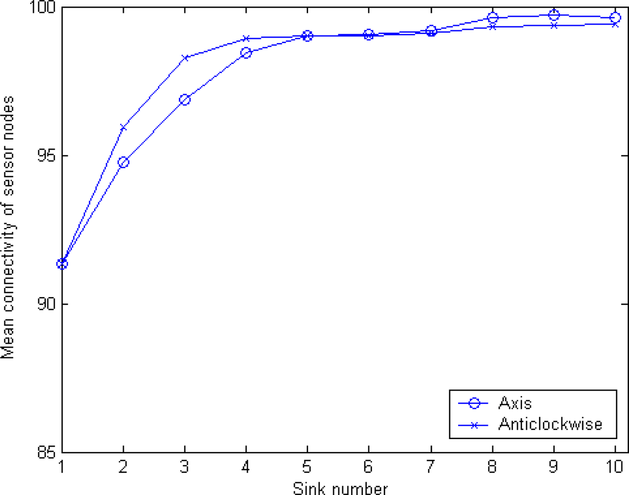
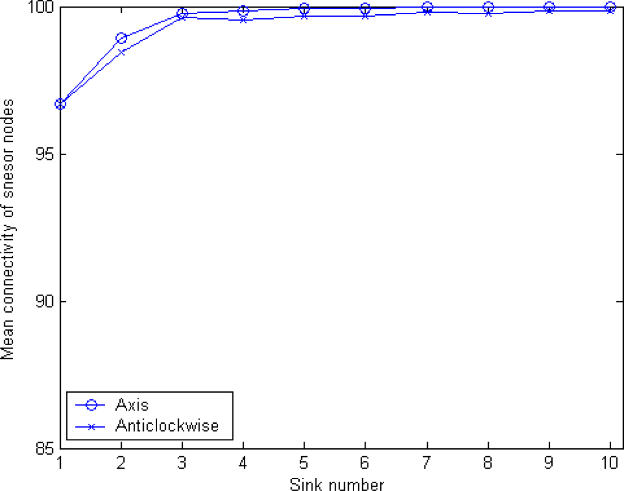
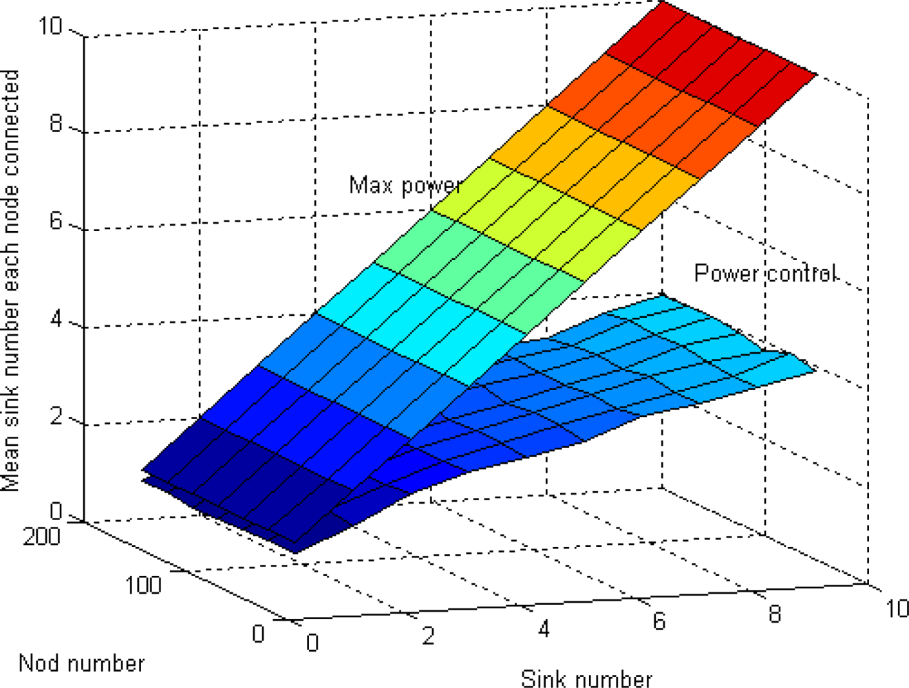
5.2. Sink Orientation to Calculate Radius and Mean Connectivity
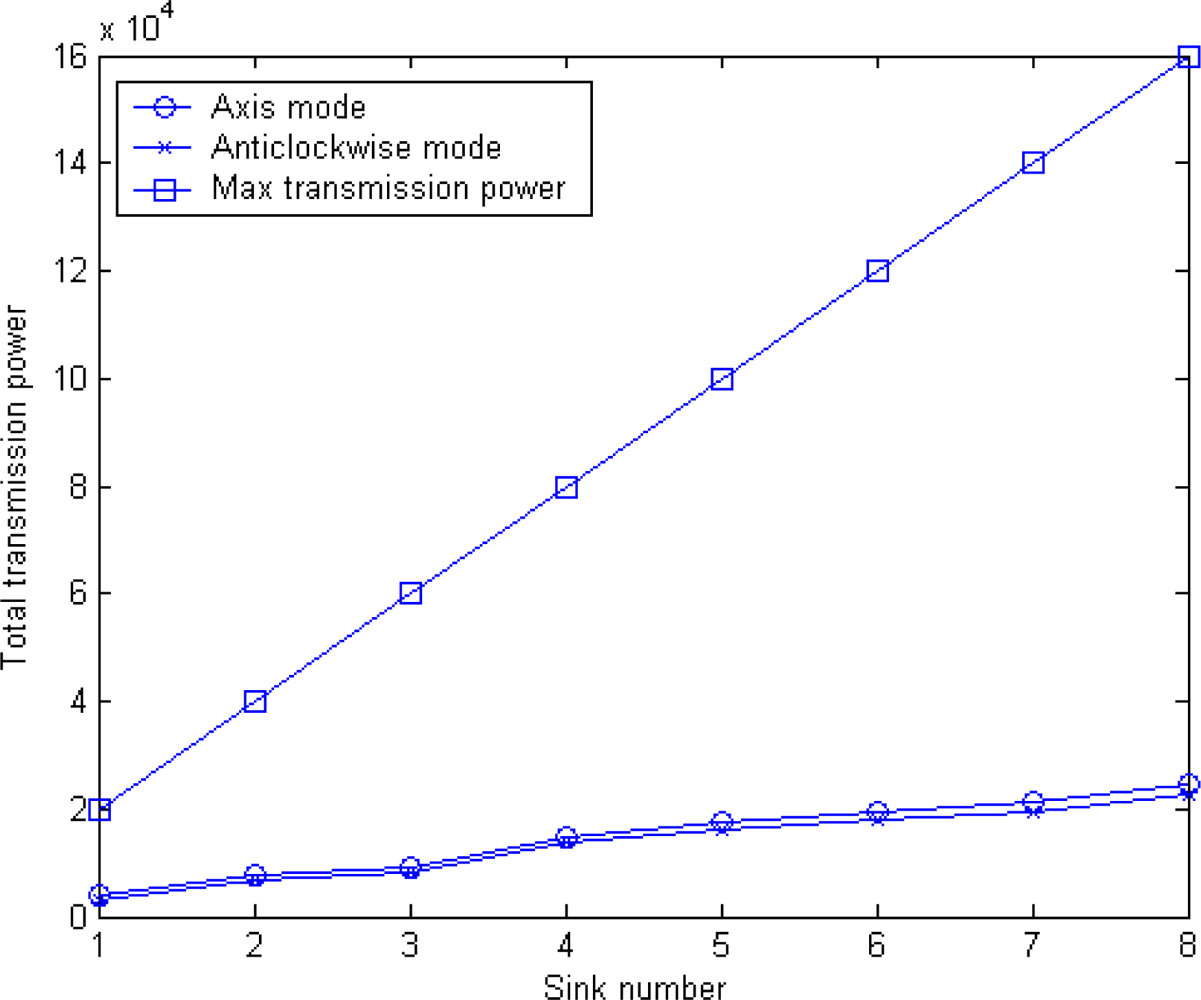
5.3. Power Efficiency
5.4. Clustering Interference
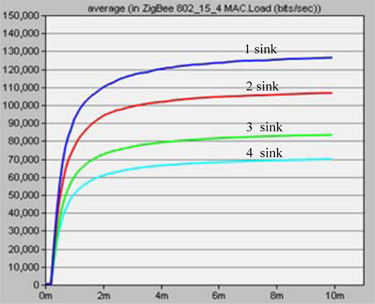
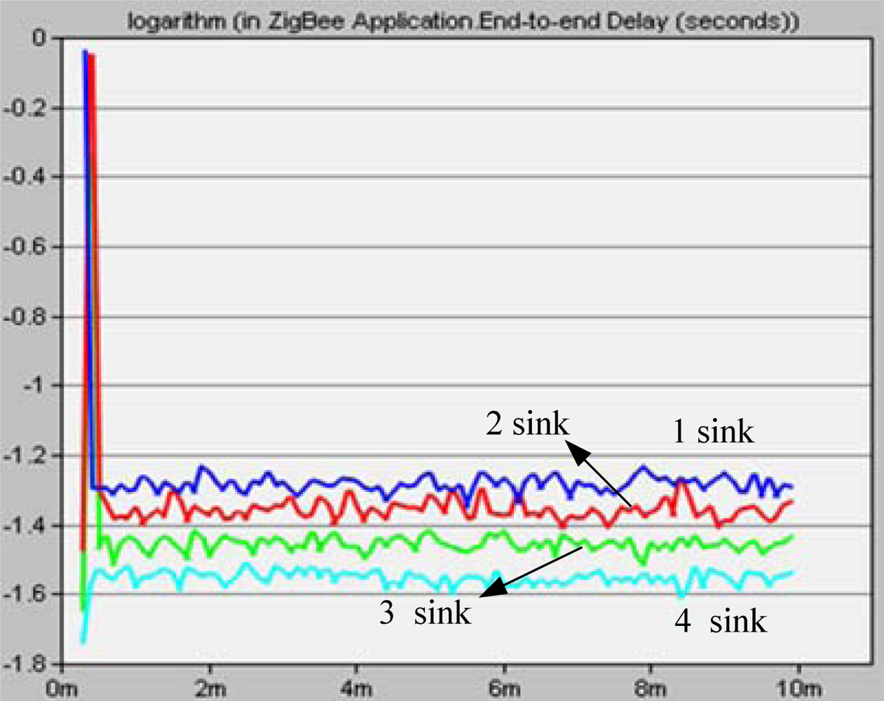
5.5. Networks Performance
6. Conclusions
References and Notes
- Clare, L.P.; Pottie, G.J.; Agre, J.R. Self-Organizing Distributed Sensor Networks. Proceedings of UGSTA, Orlando, FL, USA, April, 1999; pp. 229–237.
- Estrin, D.; Govindan, R.; Heidemann, J.; Kumar, S. Next Century Challenges: Scalable Coordination in Sensor Networks. Proceedings of MOBICOM, Seattle, WA, USA, August 1999; pp. 263–270.
- Tapas, K.; David, M.M.; Nathan, S.N.; Christine, D.P.; Ruth, S.; Angela, Y.W. An Efficient k-Means Clustering Algorithm: Analysis and Implementation. IEEE Trans.Pattern Anal. Mach. Intel 2002, 24, 881–892. [Google Scholar]
- Kohonen, T. Self-organizing maps of symbol strings; Report A42,; Helsinki University of Technology, Laboratory of Computer and Information Science: Espoo, Finland, 1996. [Google Scholar]
- Wendi, B.H.; Anantha, P.C.; Hari, B. An Application-Specific Protocol Architecture for Wireless Microsensor Networks. IEEE Trans. Wirel. Commun 2002, 1, 660–670. [Google Scholar]
- Manjeshwar, A.; Agrawal, D.P. TEEN: a routing protocol for enhanced efficiency in wireless sensor networks. Proceedings of IPDPS, San Francisco, CA, USA, April 2001; pp. 2009–2015.
- Stephanie, L.; Cauligi, S.R. PEGASIS: Power-Efficient Gathering in Sensor Information Systems. Proceedings of the IEEE Aerospace Conference, Big Sky, MO, USA, March 2002; pp. 1125–1130.
- Kim, H.; Seok, Y.; Choi, N.; Choi, Y.; Kwon, T. Optimal Multi-sink Positioning and Energy-efficient Routing in Wireless Sensor Networks. Lect. Notes Comput. Sci 2005, 3391, 264–274. [Google Scholar]
- Oyman, E.I.; Ersoy, C. Multiple Sink Network Design Problem in Large Scale Wireless Sensor Networks. Proceedings of ICC, New York, NY, USA, June 2004; pp. 3663–3667.
- Oyman, E.I. Multiple Sink Location Problem and Energy Efficiency in Large Scale Wireless Sensor Networks, Ph.D. Thesis,; Bogazici University: Istanbul, Turkey, 2004.
- Ye, F.; Luo, H.; Cheng, J.; Lu, S.; Zhang, L. A two-tier data dissemination model for large-scale wireless sensor networks. Proceedings of MOBICOM, Atlanta, GA, USA, September 2002; pp. 148–159.
- Meng, M.; Wu, X. L.; Jeong, B.S.; Lee, S.; Lee, Y.K. Energy Efficient Routing in Multiple Sink Sensor Networks. Proceedings of ICCSA, Kuala Lumpur, Malaysia, August 2007; pp. 561–566.
- Liu, H.; Zhang, Z. L.; Srivastava, J.; Firoiu, V. PWave: A multi-source multi-sink anycast routing framework for wireless sensor networks. Lect. Notes Comput. Sci 2007, 4479, 179–190. [Google Scholar]
- Frank, Y.; Sung, L.; Wen, Y. F. Multi-sink Data Aggregation Routing and Scheduling with Dynamic Radii in WSNs. IEEE Commun. Lett 2006, 10, 692–694. [Google Scholar]
- Taddia, C.; Mazzini, G. Performance of multisink geographic routing with different distance metrics. Proceedings of SoftCOM, Split-Dubrovnik, Croatia, September 2007; pp. 1–5.
- Nathalie, M.; David, S.R.; Ivan, S. Guaranteed delivery for geographical anycasting in wireless multi-sink sensor and sensor-actor networks. Proceedings of INFOCOM, Rio de Janeiro, Brazil, April 2009.
- Tan, H.P.; Gabor, A.; Winston, K.S.; Pius, W.L. Performance Analysis of Data Delivery Schemes for a Multi-sink Wireless Sensor Network. Proceedings of AINA2008, GinoWan, Okinawa, Japan, March 2008; pp. 418–425.
- Jain, R.; Puri, A.; Sengupta, R. Geographical routing using partial information for wireless Ad Hoc networks. IEEE Personal Commun 2001, 8, 48–57. [Google Scholar]
- Karp, B.; Kung, H.T. GPSR: greedy perimeter stateless routing for wireless networks. Proceedings of Mobicom, Boston, MA, USA, July 2000; pp. 243–254.
- Akyildiz, I.F.; Melodia, T.; Chowdury, K.R. Wireless multimedia sensor networks: A survey. Wirel.Commun 2007, 14, 32–39. [Google Scholar]
- Available online: http://www.chinanews.com.cn/gn/news/2008/01-24/1144158.shtml (accessed on February 8, 2008).
- Cui, J.H. Building Autonomous Underwater Sensor Networks. Under Water Sensor Network (UWSN) Lab. Available online: http://uwsn.engr.uconn.edu. (accessed on February 8, 2008).
- Awerbuch, B.; Brinkmann, A.; Scheideler, C. Anycasting and Multicasting in Adversarial Systems: Routing and Admission Control. Technical Report,; Johns Hopkins University: Baltimore, MD, USA, 2002. [Google Scholar]
- Heinzelman, W.; Chandrakasan, A.; Balakrishnan, H. Energy-Efficient Communication Protocol for Wireless Microsensor Networks. Proceedings of HICSS, Maui, HI, USA, January 2000; pp. 4–7.
- Wesel, E.K. Wireless Multimedia communications: Networking video, voice, and Data; Addison-Wesley: Reading, MA, USA, 1998. [Google Scholar]
- Henri, D.F.; Deborah, E. Efficient and practical query scoping in sensor networks; Technical Report 39,; CENS, UCLA: Los Angeles, CA, USA, April 2004. [Google Scholar]
- Hu, L. Distributed code assignments for CDMA packet radio networks. IEEE/ACM Trans. Netw 1993, 1, 668–677. [Google Scholar]
- Rappaport, T. Wireless Communications: Principles & Practice, 2nd ed; Prentice-Hall: Englewood Cliffs, NJ, USA, 1996. [Google Scholar]
- Wang, A.; Heinzelman, W.; Chandrakasan, A. Energy-scalable protocols for battery-operated microsensor networks. Proceedings of SiPS ’99, Taipei, Taiwan, China, October 1999; pp. 483–492.


© 2010 by the authors; licensee Molecular Diversity Preservation International, Basel, Switzerland. This article is an open access article distributed under the terms and conditions of the Creative Commons Attribution license (http://creativecommons.org/licenses/by/3.0/).
Share and Cite
Cao, L.; Xu, C.; Shao, W.; Zhang, G.; Zhou, H.; Sun, Q.; Guo, Y. Distributed Power Allocation for Sink-Centric Clusters in Multiple Sink Wireless Sensor Networks. Sensors 2010, 10, 2003-2026. https://doi.org/10.3390/s100302003
Cao L, Xu C, Shao W, Zhang G, Zhou H, Sun Q, Guo Y. Distributed Power Allocation for Sink-Centric Clusters in Multiple Sink Wireless Sensor Networks. Sensors. 2010; 10(3):2003-2026. https://doi.org/10.3390/s100302003
Chicago/Turabian StyleCao, Lei, Chen Xu, Wei Shao, Guoan Zhang, Hui Zhou, Qiang Sun, and Yuehua Guo. 2010. "Distributed Power Allocation for Sink-Centric Clusters in Multiple Sink Wireless Sensor Networks" Sensors 10, no. 3: 2003-2026. https://doi.org/10.3390/s100302003