1. Introduction
A pedestrian or personal navigation system provides position information about a person indoors or outdoors. For example, if a firefighter carrying a personal navigation system is injured in the line of duty, we can know her/his position from the information transmitted by a pedestrian navigation system. Pedestrian navigation systems using inertial sensors are proposed in [
1–
6]. The main advantage of inertial sensor-based systems is that they are environment-independent; pedestrian navigation systems using vision or wireless communication require that landmarks or wireless nodes be installed in the environments [
7,
8].
There are many different pedestrian navigation systems using inertial sensors. They use similar inertial navigation algorithms to compute the position [
9,
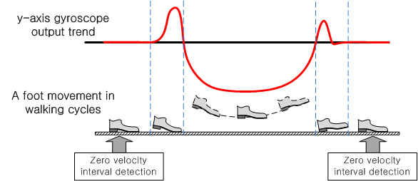
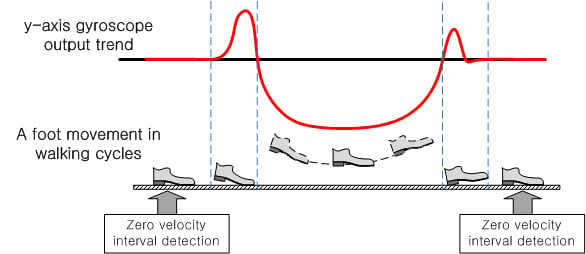
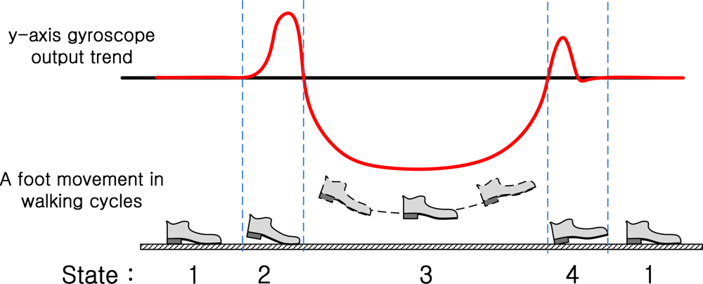
10]. Also they all use zero velocity updating algorithms. When an inertial navigation algorithm is used, the position and velocity errors diverge by a few seconds without error resetting. During normal walking cycles, a foot touches the ground almost periodically and stays on the ground for a short time (usually about 0.1∼0.3 s), which is called the zero velocity interval. In the zero velocity updating algorithm, this zero velocity interval is detected and thus the velocity error is reset to zero. Accordingly the position and velocity errors diverge very slowly, and consequently being able to reliably detect this zero velocity interval is an important issue.
Slightly different zero detection algorithms are used in [
1–
3,
5,
6]. In [
1], the zero velocity interval is determined based on gyroscope and accelerometer output norms. If the outputs are less than some threshold for a predetermined time, the zero velocity interval is decided. In [
2,
3], similar algorithms are used, where the main difference is which sensor values are used. In [
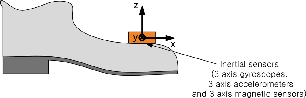
2], the zero velocity interval is determined based on
z-axis accelerometer and
y-axis gyroscope outputs (see
Figure 1 for the coordinate frame). In [
3], the zero velocity interval is determined based on norms of gyroscope outputs. In [
5], the zero velocity interval is detected based on the variance of accelerometer values. In [
6], the zero velocity interval is detected based on norms of accelerometers and gyroscopes along with variance of accelerometers.
To use the zero velocity algorithms in [
1–
3,
5,
6], some threshold values (both for sensor values and time duration) must be assigned. These threshold values could differ significantly when a person is walking and running. The sensor values tend to become large and the interval duration tend to become shorter when a person is running. If we choose the threshold values too small, then we cannot detect zero velocity intervals when a person is running. On the other hand, if the threshold values are too large, then we could detect wrong zero velocity intervals. In general, the methods in [
1–
3,
5,
6] are relatively good for walking scenarios, but not for both walking and running.
In this paper, we propose a new zero velocity detection algorithm using a hidden Markov model [
11,
12]. The most relevant result is [
4], where a zero velocity detection algorithm using a hidden Markov model is also used. The main differences are twofold. One is that only one gyroscope value is used in this paper while a foot sensor is also used in [
4], which makes the zero detection problem relatively easy. The other difference is that a Markov model is constructed using segmentation of gyroscope outputs instead of using gyroscope outputs directly, which makes the zero velocity detection more reliable.
3. Hidden Markov Model
In this section, we introduce a hidden Markov model for the zero velocity detection. The walking states are modeled as a finite state machine (see
Figure 4), whose states can be observed through
y-axis gyroscope value
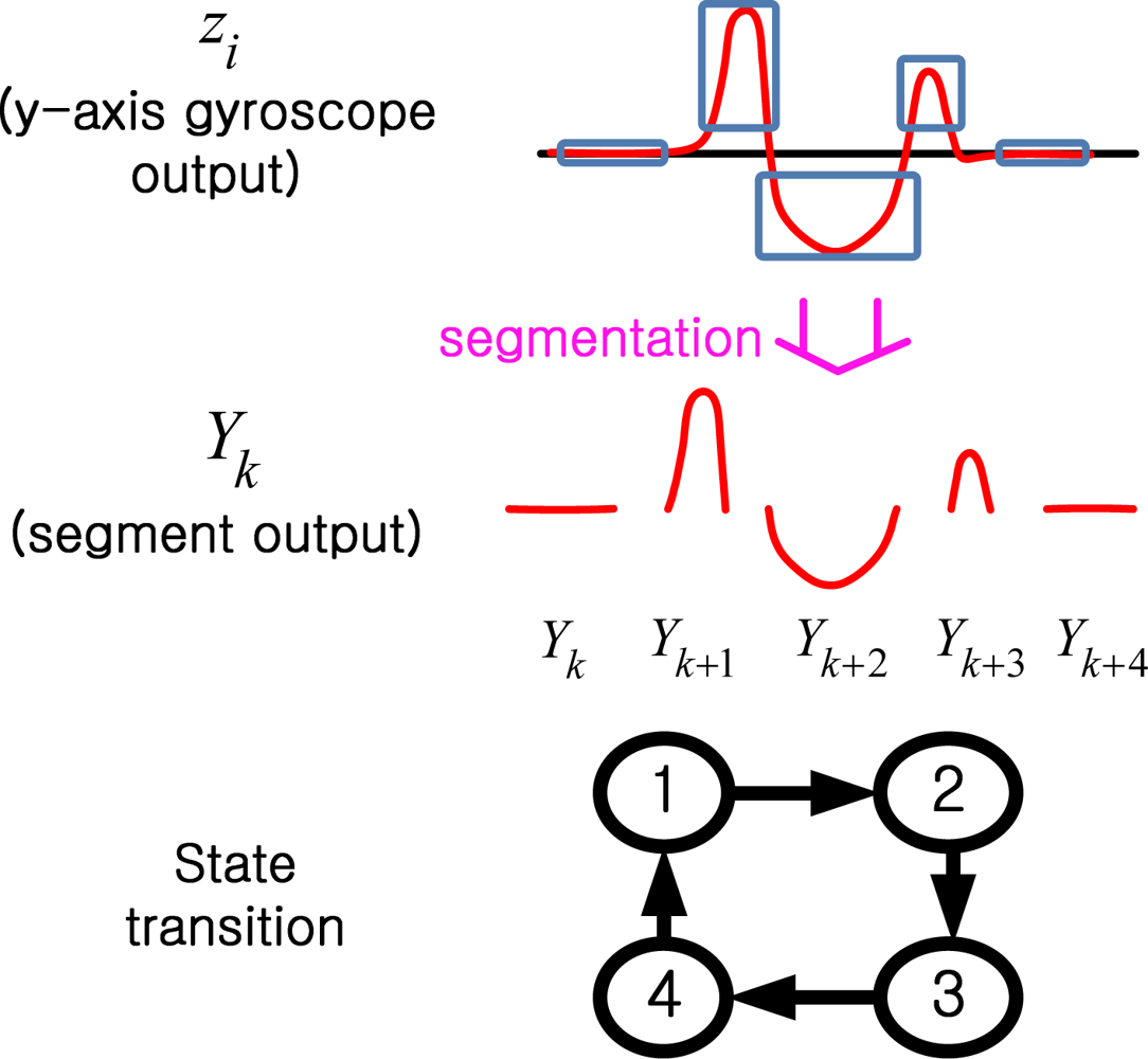
zi Instead of using
zi directly as in [
4],
Yk (a series of segments derived from
zi) is used as an output in the hidden Markov model.
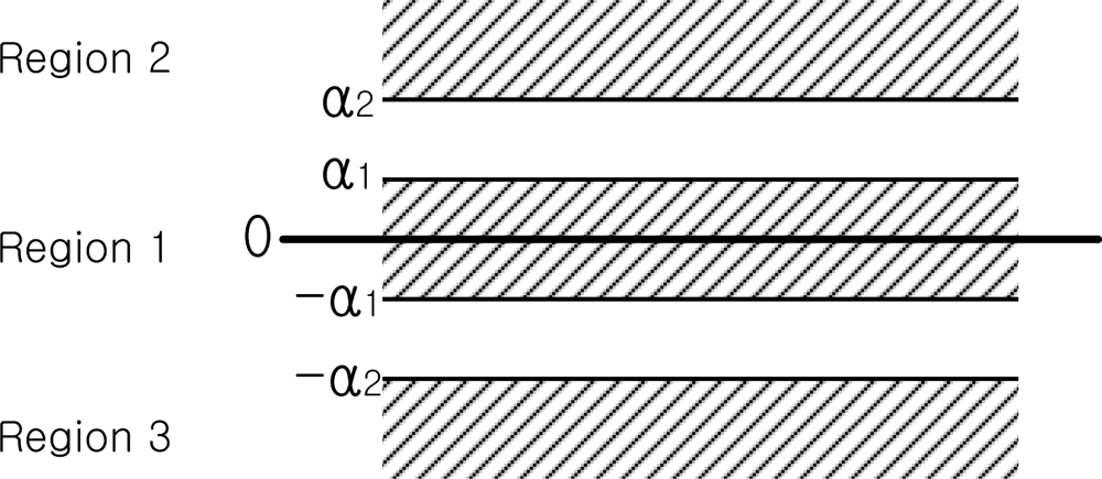
The segmentation of
y-axis gyroscope value
zi is explained. First three regions (Region 1, 2, and 3) are defined depending on
zi values (see
Figure 5). To formally state this, we define a function
f(
zi):
If zi values stay in the region j more than Nj (j = 1,2,3) (that is, at least Nj consecutive zi values have the same f(zi)), those zi values make a segment.
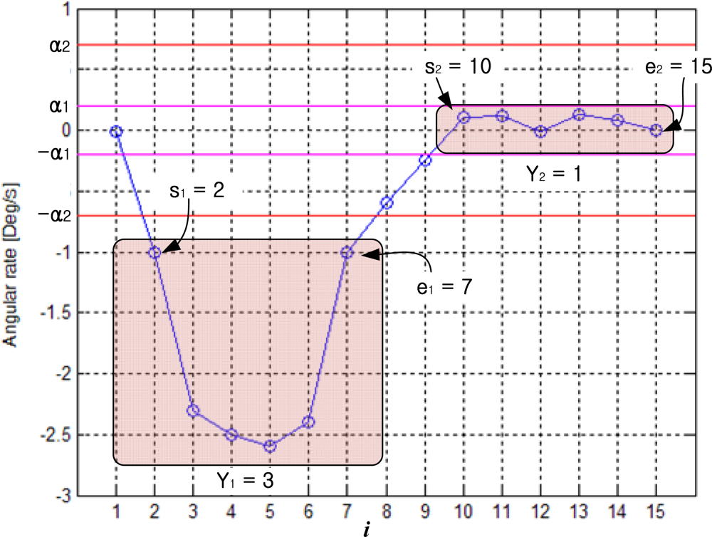
A segmentation example of is given in
Figure 6 with
N1=
N2=
N3=3. Since six consecutive
zi (2≤
i≤7) values have the same
f(
zi) =3 (that is 6≥
N3 = 3), they form the first segment. We will use
Yk (
k is the segment index) to denote the segment value, which is defined by
Yk =
f(
zi), where
zi belongs to the
k-th segment. In
Figure 6, we note that
Y1=3. Similarly, the second segment is
Y2=1. Also note that some
zi values do not belong to any segments. For example,
z8 and
z9 do not belong to any segments and these values are ignored.
In
Figure 6,
sk and
ek denote the starting and ending indices of the
k-th segment, respectively: note that
s1 = 2,
e1 = 7,
s2 =10 and
e2 =15.
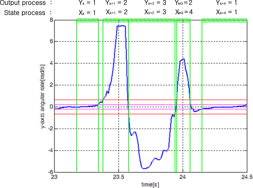
We will identify each segment using the finite state hidden Markov model. We assume that there is a Markov process
Xk, which represents four walking states in
Figure 3.
Xk assumes one of four states: 1, 2, 3, and 4. When a person is walking, a typical state transition is 1→2→3→4→1→…. The Markov process
Xk cannot be obtained directly but is estimated through the output
Yk (that is, segment output), which can be observed. An example of state transitions of
Xk and output
Yk is given in
Figure 7.
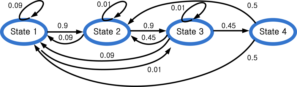
From experimental results, we determined the state transition probability as in
Figure 8. A typical state transition is 1→2→3→4→1. However, there are also other possible transition patterns. For example, 4→3→2 transition (state 1 is missing) is possible. In this case, output data corresponding to state 1 is too short to be recognized as
Yk and state 1 is considered to be missing.
From
Figure 8, the state transition probability matrix
A is given by:
where the (
m,n) -th element of
A is given by:
The determination of
A is a trial-and-error process, which is explained in the following. A normal state transition is 1→2→3→4→1→2→3→4. If walking and running cycles consist of only normal transitions,
A should be as follows:
However, we found that some states are missing during walking and running. A person walked or ran 30 steps and we examined
Yk. If no state is missing,
Yk should be 1→2→3→2 for one walking or running cycle. If
Yk is 1→2→3→1, then we know state 4 is missing. The results are summarized in
Table 1.
From
Table 1, we can draw the following conclusions:
- State 1 is sometimes missing (in particular, when a person is running)
- State 2 and 3 are not missing
- State 4 is sometimes missing (in particular, when a person is running).
Thus we modified
A1 to allow the following state transitions: 1→2→3→1 (state 4 is missing), 1→2→3→4→2 (state 1 is missing), and 1→2→3→2 (state 1 and 4 are missing):
If we choose large p1 (for example p1= 0.9 and p2= 0.1), it tends to estimate the transition 1→2→3→4 (normal cycle) as 1→2→3→2 (state 1 and 4 are missing). On the other hand, if we choose small p1 (for example, p1 = 0.1 and p2 = 0.9), it tends to estimate the transition 1→2→3→2 (state 1 and 4 are missing) as 1→2→3→4 (normal cycle). If difference between p1 and p2 is not large, the estimation results are similar.
Finally, we added small values for most transitions to allow unusual transitions. For example, when a person is standing and idly moving foot, unusual transitions (such as 2→1) could happen.
We have explained guidelines of how
A are determined. Some values (such as 0.01 and 0.09) are determined by changing values and testing the results. We note that the proposed
A is by no means an optimal
A. As far as we know there is no analytic design procedure to derive the optimal
A as stated in [
13]. It is possible that extensive tuning of the parameters could produce better results and to derive a better tuning method is one of future topics.
If the output
Yk=1, then we can assume
Xk=1 from
Figure 7. Also if
YK=2 then
Xk is either 2 or 4. If
Yk= 3, then
Xk is 3. This observation is contained in a matrix
C, which represents the link between the output process
Yk and the state process
Xk. Matrix
C is defined by:
In this paper, we use the following
C matrix:
Once
A and
C are defined, we can estimate
Xk from the output
Yk using HMM filters or smoothers [
11–
14]. Let Π
k|k+l ∈
R4×1 be a probability vector whose
i-th element is given by Pr[X
k=
i|Y1,⋯,
Yk+l]. If
l=0, then the problem becomes an HMM filter. If
l>0, the problem becomes an HMM (fixed-lag) smoother problem. It is known that an HMM smoother gives a more reliable result than an HMM filter [
11]. We found an HMM smoother with
l=1 gives a significantly much more reliable results in our case (see the experimental results in
Table 1). For example, suppose the state 4 and 1 are missing and the state transitions are given by 1→2→3→2→3 (
Xk). In the case, the outputs are given by 1→2→3→2→3(
Yk). If we use an HMM filter, the estimated first four states are likely to be 1→2→3→4 (
Xk) since it only uses the current outputs 1→2→3→2(
Yk). On the other hand, an HMM smoother gives the correct estimates using the outputs 1→2→3→2→3(
Yk). When an HMM smoother with
l=1, we can obtain an estimation result only after the current and the next outputs are available. Thus the estimation result is delayed by the combined duration of the current and next segments: typical delay is 1 second.
4. Zero Velocity Detection Algorithm
After
Xk is estimated, the next step is to determine zero velocity intervals. We decide that the time
i belongs to zero velocity intervals if |
zi|≤α
3 with anti-chattering algorithm and
i satisfies the following conditions:
The |zi|≤α3 condition is used as a safeguard to prevent false identification of the zero velocity interval.
Case 1 corresponds to the normal walking cycles, where the state transition is 3→4→1→2 (see
Figure 7). Since the zero velocity interval belongs to the state 1, the interval is chosen inside state 1. The parameters
β1 and
γ1 are used to discard time intervals near edges of the interval whose state is 1:
Since a foot is moving before and after state 1, the foot velocity cannot be zero in the edge regions. Thus we cut 10% (corresponding to 0.1) off the interval at both edges. If we choose larger values (for example, 0.2), the chance that a non-zero velocity interval is mistakenly identified as a zero velocity interval is reduced. However, we could obtain narrower zero velocity intervals, which is not desirable.
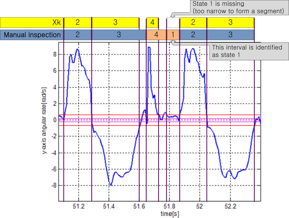
Case 2 and 3 correspond to walking or running cycles, where state 1 and/or state 4 are missing. Case 2 is when state 1 is missing. This could happen if the zero velocity interval is too short to form a segment. For example, state 1 is missing in
Figure 9: state transition is 2→3→4→2→3. However, we can identify an interval corresponding to state 1 in
Figure 9 by the manual inspection. This interval is identified as state 1 in the manual inspection. Thus the state classifications by the manual inspection and by
Xk are different: even if some states are missing in
Xk transition, they can be identified in the manual inspection.
We manually inspected the data and found the average duration ratio of each state is given as follows:
The ratio was computed from a weighted average of walking (weighting 0.1) and running (weighting 0.9) data. More weighting was given to running since missing states (like in case 2 and 3) are more likely to happen in running.
In case 2, the state 1 is missing. We assume the interval of missing state 1 is (
sk–1+
bk,sk). Note that the average duration percentage of state 4 and state 1 are 18.5% and 11.3%, respectively. Thus the duration ratio between
sk–1 and
sk is 0.621:0.379. Thus we choose
β2 and
γ2 as follows (see
Figure 10):
In other words, the interval [sk–1, sk] is divided into [sk−1,sk−1+β2] and [sk−1 +β2,sk], where the latter is considered as state 1 interval.
Case 3 is when state 4 and 1 are missing. In this case, interval [
sk–1,
sk] includes the state 3 and missing states (4 and 1). Note that the average duration percentage of state 3, 4, and state 1 are 42.8%, 18.5%, and 11.3%, respectively. Thus the duration ratio among state 3:state 4:state 1 is 0.589 : 0.255 : 0.156. Thus we choose
β3 and
γ3 as follows:
When the interval [
sk–1+
βj,
ek–1−
γj] is determined, we checked whether
zi,
i∈[
sk–1+
βj,
ek–1−
γj] satisfies |
zi|<
α3 condition. Let
U = {
i| |
zi| < α
3,
i ∈ [
sk−1 + β
j,
ek−1−γ
j]}. If the set
U consists of more than one intervals as in
Figure 11, the interval whose duration is the largest is chosen as the zero velocity interval.
5. Experiments
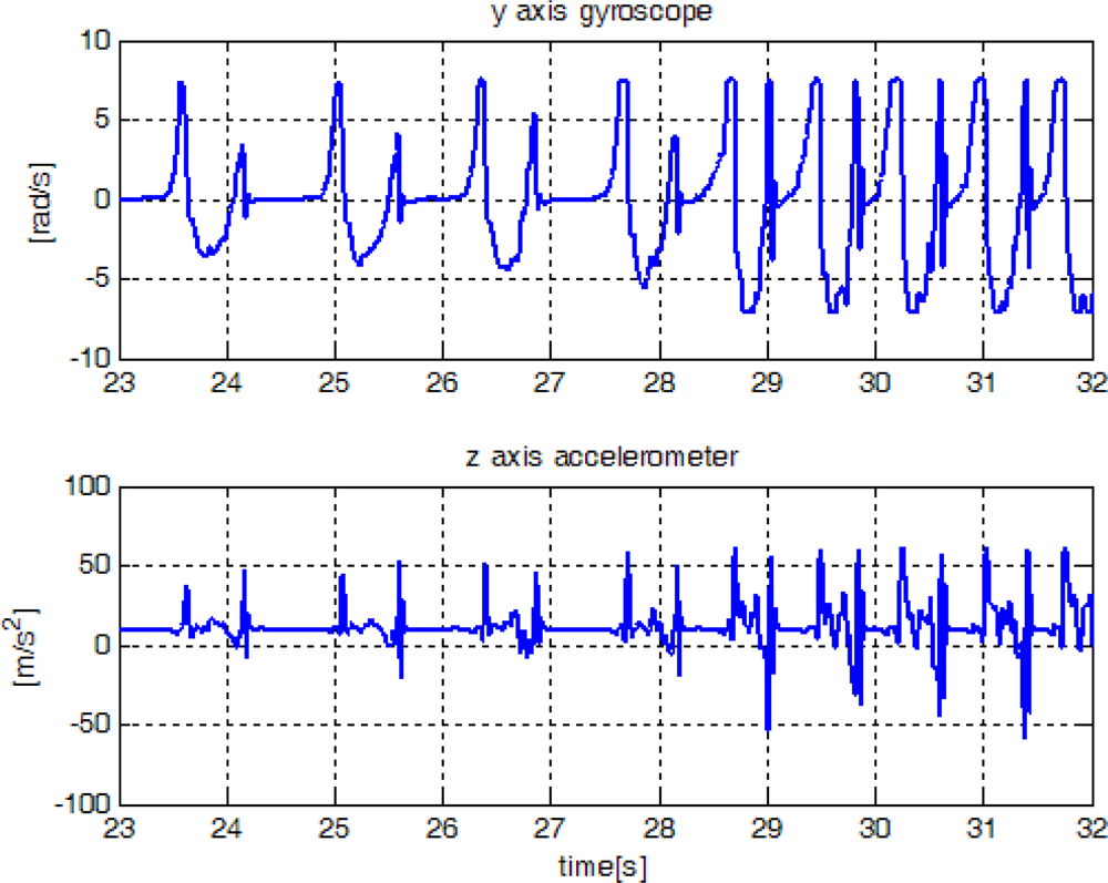
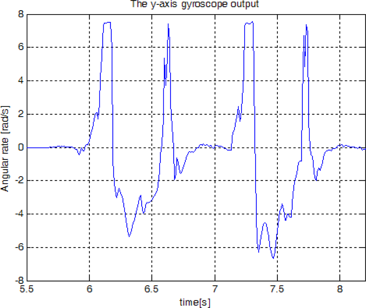
In this section, the proposed method is verified using experiment data, which are obtained from an inertial sensor unit (Xsens Mti) attached on a shoe. The sampling rate is 100 Hz. In
Figure 12, sensor outputs are given when a person walked and then ran slowly. We note that only gyroscope output is used in the proposed algorithm. The z-axis accelerometer output is also given since it is used by other existing algorithms. The proposed algorithm along with other existing algorithms [
1–
3] are applied to the experiment data. The parameters of the proposed algorithm are given by:
The parameters αj and Nj are determined from the experimental data so that normal walking gives four different states. For example, if we use a smaller α2 value, it becomes sensitive to noises so that states 2/3/4 could be falsely identified. On the other hand, if we use larger α2 value, states 2/3/4 could be lost. The parameter Nj is closely related to αj. For example, smaller N2 has a similar effect of using smaller α2 in the sense that state 2/3/4 could be falsely identified.
As a reference, zero velocity interval is determined by manually analyzing gyroscope data. When data are analyzed manually from the plot, the sensor noises and irregularities can be easily spotted and thus we can consider the detected interval as a true zero velocity interval.
The result is given in
Figure 13. The algorithm in [
1] failed to detect the zero velocity interval when a person is running. The algorithm in [
3] is not reliable in the sense that there are false zero velocity detections.
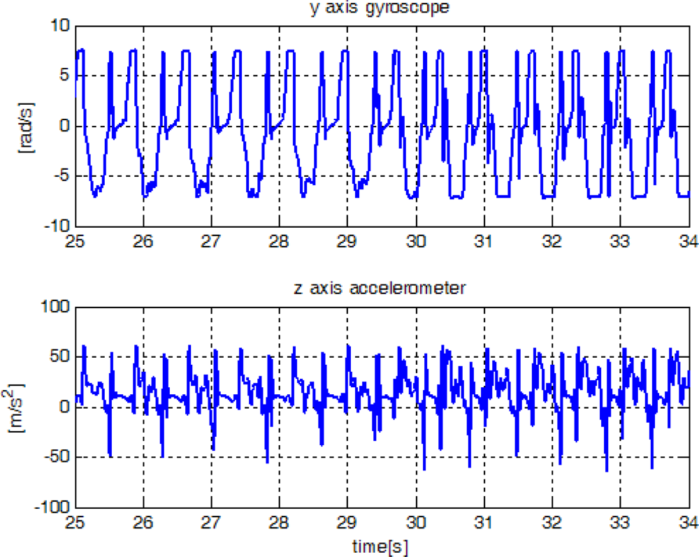
In
Figure 14, sensor outputs are given when a person ran slowly and then ran fast. The speeds of “walk”, “run slowly” and “run fast” are about 1.05 m/s, 2.14 m/s, and 3.50 m/s, respectively, which are computed by dividing the distance by the elapsed time. The zero detection results are given in
Figure 15. It can be seen that the methods in [
1] and [
2] cannot detect the zero velocity intervals when a person ran fast. In all cases (
Figures 13 and
15), the proposed algorithm reliably detected the zero velocity intervals.
To compare performance of each method quantitatively, a person walked or ran 30 steps at different speed. Since there is one zero velocity interval in each step, 30 zero velocity intervals should be detected. The number of detected zero velocity intervals by different methods is given in
Table 2. We can see when a person is walking, all methods give a good result. When a person is running, method 1 and 2 failed to detect the zero velocity intervals most times. The method [
3] and the proposed method with an HMM smoother are able to detect all the zero velocity intervals. When counting the number of detected zero velocity intervals, we counted one even if there are more than two detection during the same zero velocity interval. For example, see the two detected zero velocity intervals by the method [
3] between 24 and 25 s. These two intervals are counted as one interval. We note that there is a zero velocity interval between the two detected zero velocity intervals, but it is not detected by the method [
3]. On the other hand, the proposed method detects almost the whole range of a zero velocity interval. Thus the proposed method can detect the zero velocity intervals more reliably.
We also investigated whether there is false zero velocity detection (an interval is identified as a zero velocity interval while a foot is not in the zero velocity interval). The result is given in
Table 3, where the same experiment data were used as in
Table 2. It can be seen that the method in [
3] sometimes falsely identifies the zero velocity intervals: we found the method in [
3] sometimes falsely identifies zero crossing points of gyroscope norm as zero velocity intervals. There was no false zero velocity detection in other methods.


