1. Introduction
We start with what may seem like a trivial question: assume that you have been told that a series of fair coin flips resulted in 60% “heads”, 40% “tails”. This is the only information given, but you already have made a judgment about how many coin flips occurred, and perhaps have generated a probability distribution in your head where the highest likelihood is for 5 or 10, rather than 50 or 100, events. This is taking advantage of what we know about the probability mass function of a binomial distribution, where the observed number of “successes“ in a series is related to the probability of success (here, presumably 50%) and the number of trials. A large error from our expectations is what suggests the low sample size from that distribution.
Here, we consider whether the same principle could be used for improving the efficiency of exploring the presence, distribution, and abundance of genetic biodiversity. Documenting the distribution and abundance of biodiversity—in many habitats, at multiple scales—is critical as scientists evaluate how populations are responding to environmental change. Though technological advances have rapidly improved some elements of this [
1,
2], there are still glaring deficiencies in our ability to efficiently catalog diversity, even in small domains or limited taxonomic surveys.
The most apparent advances have been in surveys of microbial and viral diversity. Next-generation sequencing (NGS) has permitted the now-commonplace exploration of fungal, bacterial, and viral diversity by generating 10
5–10
7 sequence reads per sample and using barcoding approaches (match of sequence to known taxonomic samples for that genomic region) to identify the lineages, OTUs, or species present and their relative abundance. While there is no doubt that this has transformed our understanding of functional ecosystem processes and ecology of microbes, other prokaryotes, and microscopic eukaryotes at this scale [
3,
4,
5,
6,
7], there are definite limitations—including the difficulty of reliably matching molecular sequence data to described species or taxonomic diversity [
8,
9]. For example, some taxa (e.g. Archaea) may not be as readily amplified using the same ribosomal 16S “bacteria” primers, and variation in amplification efficiency certainly exists within the Eubacteria [
10]. Additionally, it is known that some bacterial genomes harbor more than one copy of this canonical locus [
11], thus muddling the relationship between read frequency and taxon frequency in a community.
The same problems exist—and are exacerbated—when studying multicellular diversity. On top of the problems of potential contamination, detecting rare taxa and/or handling singleton evidence for rare taxa, there is potentially a large variance in individual sizes of organisms. This, along with amplification variation given mismatches in the primer region, means that the relative read abundance in a NGS data set will often wildly vary (by multiple orders of magnitude) from the abundance of actual tissue in the data set [
3,
8,
9,
12,
13]. Researchers tend to address this by analyzing data for simple incidences as well as relative read abundance, to identify patterns robust to either removal of information or inaccurate information [
3].
If, however, the goal is to understand the actual relative abundance of individuals of different species in a sample—with these species harboring variation at “barcode” loci, and often being highly divergent from one another—our question is whether there is complementary information that can be extracted from these data that does not rely on the abundance of reads that are assigned to a taxon, but relies on our understanding of diversity within populations, how that pertains to the effective population size, and how that can be measured.
The summary statistics for DNA sequence diversity are well established and generally recognize the population mutation rate θ at a given locus; as a population increases in size (N), or as the mutation rate μ at that locus increases, more polymorphisms and more diversity will be found (θ is proportional to Nμ). There are limitations to this approach based on Kimura’s neutral theory, as various forms of genomic selection will limit the direct relationship between population size and population diversity [
14,
15,
16]. Nevertheless, these summary statistics—including Watterson’s θ, a sample-normalized estimator that uses the number of segregating sites
S in a sample—may provide information necessary to generate
some inference of relative abundance from NGS data. This information also has its limits: nucleotide diversity (π) requires information on polymorphic site frequencies that will be biased by differential amplification across individuals, as well as relatively uninformative—or diminishing—returns as the number of sampled individuals increases [
17]. Haplotype diversity (
H) is likely sufficient to set a minimum boundary on the number of individuals sampled, and
H along with
S may provide enough information to generate a probabilistic distribution associated with larger numbers of individuals.
Here we present the mathematical considerations necessary to develop estimates of the relative abundance of species in a barcoding sample of unknown number of individuals. The tools combine previous information on genetic diversity in the sampled population (that is, a species or population that has previously been analyzed at the same locus) with observed properties of the sample, such as the number of haplotypes and the number of segregating sites for each species. Our approach is distinct from the difficult problem of matching molecular OTUs with nominal taxa [
6,
18], which may require a specific database of reference taxa for the region being studied and assessment of how sensitive the results are to the criteria used for defining populations. We then evaluate the situations in which there is sufficient power to make meaningful statements about relative abundance from polymorphism data alone. It should be noted that here we are considering the dynamics only of single-copy mitochondrial haplotypes or gene regions that can generally be considered to only have a single diversity lineage within individuals and the taxon they represent.
2. Experimental Section
Our approach is to identify information that can be used as prior information to establish the likelihood of observing polymorphism data from an unknown number of input individuals (or gene copies in the case of a single-copy diploid marker) for a taxon. Any type of sampling information may help to set an upper limit: for example, if it is known that only 200 individual specimens (of all taxa) were originally used for isolation of DNA, then the maximum number of total individuals inferred from this approach should be 200 for any single included population. This itself is not a major advance in biology, but a limit on the inference nonetheless.
There are also clear minimum bounds that can be established for the abundance of a taxon. Considering DNA sequence haplotypes as our most basic sample of genetic diversity, we ask how many distinct haplotypes are recovered in the data that match a particular taxon? For a haploid mitochondrial marker (such as the oft-applied cytochrome oxidase I (COI) gene region), this number is the minimum number of individuals present (if the number happens to be zero, it is also likely to be the maximum number of individuals in the sample!). Diploid markers will be more complex to interpret; nevertheless the number of distinct alleles would be a minimum of the number of gene copies recovered, and for a single-copy locus there can only be one or two alleles per individual.
We suggest three methods that could help to estimate the number of individuals for a particular species in a metabarcoding sample: (1) an inference based on prior estimates of haplotype diversity of a particular population and the observed
number of haplotypes in a matched sample from that population; (2) an inference based on the expectations of Ewens’ [
19] sampling theory given a prior estimate of θ and the
number of haplotypes observed in the sample; and (3) an inference based on a prior estimate of θ in the field population and the observed
number of segregating sites in the sample.
To evaluate the potential usefulness of each method for recovering the abundance of input individuals, we simulated populations evolving under a Wright-Fisher neutral model. We performed the simulations with Hudson’s
ms program [
20] using the
gap [
21] package in R [
22]. We simulated 3 populations, using three different population mutation rates (θ of 2, 10, and 20). For each population we then calculated summary statistics using the
PopGenome [
23] package in R.
From the simulated populations (single simulations of 1000 alleles of arbitrary length given θ of 2, 10 and 20) we took “field samples” of different sizes (
n = 2, 4, 8, 16, 32, 64, 128), sampling without replacement. We replicate the sampling experiment 100 times for each combination of θ and
n, to be able to assess variance associated with the sampling effort. For each replicate, we calculate the number of haplotypes and the number of segregating sites, which represent our observed values in the simulated samples. From these distributions of observed values (haplotypes and segregating sites) in each combination of theta and sampling size we selected the values within the percentiles 0.25 and 0.75 to use in back calculations of the number of individuals in that sample. The distributions are presented in the
Supplementary Material (Figures S2 and S3). The sampling size, known to us from this design, is what we attempt to predict using the reversed inferences described below for each method.
All the analysis of the simulated populations was done in R [
22], with the exception of the estimation of predicted segregating sites according to Wakeley [
17] that were performed in the software Mathematica [
24] given floating-point errors in R. Detailed information and the R code used to performed simulations is presented in the
Appendix A1 in the Supplementary Material.
2.1. Haplotype Diversity
In addition to the simple number of haplotypes observed at a barcode marker, we may also attempt to estimate the number of individuals that harbored those haplotypes. Here, we assume that there is previous information on haplotype diversity (
H) from the natural populations of the species (or distinguishable populations) that are present in the barcoding sample. The “haplotype diversity”,
H, defined by Nei and Tajima [
25] as
represents the probability that sampling a new individual will result in observation of a new haplotype. N is the number of haplotypes, and
xi is the sample frequency of the i
th haplotype.
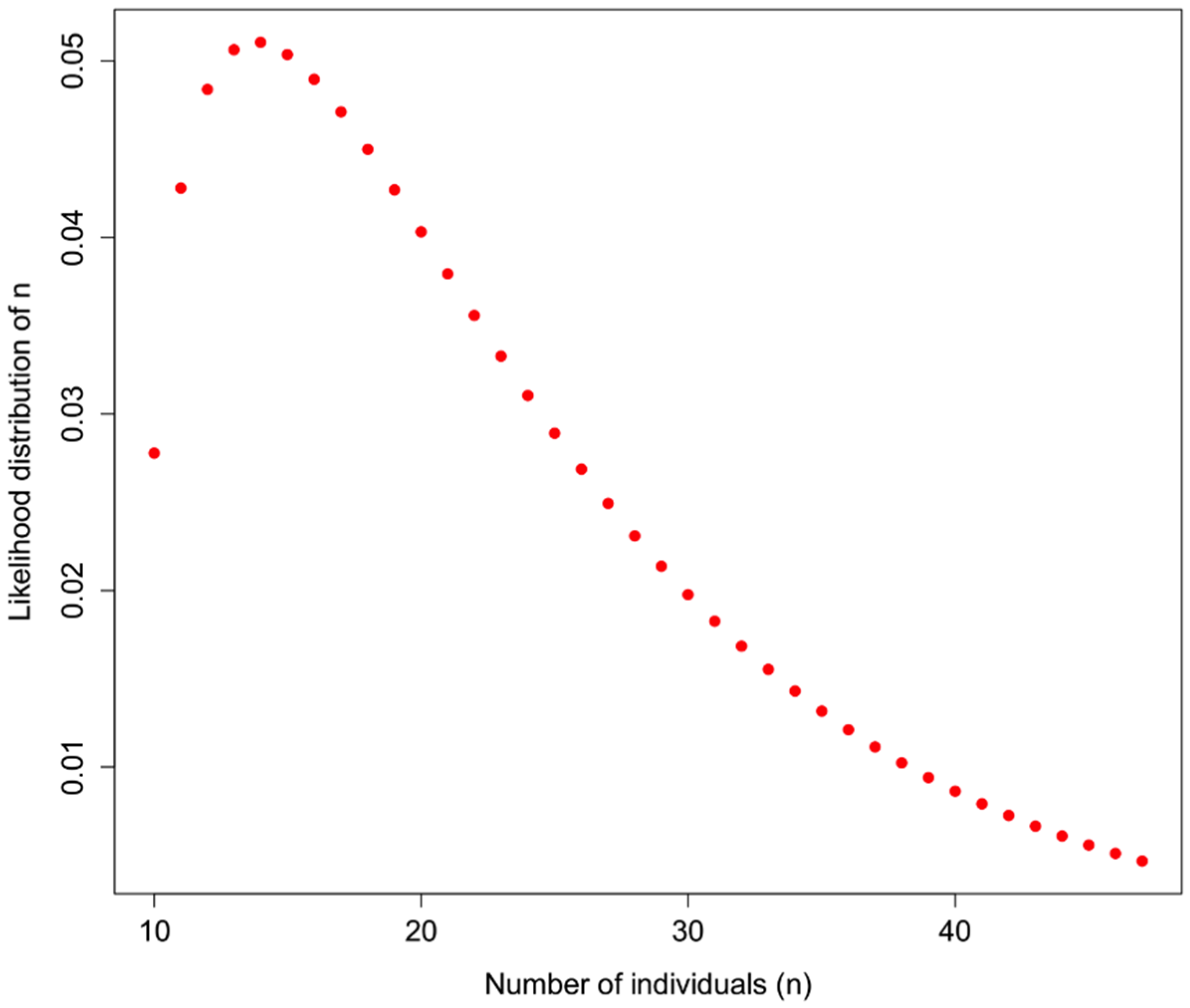
An example of how
H could be used is shown in
Figure 1 for a sample in which 10 distinct haplotypes are observed, and the
prior information about H for a particular taxon is
H = 0.7. In addition to assuming that prior information about the population is appropriately comparable, here we assume a minimum of 10 individuals, and that what we do not know can be modeled by a Gamma distribution with the shape defined by the reciprocal of haplotype diversity (so that low diversity provides little information, high diversity suggests that the number of individuals is closer to the observed number of haplotypes), and the rate is defined by the reciprocal of the number of haplotypes.
Figure 1.
Likelihood of identifying n individuals in a sample in which 10 haplotypes are observed, and the haplotype diversity of the originally observed population is H = 0.7. Here, a gamma function is applied to represent the likelihood such that the distribution is flat at low values of H and a sharper distribution with high values of H, bounded by the actual observed number of haplotypes.
So, observing 10 haplotypes for this taxon, and using the gamma to obtain a useful probability shape based on assumptions about how informative haplotype diversity is, we might feel comfortable believing 14 individuals were sampled (the highest likelihood solution). A concern here lies in the willful abuse of the gamma distribution without a better understanding of how haplotype diversity H and the sample size N may be actually related through the frequency of haplotypes—remember, at this point we are assuming we cannot trust the proportion/frequency representation of an allele in our sample.
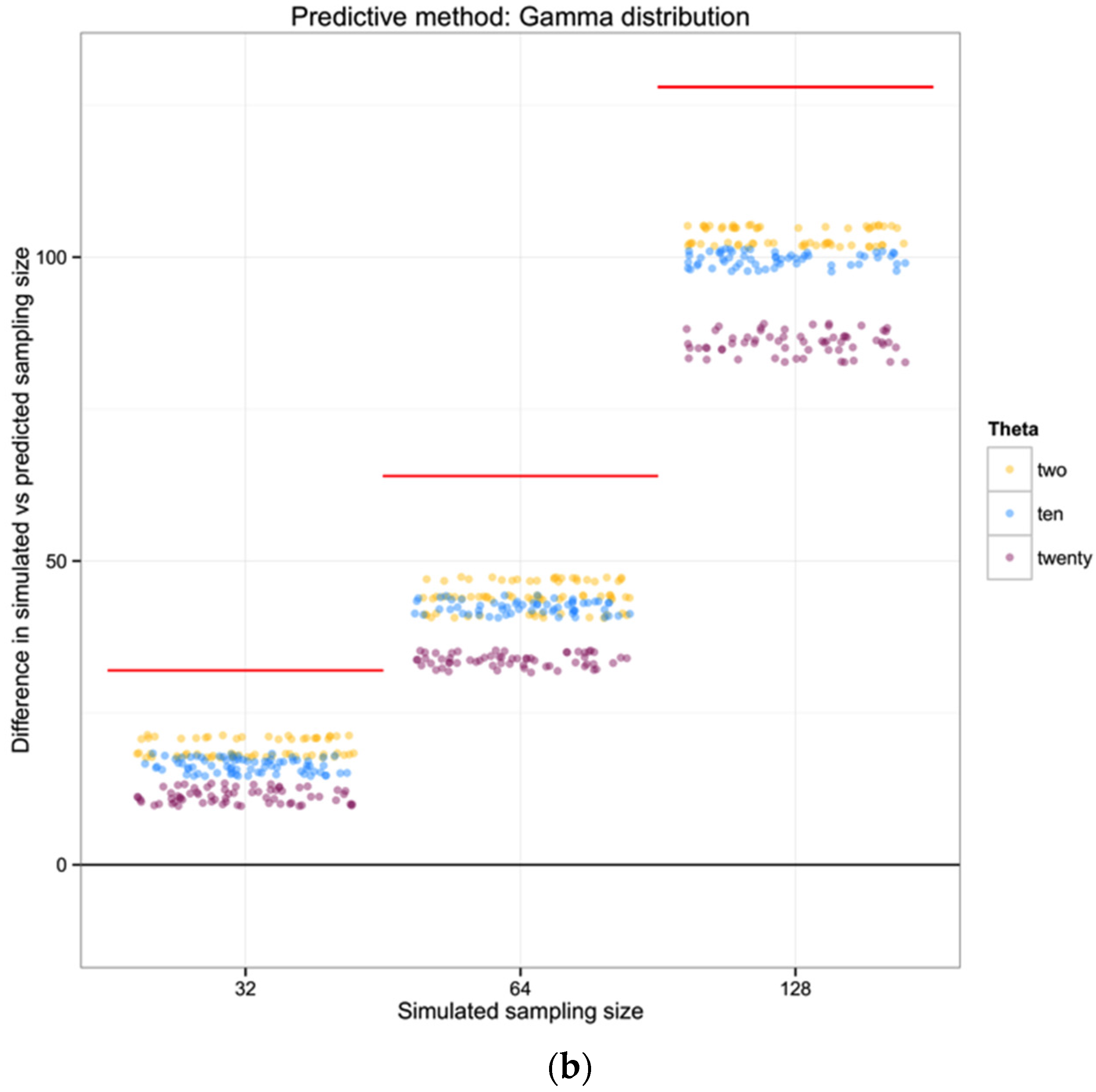
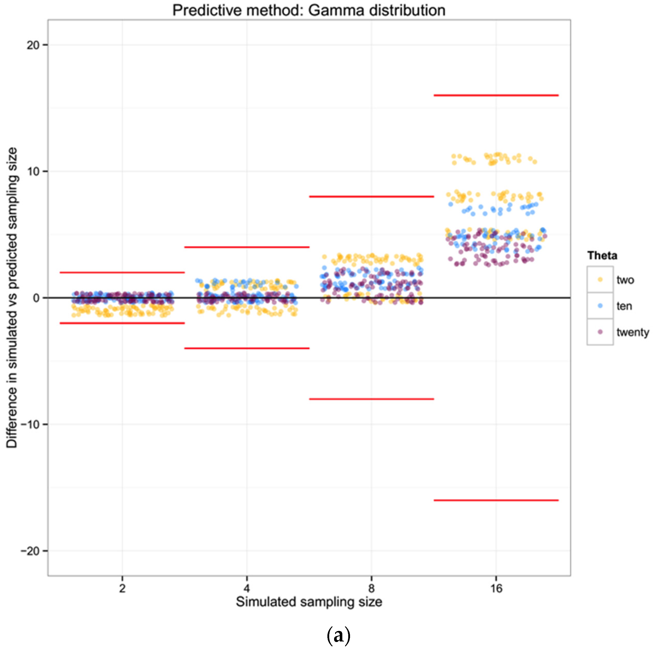
For each of the 100 replicates in each sampling size within the three simulated populations we used the corresponding haplotype diversity for that population and the number of haplotypes observed in that replicate to estimate the likelihoods of the number of individuals in the sample (sampling size) using a gamma function as defined above (shape defined by the reciprocal of haplotype diversity and the rate defined by the reciprocal of the number of haplotypes). From each likelihood distribution we recorded the sampling size with the highest probability to compare with the simulated sampling size in each replicate. Finally, we calculated the difference between the “real” sampling size—the one from our simulations—and the sampling size inferred using the gamma distribution method, as a measure of the precision of our method.
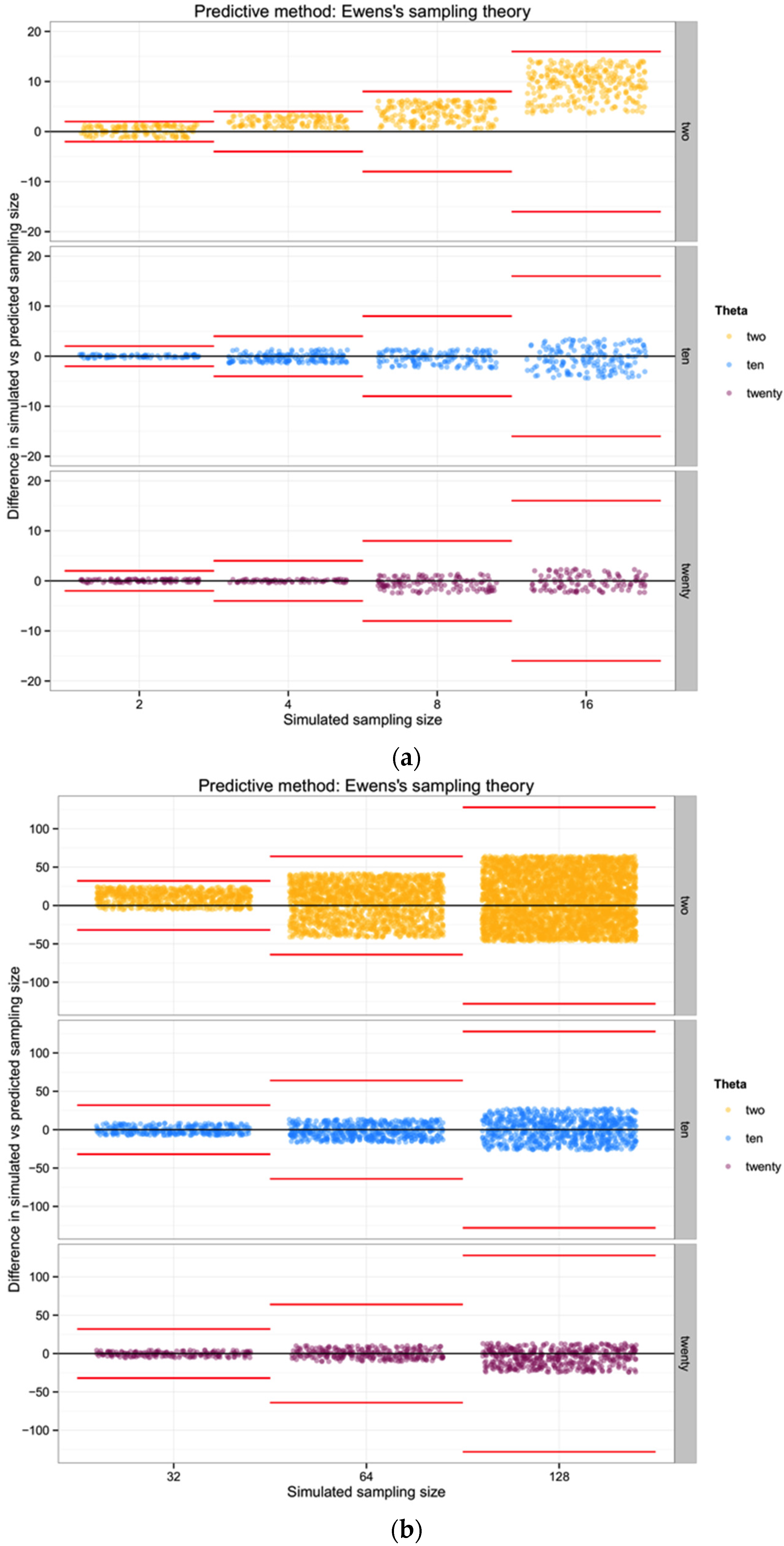
2.2. Sampling Theory
Ewens [
19] developed a sampling theory of selectively neutral alleles, that based on the number of samples and the mutation parameter θ, allows one to estimate the expected number of different alleles (here, we address alleles from a haploid genome,
i.e., haplotypes) in a sample. Assuming a sample of n individuals, the mean number of haplotypes in a sample can be approximated by:
where,
h is the number of different haplotypes in the sample,
n is the number of individuals in the sample, and θ = 4N
eu.
If θ is very small, the expected number of haplotypes should be quite low regardless of the number of individuals sampled. On the other hand, if θ is extremely large, the number of haplotypes should tend to
n as noted above; of course there is a close relationship between Ewens’ sampling theory and our understanding of
H. Using this equation, we can estimate the distribution of the number of haplotypes for different sampling sizes, with a variance:
In general, the variance increases with θ for n of biological interest. Ewens’ derivations rely on the assumption that the sample size is much lower than the actual population size. Considering this approach, rather than one based in haplotype diversity H, may allow us to avoid the problem of uncertain haplotype frequencies in an empirical data set.
For each of the three populations with theta equal to 2, 10 or 20, and through the range of sampling sizes considered in this study (2 to 128) we applied Ewens’ formula to estimate the expected number of haplotypes (and the variance) for each sampling size. We then compared the observed number of haplotypes in each sample with the expected number of haplotypes by Ewens’ formula for each sampling size and estimated the “observed” sampling size in our sample. The accuracy of the method was calculated as the difference between the “real” sampling size—the one from our simulations—and the number of individuals for the sample estimated using Ewens’s method.
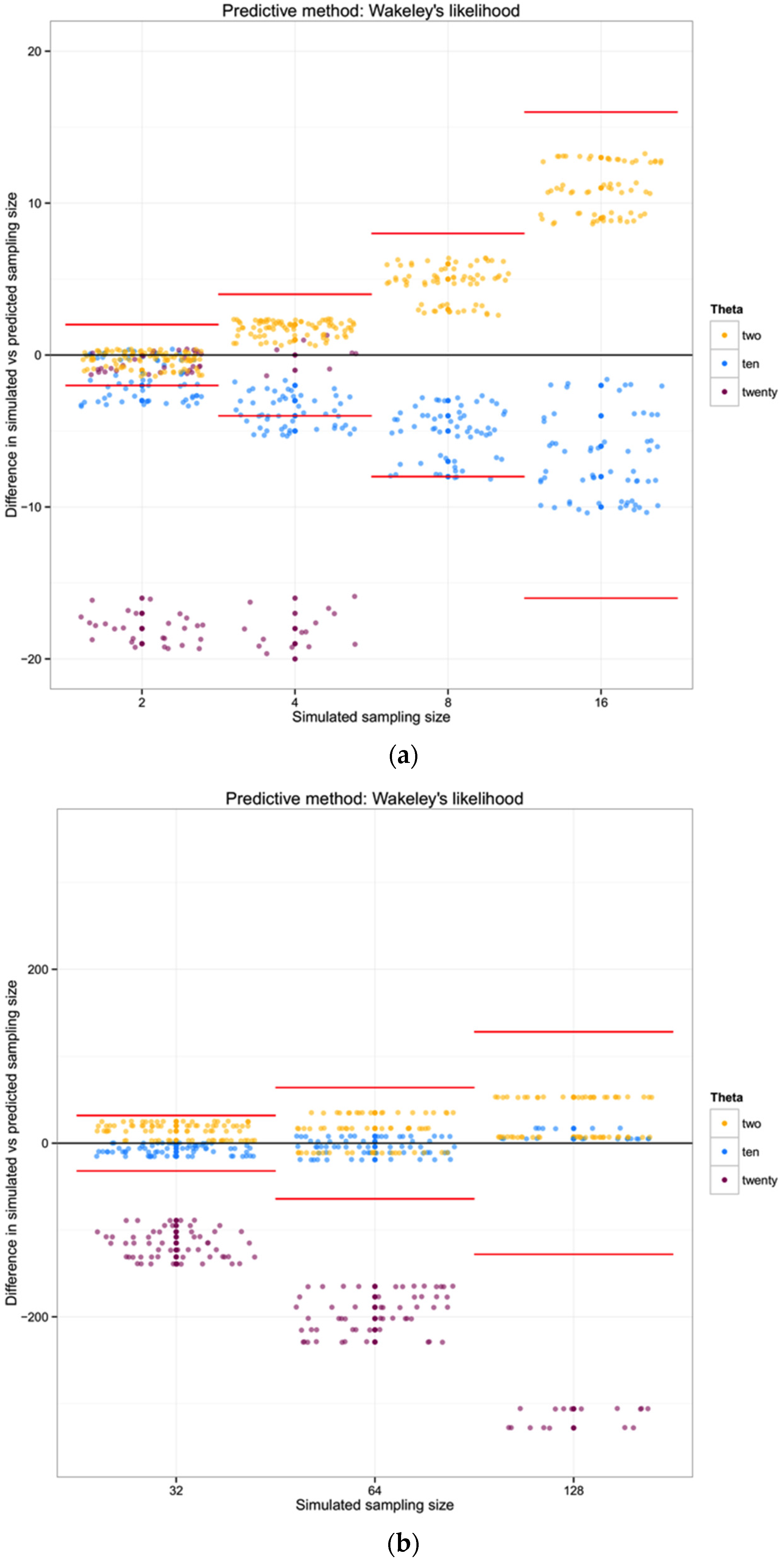
2.3. Segregating Sites
Under the standard coalescent model there are specific probability distributions associated with a sample of sequences, the number of segregating sites
S, and a prior assumption of θ:
Figure 2a illustrates this distribution for θ = 2, segregating sites
k from 1 to 20, and number of individuals
n from 1 to 20. This represents a low-diversity population, and unless few segregating sites are observed there may be a broad range of sample sizes consistent with such an observation.
Figure 2b illustrates the same probability distribution, but assuming θ = 10, with a range of both
k and
n from 1 to 50. When the prior knowledge or assumption of diversity is higher, the range of segregating sites that could give a more accurate inference of
n is higher, with a sharper distribution on
n for lower to intermediate
k.
For each of the three populations with theta equal to 2, 10 or 20, and with a range of sampling sizes from 2 to 128, we applied Wakeley’s [
17] equation 4.3 (presented above) to estimate the expected number of segregating sites for each sampling size. We then compared the observed number of segregating sites in each sample with the expected number of segregating sites for each sampling size and estimated the “observed” sampling size in our sample. The accuracy of the method was calculated as the difference between the “real” sampling size—the one from our simulations—and the inferred number of individuals in the sample.
Figure 2.
Probability surface of observing a number of segregating sites k for a given sample size n when θ is set. In (a), θ = 2; in (b), θ = 10.
Figure 2.
Probability surface of observing a number of segregating sites k for a given sample size n when θ is set. In (a), θ = 2; in (b), θ = 10.
2.4. Comparing Methods
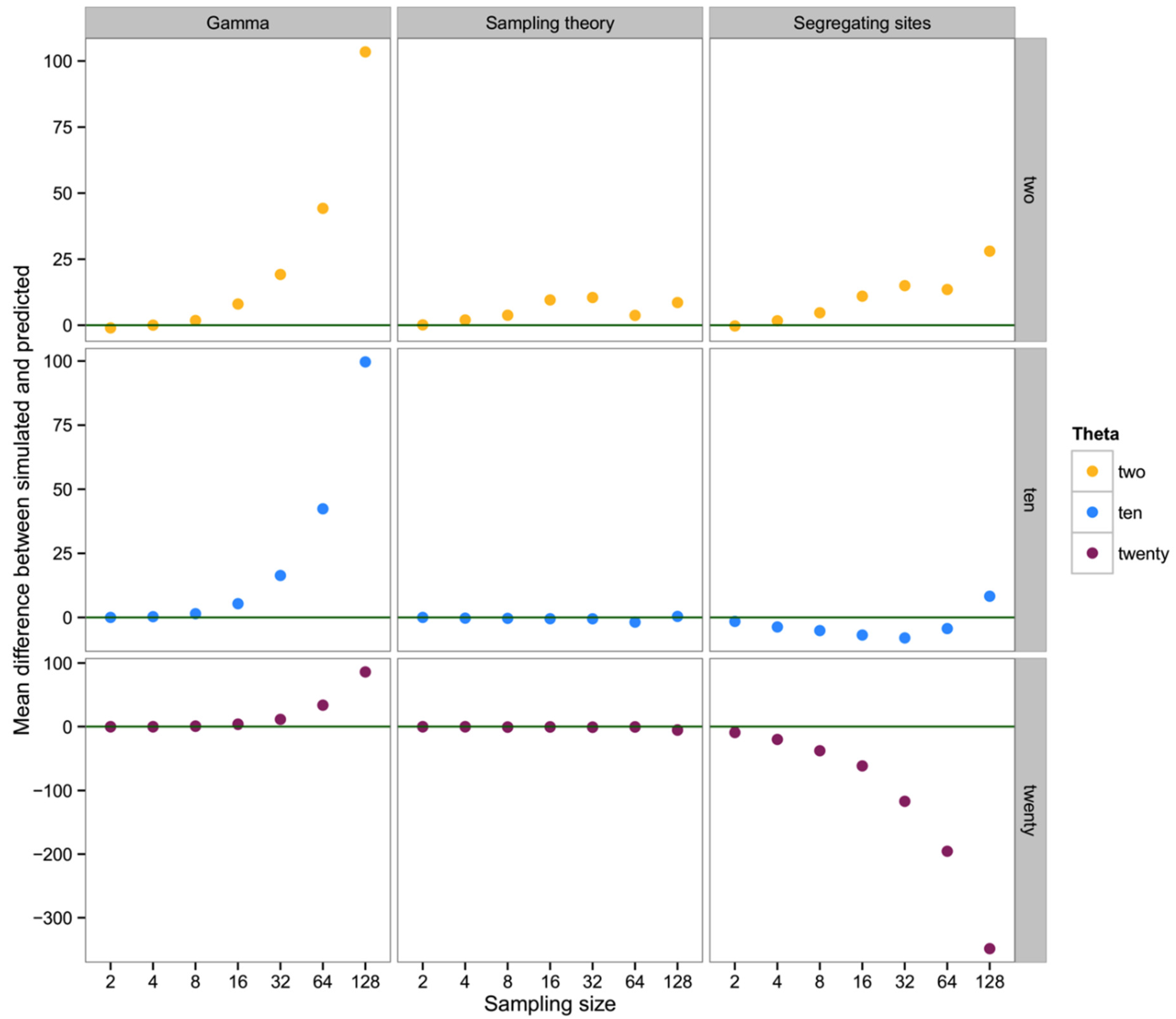
To summarize and compare the three methods we calculated the mean of the difference between simulated and predicted for each combination of θ and type of method.
4. Discussion
What we have shown is, in effect, the high variance in genealogical and mutational data associated with the coalescent process in population genetics [
26]. Though our early efforts suggested a broad utility in ranking the abundance of taxa in a mixed sample of metabarcoding data, the result of our extended simulations indicate a preponderance of high-variance, biased results in estimating the number of individuals in a sequence data set. In considering basic haplotype diversity
H, the observed number of haplotypes, as well as the number of segregating sites
S, attempts to use genetic diversity tend to greatly underestimate the simulated sample of individuals, at least for larger sampling sizes and/or low values of the mutation rate θ. Fundamentally, this problem can be seen in
Figure 2 for θ = 10; although there is an observable and relatively sharp distribution of probability relating a particular number of segregating sites
k for a given number of individuals
n, the surface is quite wide with respects to
n as
k increases for a given θ.
The one component of these summary statistics that indicates an unbiased relationship between θ,
n, and the number of haplotypes is, of course, a simple reflection of Ewens’ [
19] sampling theory. This suggests that
if we already have a good understanding of θ for a particular population (for example if metabarcoding efforts are documenting the mix of individuals in a system that is already well-characterized for most species), then observing a number of haplotypes in a metabarcoding sample allows some nominal indication of how many individuals are likely to have been included. Overall, however, if our goal is to improve the ability to quantitatively describe the biodiversity in a system using metabarcoding approaches, we show that such an approach is of poor utility unless the diversity of the system is high and the number of individuals input to the metabarcoding analysis is modest. Given the additional uncertainty associated with assumptions of comparable diversity from prior evaluation of each population, there are no benefits in cost or estimation over traditional (
i.e., Sanger) barcoding of individual specimens.
Some of the error or bias in estimation we note from our simulation work reflects common problems in sampling data and exploring them with summary statistics. Felsenstein [
27] had noted that a high variance (in fact, driven by bimodal distribution of resultant statistics) in the number of segregating sites
S would be expected with low sample size. Effectively, the comparison of a small number of sequences in a high-diversity system has a large probability of pairwise contrasts across the oldest node of a genealogy [
27], and at very small sample sizes there is a potential that two closely-related sequences are sampled rather than reflect the TMRCA of the genealogy. Additionally, the saturating relationship between sample size and observed diversity has been pointed out by Wakeley [
17] as a feature of efficient estimation of θ from a natural sample; turning the crank on this equation backwards results in an inefficient inference of
n from the other parameters.
Additionally, our approach is predicated on the idea that prior analysis of a given population—a genetically discrete and relatively homogeneous evolutionary unit, which can be difficult to delimit in and of itself [
6,
8,
18]—will effectively suggest the diversity to be found in subsequent samples. There are certainly instances where the diversity at a barcode locus has been so extraordinarily high that haplotype diversity approached 1, and the number of haplotypes recovered in a sample was very close to the number of individuals in that sample, such as the barnacle
Balanus glandula [
28,
29,
30]. However, this same unusual example of a hyperdiverse barnacle also requires recognition that there are at least 2 distinct evolutionary lineages in this taxon with broadly overlapping geographic ranges [
30], which dramatically affects our understanding of the diversity recovered as well as the underlying genealogical process and association with regional diversity. Overall, to obtain accurate estimates of the number of individuals input to a metabarcoding study has proven quite difficult [
9,
31].
In addition to being cautious about identification of the most appropriate reference lineage for study of genetic diversity using these methods, we also note that many loci used in “barcode” studies will deviate from the assumptions of neutral molecular evolution [
15]. Some ribosomal genes, for example, will exist in many copies in a genome [
32,
33]. Additionally, the commonly-used COI gene region for barcoding metazoan communities [
31,
34] is known to exhibit significant effects of purifying selection on the diversity recovered from a population [
35,
36]. Our own modeling work initially included simulations intended to reflect this dynamic in mitochondrial loci (results not shown), but for the sake of clarity we here address only the diversity patterns assuming strict neutrality.
The statistics we evaluate are not independent from one another; they pertain to the same genealogical process assumed to underlie a sample of DNA sequence data and are different ways of summarizing this coalescent process. Although some methods, e.g., approximate Bayesian computation, have been used to infer the demographic history of a sample of sequences using the aggregate of summary statistics available [
37], the relationship shown here appears to be too tenuous to make an advance in our ability to estimate relative abundance of taxa from such metabarcoding data. It does seem that among high-θ populations there may still be comparisons appropriate in a relative sense: greater haplotypic diversity from a metabarcoding sample would suggest more individuals of that species were in the sample. In this way we can evaluate order-of-magnitude results, and have less need for prior information from a population. From the metabarcoding data themselves, each discrete population offers an estimate of θ and a number of observed, distinct haplotypes; this information is likely sufficient to bin abundances into more inclusive groupings of “common”, “intermediate”, and “rare” (e.g., a simplified Preston or Whittaker plot [
38]).


