A Proposed Revision of Diversity Measures

Abstract

The current measures of diversity for vegetation, namely alpha, beta, and gamma diversity are not logically consistent, which reduces their effectiveness as a framework for comparative vegetation analysis. The current terms mix concepts: specifically, while alpha diversity measures floristic diversity at a site, and gamma diversity measures floristic diversity regionally, beta diversity is a measure of diversity between two sites and measures a different phenomenon. We seek to rationalise measures of diversity providing a scalar set of measures. Our approach recognises vegetation diversity extends beyond species diversity and should include the various ways plants express themselves phenotypically. We propose four types of diversity, with a new set of prefixes: Type 1 diversity = the largest scale−the regional species pool; Type 2 diversity = the large habitat scale−where species in a habitat have been selected from the regional species pool; Type 3 diversity = intra-habitat expression of floristics, structure, and physiognomy; and Type 4 diversity = the finest scale of expression of vegetation diversity reflecting site selection of floristics, physiography, and phenotypic expression and reproductive strategy. This proposed framework adds significant new power to measures of diversity by extending the existing components to cover floristics, structure, physiognomy, and other forms of phenotypic expression.

1. Introduction

The current set of diversity measures for vegetation, namely alpha, beta, and gamma diversity, have been used extensively in ecology over the past 40 years [1]. However, practitioners have struggled to provide a consistent set of tools to operationalise these measures to describe vegetation diversity from the regional to local level. We contend this is caused by inconsistencies in the measures which has led to a plethora of interpretations, and has not provided a rigorous framework for comparative vegetation analysis. Tuomisto (2010) clearly identifies the many ways in which the existing diversity measures (indices) have been differently applied leading to confusion [2]. Over the past 30 years that we have been practicing as ecologists, we have been concerned with the use of the diversity measures for a number of reasons. The various terms are mixing concepts:

• alpha diversity is a measure of floristic diversity at a site,
• gamma diversity is a measure of floristic diversity regionally,
• beta diversity is a measure of the diversity between two sites and is trying to measure a different phenomenon from alpha diversity and gamma diversity.

Alpha diversity and gamma diversity can be viewed as expressions of a continuum of floristic composition at different spatial scales. Beta diversity is a measure generally used at the same scale as alpha diversity (viz., the site scale) but is a different concept as rather than directly measuring diversity, it compares diversity. We contend that because it is commonly understood that the terms “alpha”, “beta”, and “gamma” are equivalent to labeling entities A, B, and C, which represent categories of classification ranked along an axis, or a series, or at least represent scalar stages of similar categories [such as vegetation (floristic) diversity], this causes confusion.

This paper seeks to introduce new concepts in the measures of diversity to help provide a scalar set of measures, and to rationalize the diversity nomenclature. While several recent papers have debated the conceptual definitions for different measures of species diversity, they have generally dealt with the measures individually and have not addressed the current inconsistencies in scale and concept embedded in Whittaker’s original diversity measures. In this paper we propose to completely separate the scalar measures of diversity (alpha and gamma) from the comparative measure of diversity (beta), and to then re-order and extend the scalar measures.

In the literature many different mathematical “solutions” have been proposed to operationalise diversity measures, but to date the quantitative definitions have not been universally agreed upon and remain controversial, and no standard set has emerged [3]. Significant progress has been made in better understanding how to measure diversity between sites (beta diversity) and several authors have proposed revisions to help refine this concept [2,4,5,6,7,8,9].

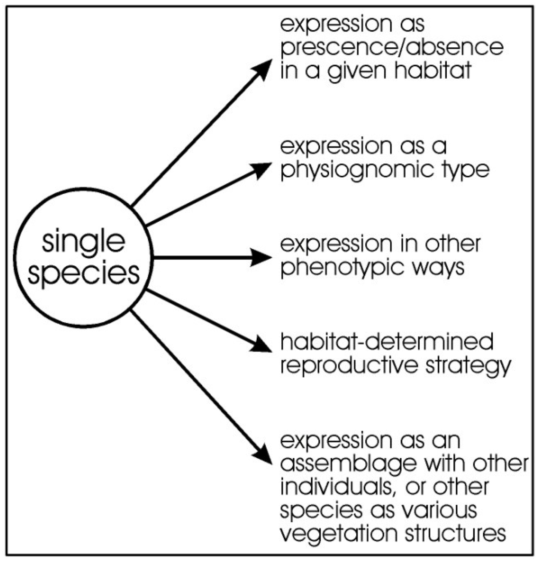
Vegetation diversity extends beyond just the floristic components and should include the various ways a plant species expresses itself phenotypically and, therefore, the concept itself needs to be broadened (Figure 1). We consider all expressions of a species to be part of “diversity”. Measuring diversity requires more than simply measuring diversity as species richness.

In this paper, the term habitat refers to the abiotic space that biota occupy developed by smaller scale geomorphology, substrate, groundwater and soilwater salinity, or a hydrological interface. It is the sum of the physico-chemical factors that determine whether a given location is inhabitable by biota. It is used here solely to refer to the abiotic “environmental space” which is then utilised by a common recurring set of plants and animals. For mangrove habitats, discussed later, the term is largely synonymous with a small-scale geomorphic unit with a specific substrate, tidal level, and hydrochemistry.

Figure 1. Idealised diagram showing how the pressures on a species drawn from the regional species pool and how the environment can select for species presence/absence, determine its expression physiognomically and other ways phenotypically, and together with other individuals of the species, or from other species, can generate floristic occurrence, physiognomy, vegetation structures, and phenology.

Figure 1. Idealised diagram showing how the pressures on a species drawn from the regional species pool and how the environment can select for species presence/absence, determine its expression physiognomically and other ways phenotypically, and together with other individuals of the species, or from other species, can generate floristic occurrence, physiognomy, vegetation structures, and phenology.

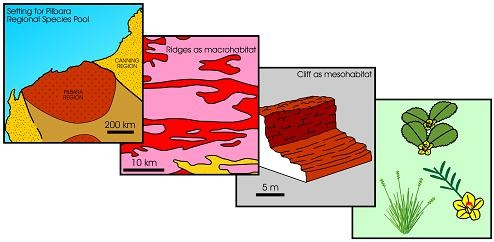
Habitat can be treated in a scalar manner. The larger scale habitats, for instance such as rocky ranges as distinct from alluvial plains, or broad tidal flats, or coastal spits, are termed macro-habitats. These habitats can be progressively subdivided into finer-scale features, and these are meso-scale, and micro-scale habitats, or meso-habitats and micro-habitats. Thus, for example, a rocky range may be subdivided into meso-habitats of cliffs, rocky outcrops, scree, and soil-covered inter-outcrop flats, and a spit can be subdivided into meso-habitats of gravelly mid-tidal slope and sandy high-tidal slope. At the next scale down, rocky outcrops may have micro-habitats of bare rock surfaces, creviced rock surfaces, and soil-filled crevices, while spits may have gravelly mid-tidal slopes differentiated into micro-habitats on bases of soil moisture and salinity.

While we are aware of the importance of herbivory, fire, and other natural and anthropogenic disturbances to the selection and shaping of plant species in terms of their assemblage composition, physiognomy, structure, and phenology at different scales [10,11,12,13], we have focused only on the abiotic factors that determine plant ecology to simplify the discussion on the classification, comparisons, and ecologic controls on vegetation. As such, this paper emphasises the physico-chemical features of the habitat and its role in primary selection of species from the regional species pool, and develops the idea that there is a response of flora to ecological pressures, underpinned by physico-chemical processes and products at progressively finer habitat scales that result in various expressions of biodiversity.

Theoretically, a given habitat, with its specific edaphic factors, may select for some species (from the regional species pool) and eliminate others, thereby forming assemblages with specific floristic composition. The regional species pool is here used in the sense of the total species that exist in a given region, where a region is defined by a distinctive geology, landscape, soils, hydrology, and climate. While there may be overlap in species content at the boundaries of different regions, we imply here that the boundary of a regional species pool often is defined by a change in abiotic setting that defines a given region. For example, three adjoining regions in Western Australia, viz., the Pilbara Region of rocky uplands of ironstone, volcanic rock, and granite, and alluvial tracts, the Great Sandy Desert Region of linear desert dunes, and the Kimberley Region mainly of sandstone plateau, are identified by their geology, landscapes, and climate [14,15]. Floristically, in Western Australia, the regional species pool of the Pilbara region is different from that of the Great Sandy Desert, and from the Kimberley Region. The boundaries between areas identified as “regional species pools” may be relatively sharp if controlled by geology and landscape, but may be more diffuse if controlled mainly by climate. Regional species pool viewed by other authors denotes a defined region of species from which each member of the pool can potentially colonise every local site within a biogeographic region [16,17,18]. The term “regional species pool” is broadly equivalent to the concept of a “bioregion” in Australia which Thackway & Cresswell (1995) define as “relatively large land areas characterised by broad, landscape-scale natural features and environmental processes that influence the functions of entire ecosystems”, and to the species-indicative biogeogeographic regions of Western Australia [19,20].

At finer scales, environmental factors determine the species form, and whether they develop into forests, heaths, or other structural forms and, at still finer scales, whether the species responds to the environment in various physiognomic ways (as single-trunked trees, as gnarled, recumbent trees, or multi-stemmed shrubs, or a dwarf plants, and so on). Indeed these same abiotic factors determine how each species maintains its populations by various sexual or asexual strategies (seed production, epicormic shoots, “layering”, shoots emanating from root networks). All of these expressions of plant life, from the regional level in terms of floristic composition to the very local level in terms of selected species composition and their structure, physiognomy, and small scale phenotype; are expressions of diversity.

2. Examining the “Sequence” of Alpha, Beta, Gamma Diversity

It is commonly understood that a sequence of terms such as alpha, beta, and gamma represents some form of series, a “numerical” gradient or a “ranked” gradient, where the ranking reflects a gradient of categories. Generally, in science, such a ranking proceeds from the large scale down to the small scale, or vice versa. The sequence of Greek letters, alpha, beta, gamma, delta, epsilon, etc., is often used in science as adjectival descriptors to designate gradients, sequences, and series. In Euclidean geometry the order of notation of angle in a triangle is A, B, C and the Greek versions, alpha, beta, gamma, are also sometimes used [21]. Another example is the Bayer method of systematic star nomenclature [22]. For the most part, Bayer assigned Greek letters to stars in rough order of apparent brightness within a particular constellation. The stars were named by assigning a constellation name and applying a Greek letter (alpha, beta, gamma, delta, epsilon) in an approximate order of decreasing brightness for the stars in that constellation (though there are exceptions).

Metallurgically, the crystalline phases of iron, in response to increasing temperature, once were noted as alpha Iron, beta Iron, gamma Iron, delta Iron (beta Iron is largely an obsolete term because it is crystallographically similar to alpha Iron and is considered now to be the high-temperature end of the alpha phase field) [23]. In chemistry, the four tocophenol and four tocotrienols forms of Vitamin E occur in alpha, beta, gamma, and delta forms, and are labelled as alpha-tocopherol, beta-tocopherol, gamma-tocopherol, and delta-tocopherol, and so on [24], the series corresponding to the position and general decrease in methyl groups, and increase in OH.

We contend that for vegetation the “gradient” should be named with prefixes to reflect the most species-rich category down to the most species-depauperate category, i.e., from the regional species pool, representing the maximum number of species available, to the more limited number of species selected by the habitat and microhabitat. Significantly, the gradient should not mix conceptual categories.

3. Ranking of Diversity

Ranking of diversity should begin at the largest scale, or regional scale (with the greatest opportunity of floristic expression embedded at this scale), with later progressive categories derived (or determined) by habitat selection or environmental pressures, with species drawn from the regional species pool and their physiognomy and vegetation structure determined by finer scale environmental pressures.

A ranked set of diversity measures could ideally be labeled alpha, beta, gamma, and delta as prefixes to the term “diversity”. However, the prefixes alpha, beta, and gamma, as presently used, are firmly entrenched in the literature with alpha diversity and gamma diversity having broadly conceptually similar meaning to what we propose but in reverse order of scale, and with beta diversity with a completely different conceptual meaning altogether. This historical precedent precludes our use of the prefixes alpha, beta, gamma, and delta.

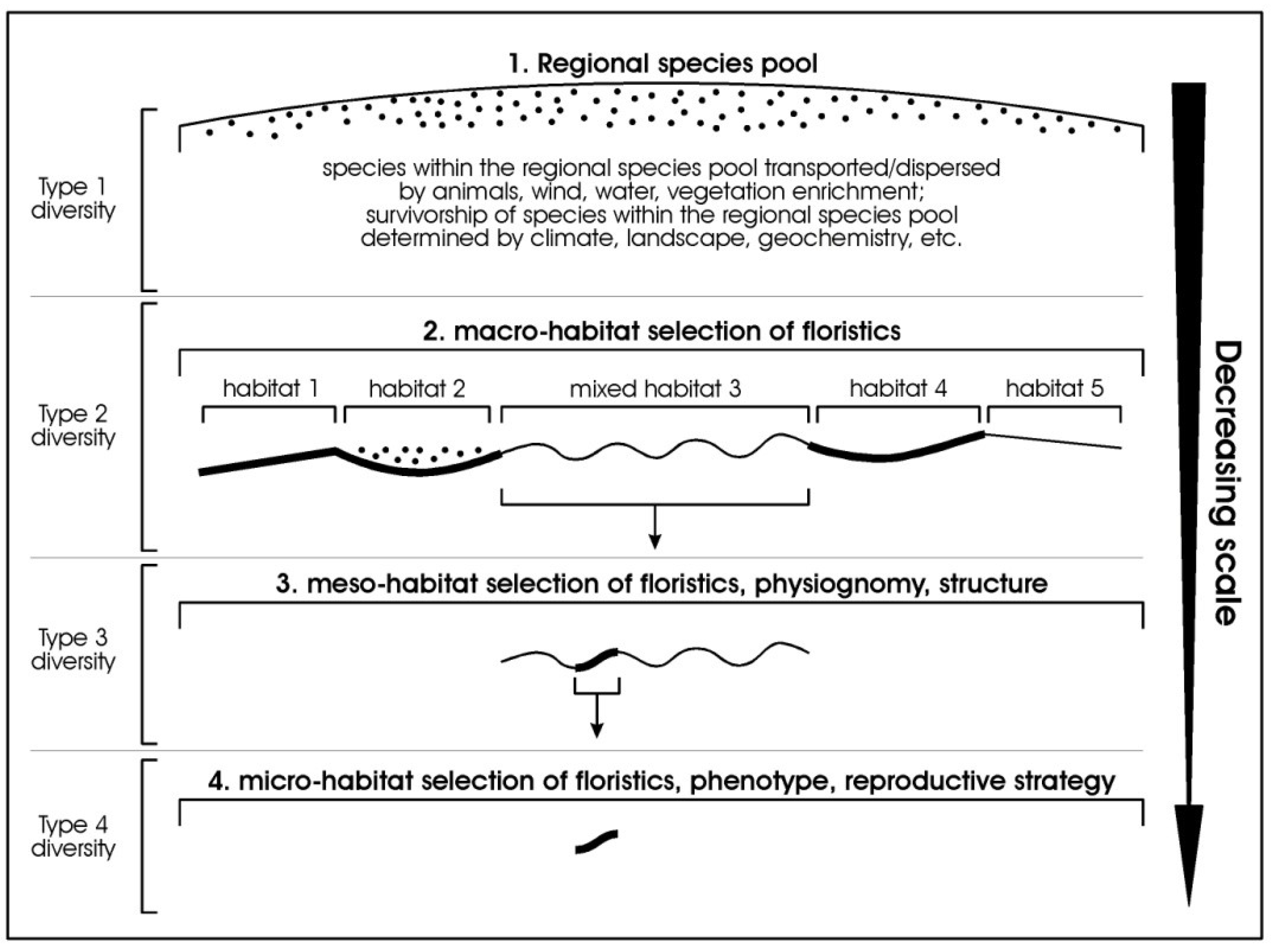
To convey our ideas of grading diversity from the large scale to the finest scale, as suggested above, we propose a new set of prefixes, Type 1 to Type 4, representing the sequence of grades, and illustrated in Figure 2.

• Type 1-diversity = the largest scale—the regional species pool (equivalent to gamma diversity of Whittaker);
• Type 2-diversity = the macro habitat scale—where species in a broad habitat have been selected from the regional species pool;
• Type 3-diversity = intra-habitat expression of floristics, structure, and physiognomy (in part equivalent to the floristic alpha diversity of Whittakers);
• Type 4-diversity = the finest scale of expression of biodiversity (in part equivalent to the floristic alpha diversity of Whittaker, depending on scale of site description).

While within the four tiered system proposed there are equivalents to the original schema proposed by Whittaker (1972) [1], this proposed system re-orders the terms to proceed from the largest scale to the smallest scale, introduces a new term to deal with diversity at the macro-habitat scale, and includes diversity of physiognomy and structure. Importantly, by explicitly linking the measures to a known scale it allows for direct comparison of like with like (currently termed beta diversity, but applied at multiple scales and not just at the site-scale).

Figure 2. Idealised diagram showing progressive decreasing change of scale for a regional species pool to macro-scale habitat-selected floristics, to meso-scale habitat-selected floristics, physiognomy, structure, and phenology, to micro-scale habitat-selected floristics, phenology, and reproductive strategy. Five idealised habitats are illustrated at the macro-habitat level.

Figure 2. Idealised diagram showing progressive decreasing change of scale for a regional species pool to macro-scale habitat-selected floristics, to meso-scale habitat-selected floristics, physiognomy, structure, and phenology, to micro-scale habitat-selected floristics, phenology, and reproductive strategy. Five idealised habitats are illustrated at the macro-habitat level.

This proposed system adds significant new power to the measures of diversity by introducing new components other than floristics and thus providing measures of diversity that address floristics, structure, physiognomy, and other forms of phenotypic expression in comparative measures between sites. The need for a classification system that addresses vegetation features beyond floristics is recognised by systems where broad floristics is combined with vegetation structure [25,26,27].

An additional outcome of this new schema is that comparative analysis of diversity between places or sites (beta diversity) is made more rigorous. The comparison of two sites, regardless of their scale, can be undertaken if the comparisons are carried out at the equivalent scales. Regions can be compared in terms of species composition, i.e., Type 1 diversity from one region can be compared with Type 1 diversity from another, and Type 2 diversity from one large scale habitat can be compared with Type 2 diversity from another, and so on. The principles of comparative beta-diversity [1,28] can be applied to the measures and results of Type 1 diversity, Type 2 diversity, Type 3 diversity, and Type 4 diversity. This will provide greater clarity to the possible types of beta diversity (and the framework needed to utilize them within) as discussed by Anderson et al. [28].

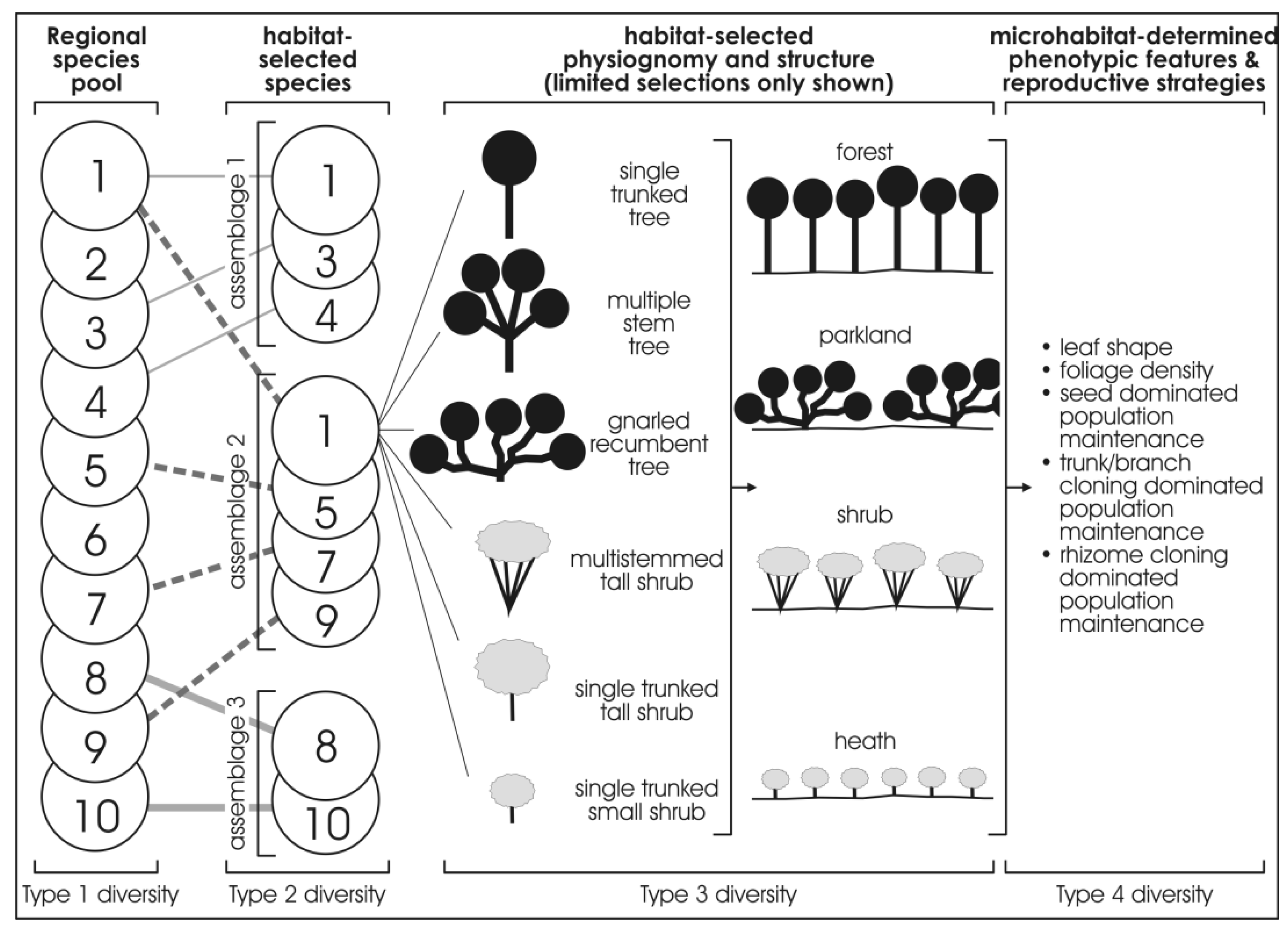
Figure 3 provides a more detailed illustration of the four types of diversity. The first column (Type 1 diversity) represents the regional species pool, which is purely the species richness of a region which can be described as the “umbrella of species availability”. In any given region, it is the whole complement of species that inhabit the various habitats that occur in that region. Thus, for instance, in Western Australia, the regional species pool of the Pilbara region with 2020 species of flora, differs from that of the Great Sandy Desert with 1,680 species of flora, and from the Kimberley Region, with 2,080 species of flora, and the Stirling Range with 1,500 species of flora (many of which are endemic to the Stirling Range), or the South-Western region with 5,710 species of flora [19,20,29,30,31,32,33,34,35,36,37,38,39,40]. Adjoining regions may overlap in species content in their pool of species.

Figure 3. Idealised diagram showing progressive selection from the regional species pool (the species numbers used in the regional species pool amount to ten, but it could be 100 species or 1000 species), a range of habitat-selected species which, in turn, progressively are selected as to physiognomy, other phenotypic expressions, and vegetation structure.

Figure 3. Idealised diagram showing progressive selection from the regional species pool (the species numbers used in the regional species pool amount to ten, but it could be 100 species or 1000 species), a range of habitat-selected species which, in turn, progressively are selected as to physiognomy, other phenotypic expressions, and vegetation structure.

The second column (Type 2 diversity) represents the habitat-selected species that occur in a given habitat in a region. Thus, for instance, using extremes of habitats, in the Pilbara region, from the 2,020 species of flora in the regional species pool, some 20 species inhabit basin clay-floored wetlands, some 10 totally different species inhabit narrow shale ledges on rocky hills of the region, and about four totally different species inhabit ironstone cliffs on these rocky hills. Again, as for Type 1 diversity, Type 2 diversity captures only the species richness of a given habitat.

The third column, (Type 3 diversity) represents a finer scale of habitat-selected floristics, physiognomy (the shape of a plant) and the structure of the vegetation for the species that occur in a given habitat. For example, the one species may occur in physiognomic forms of small slender-trunked shrub, or a small multi-stemmed-trunked shrub, or gnarled small tree in the various habitats that have selected it, resulting in different expressions of vegetation structure (viz., forests, or scrub, or heath, etc.). Each of the species in a given habitat may have a different expression of physiognomy and structure. One species in a given habitat can be expressed as a heath of small multi-stemmed-trunked shrub while another species forms tussocks in an open grassland structure.

The fourth column, (Type 4 diversity) represents the microhabitat-selected phenotypic responses and reproductive strategies for the species that occur in the various micro-habitats. Thus, for example, a given species has varied expression of foliage density, or leaf size, or reproductive strategy in the different micro-habitats.

The gradient of diversity from Type 1 to Type 4 commences with species richness (Type 1 diversity and Type 2 diversity) and progresses to physiognomic and phenotypic expressions (Type 3 diversity and Type 4 diversity).

4. Describing a New Framework for Measuring Diversity

The first major construct that needs to be addressed in any set of measures is scale, moving from the largest scale down to the smallest. Noss (1990) proposed a spatial hierarchy of biodiversity moving from the regional to the individual organism to help measure biodiversity for environmental management [41]. He proposed four levels:

(1)

Regional Landscape

(2)

Community-Ecosystem

(3)

Population-Species

(4)

Genetics.

Similarly, we contend it is necessary to progress from the regional to the local scale, and propose four graded categories of diversity, focused on floristics at the largest scale and then progressively focusing on the outcome of habitat-selection of species and, in turn, vegetation structure, physiognomy, other phenotypic expressions, and reproduction strategies of these species at finer scales. It is at these finer scales that habitat and environmental pressures select species from the regional species pool and determine how they are expressed in the environment:

In terms of scale, the following four types of diversity are proposed:

• Type 1 = the regional scale—an expression of the total floristic diversity or floristic richness of the region;
• Type 2 = the macro habitat scale—an expression of the floristic diversity or floristic richness as expressed in (floristic) assemblages within the (macro-) habitats of the region where species in a habitat have been selected from the regional species pool and find expression in floristic assemblages or even in monotypic stands within a given habitat;
• Type 3 = within the scale of a given habitat—an intra-habitat expression of the diversity of floristics, structure, and physiognomy of vegetation; the species in an assemblage may manifest different physiognomy and structure (e.g., in a mangrove assemblage of three species, one species forms canopy-emergent slender tall single-trunked trees, another forms a closed low forest of gnarled/recumbent individuals, and a third forms multi-stemmed low shrubs or, all species may form a closed low forest each occurring as tall slender single-trunked trees);
• Type 4 = the micro-habitat scale, an expression of the further selection of floristics, as well as physiography, and phenotypic features and reproductive strategies; it is the finest scale of expression of vegetation diversity reflecting intra-habitat microhabitats; there are a wide range of phenotypic responses driving this diversity, including leaf shape, foliage density, branching style, whether population maintenance of a given species in the assemblage are seed dominated, trunk/branch cloning dominated, or rhizome cloning dominated.

There are two major gradients in this graded sequence of categories. Firstly, at a regional level there is a decrease in species richness, from Type 1 to Type 4, where all species are present in the regional species pool to where only environmentally selected species are present in the local habitats within the region. This scalar concept for Type 1 diversity grading to Type 2 diversity in the “selection of floristics” by the abiotic features of the macro-habitats is similar to the concept provided by [18] wherein, on a regional scale, different assemblages of species may develop at different sites, because of the various abiotic conditions that provide the various templates on which community structure will develop. Secondly, at the habitat level within Type 3 to Type 4, there is an increase in phenotypic, physiognomic, and structural expression and complexity as various habitats and environmental gradients determine the differential and various plant expressions of species according to the individual plasticity of their genotype and phenotype.

In order to illustrate that measurement of species diversity alone is inadequate to capture the true variation in vegetation diversity in the real world, an example of mangrove vegetation is provided. Capturing the diversity in vegetation floristics, physiognomy, and structure such as illustrated in these examples will provide a more robust measure of the broader diversity in biodiversity.

Mangrove species are subject to extremes in inundation, water-logging, salinity, and soil types, all of which affect plant physiognomy (plant shape and height, resulting in the one species varying from trees to shrubs to dwarf plants, with single stems to multi-stems to gnarled, recumbent individuals), and vary the ratio of above ground to below ground biomass, reproduction strategies, foliage development, and plant productivity. In the Kimberley Region, which is in a ria coastal setting comprising six main mangrove habitats, with a total of 15 mangrove species [42], the prevailing climate and abiotic habitat drivers combined with a limited regional species pool results in repetitive floristic assemblages of mangroves. Abiotic drivers result in a limited set of species expressed as forests, gnarled-tree parklands, scrub, heath, and stands of dwarf plants, containing both mixed species and single species stands [43].

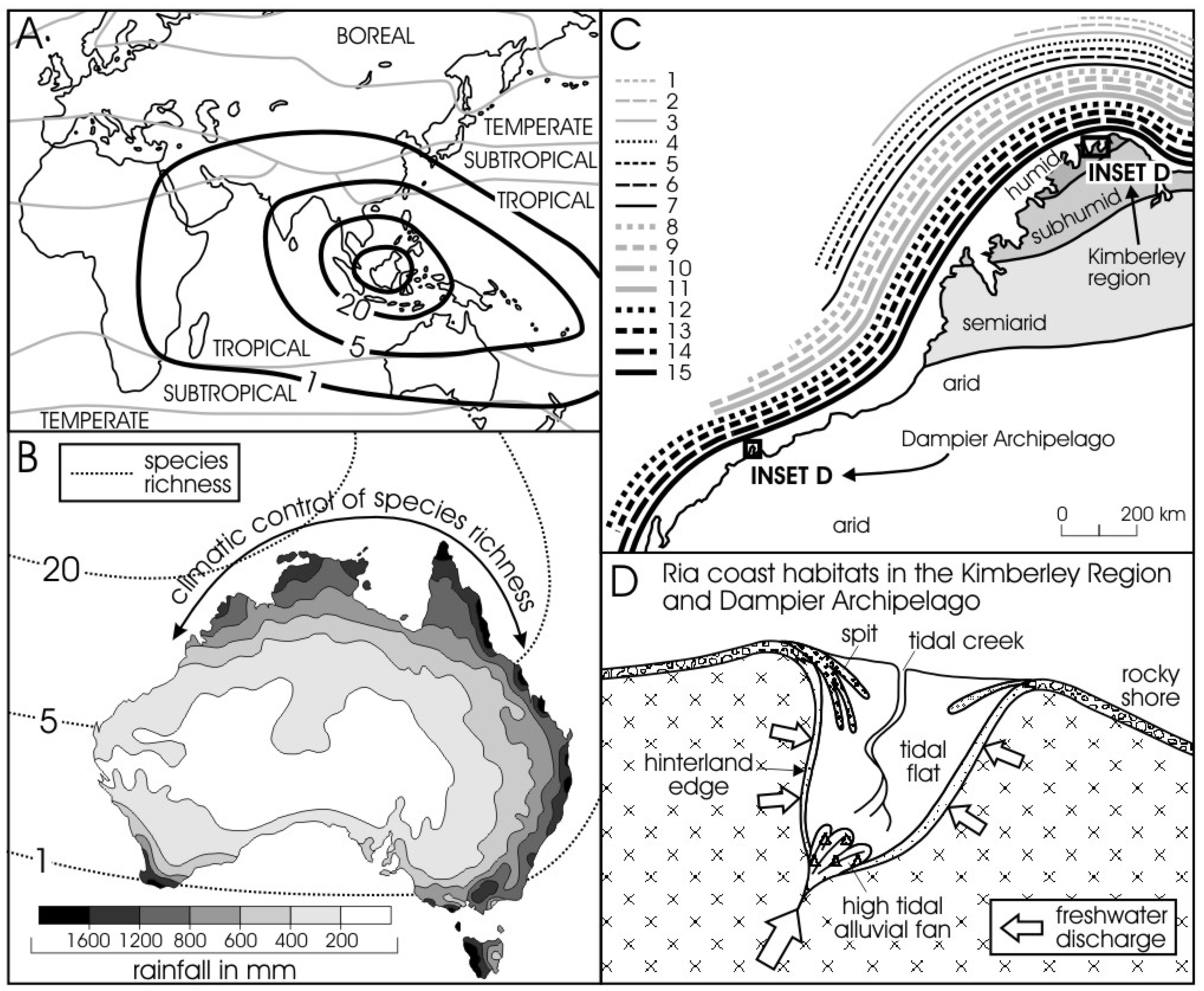
Figure 4 shows the Type 1 diversity in insets B & C, where the species richness in mangroves consists of 10–15 species (as the periphery of the sub-continental gradient of species-rich area of mangroves centered on the Malaysian region, inset A), graded in decreasing abundance (decreasing species richness) from north to south in response to a climate gradient. Within the regional pecies pool (Type 1 diversity) of the Kimberley Coast and the Dampier Archipelago in the Pilbara Region, local embayments with their six habitats select from the pool those species that will inhabit the rocky shores, spits, tidal flats, tidal creek, hinterland edge, and tidal-tidal alluvial fan (Figure 4D). These species on the individual habitats manifest Type 2 diversity, and the composition of these assemblages can be analysed as Type 2 diversity. Figure 4D is an idealised map illustrating the recurring pattern of macro-habitats in ria coast settings (based on [42,44]). Semeniuk (1985) presents quantitative data on the composition of the assemblages that occur on each of these six habitats [44]. The next stage of determining/assessing diversity is identifying structure and physiognomy of an assemblage. We have not progressed to this level for mangroves in this paper, but Semeniuk & Wurm (1987) present information on the structure and physiognomy of each mangrove compositional assemblage (the Type 2 diversity) in a ria coastal setting in Western Australia [26].

Figure 4. Mangroves in the Kimberley Region and Dampier Archipelago of Northwestern Australia. From a regional species pool involving ~20 mangrove species (Insets A & B), there is progressive decrease in the species richness correlated with climate (Inset C); each line parallel to the coast shows the biogeographic distribution of the 15 mangrove species in the Kimberley Region and the six mangrove species in the Dampier Archipelago [Key to numeration of species: 1. Scyphiphora hydrophylacea, 2. Xylocarpus granatum, 3. Bruguiera parviflora, 4. Camptostemon schultzii, 5. Lumnitzera racemosa, 6. Xylocarpus moluccensis, 7. Sonneratia alba, 8. Excoecaria agallocha, 9. Osbornia octodonta, 10. Aegiceras corniculatum, 11. Bruguiera exaristata, 12. Ceriops tagal, 13. Aegialitis annulata, 14. Rhizophora stylosa, 15. Avicennia marina]. Inset D whose geographic locations are shown in (C) for the Kimberley Region and Dampier Archipelago illustrates the range of habitats in these ria coasts. The species richness and structure of the mangrove vegetation in these six habitats of ria coasts is described in [26] and [45].

Figure 4. Mangroves in the Kimberley Region and Dampier Archipelago of Northwestern Australia. From a regional species pool involving ~20 mangrove species (Insets A & B), there is progressive decrease in the species richness correlated with climate (Inset C); each line parallel to the coast shows the biogeographic distribution of the 15 mangrove species in the Kimberley Region and the six mangrove species in the Dampier Archipelago [Key to numeration of species: 1. Scyphiphora hydrophylacea, 2. Xylocarpus granatum, 3. Bruguiera parviflora, 4. Camptostemon schultzii, 5. Lumnitzera racemosa, 6. Xylocarpus moluccensis, 7. Sonneratia alba, 8. Excoecaria agallocha, 9. Osbornia octodonta, 10. Aegiceras corniculatum, 11. Bruguiera exaristata, 12. Ceriops tagal, 13. Aegialitis annulata, 14. Rhizophora stylosa, 15. Avicennia marina]. Inset D whose geographic locations are shown in (C) for the Kimberley Region and Dampier Archipelago illustrates the range of habitats in these ria coasts. The species richness and structure of the mangrove vegetation in these six habitats of ria coasts is described in [26] and [45].

A comparative ria coastal setting is in the Dampier Archipelago area in the arid Pilbara Region [45], where there are seven mangrove species (though only six in the Dampier Archipelago), and the same (six) types of habitats [26].

Tables S1 and S2 (in the supplementary) present information on mangroves in a ria coastal setting in the Kimberley Region, where the regional species pool comprises 15 species of mangroves, and in the Dampier Archipelago of the Pilbara Region, where the regional species pool comprises seven species of mangroves. Each ria coast setting has six mangrove habitats. Tables S1 and S2 show the components of biological expression (floristically, physiognomically, structurally, and phenotypically) for each scalar level of diversity.

In order to better define the vegetation diversity present in this mangrove system, current measures of species diversity (as species richness) alone are inadequate (i.e., alpha, gamma diversity), and indeed, also inadequate for comparisons of species diversity between sites (beta diversity). What are required are measures that also capture the diversity of phenotypic and physiognomic expression. New measures of vegetation diversity, as expressed by species responses to differences in habitat, and which indeed may reflect differences in other elements of biodiversity mostly undescribed or surveyed (e.g., microbiota) are required.

5. Conclusions

We contend that no consensus has been reached on the application of diversity measures because it is confusing and, therefore, propose a new schema. While previous authors have tried to provide a way through the existing terms [2,4,6], the fundamental conceptual flaws, mixing of concepts, and the use of prefixes that are not in fact fully sequential, leads us to conclude it is time to put the measures of diversity into a more structured and logical frame, while also expanding the concept to better include all expressions of vegetation diversity.

Jost (2007) provides a useful review of the derivation of the current set of mathematical equations used to estimate alpha, beta, and gamma diversity [3]. Hoffmann & Hoffmann (2008) correctly point out that regardless of the mathematical expression used to elucidate the theoretical construct of diversity, it is only as good as the input properties to those equations [19]. It is perhaps folly to believe that any single set of measures of our component of biodiversity will provide a representation of true diversity, however, our schema is presented to hopefully lessen the existing confusion and to provide a more structured and logical set of measures to help express the diversity that exists in nature.

The approach of utilizing the Whittaker concept of beta diversity, i.e., comparison between sites of site-specific data, can be applied to the various levels of diversity proposed in this paper. That is, Type 1 Diversity in a given region can be analysed and compared with Type 1 Diversity in another region, Type 2 Diversity in a given region can be analysed and compared with Type 2 Diversity in another region, and so on. For instance, Tables S1 and S2 of this paper, if presented in a quantitative manner, and Table 6 of Semeniuk (1985) [44], which provides quantitative information on the composition of mangrove assemblages within the ria coast habitats, could be used as the basis for comparison between the mangroves in a ria coast in the Kimberley Region and those of a ria coast in the Pilbara Region, though we have not gone to this next level of analysis in this paper.

While this paper has confined its discussion to the application of diversity measures to vegetation, the concepts can be applied more broadly to all elements of biodiversity.

References

- Whittaker, R.H. Evolution and measurement of species diversity. Taxon 1972, 21, 213–251. [Google Scholar] [CrossRef]
- Tuomisto, H. A consistent terminology for quantifying species diversity? Yes, it does exist. Oecologia 2010, 164, 853–860. [Google Scholar] [CrossRef]
- Jost, L. Partitioning diversity into independent alpha and beta components. Ecology 2007, 88, 2427–2439. [Google Scholar] [CrossRef]
- Jurasinski, G.; Retzer, V.; Beierkuhnlein, C. Inventory, differentiation, and proportional diversity: A consistent terminology for quantifying species diversity. Oecologia 2009, 159, 15–26. [Google Scholar] [CrossRef]
- Moreno, C.E.; Rodríguez, P. A consistent terminology for quantifying species diversity? Oecologia 2010, 163, 279–282. [Google Scholar] [CrossRef]
- Jurasinski, G.; Koch, M. Commentary: Do we have a consistent terminology for species diversity? We are on the way. Oecologia 2011, 167, 893–902. [Google Scholar] [CrossRef]
- Moreno, C.; Rodríguez, P. Commentary: Do we have a consistent terminology for species diversity? Back to basics and toward a unifying framework. Oecologia 2011, 167, 889–892. [Google Scholar] [CrossRef]
- Tuomisto, H. Commentary: Do we have a consistent terminology for species diversity? Yes, if we choose to use it. Oecologia 2011, 167, 903–911. [Google Scholar] [CrossRef]
- Barton, P.S.; Cunningham, S.A.; Manning, A.D.; Gibb, H.; Lindenmayer, D.B.; Didham, R.K. The spatial scaling of beta diversity. Glob. Ecol. Biogeogr. 2013, 22, 639–647. [Google Scholar] [CrossRef]
- Bond, W.J.; Keeley, J.E. Fire as a global “herbivore”: The ecology and evolution of flammable ecosystems. Trends Ecol. Evol. 2005, 20, 387–394. [Google Scholar] [CrossRef]
- Genries, A.; Muller, S.D.; Mercier, L.; Bircker, L.; Carcaillet, C. Fires control spatial variability of subalpine vegetation dynamics during the Holocene in the Maurienne Valley (French Alps). Ecoscience 2009, 16, 13–22. [Google Scholar] [CrossRef]
- Pausas, J.G.; Keeley, J.E. A burning story: The role of fire in the history of life. BioScience 2009, 59, 593–601. [Google Scholar] [CrossRef] [Green Version]
- Cronin, J.P.; Tonsor, S.J.; Carson, W.P. A simultaneous test of trophic interaction models: Which vegetation characteristic explains herbivore control over plant community mass? Ecol. Lett. 2010, 13, 202–212. [Google Scholar] [CrossRef]
- Geological Survey of Western Australia, Geology and Mineral Resources of Western Australia; Memoir 3; Geological Survey of Western Australia: Perth, Australia, 1990.
- Thackway, R.; Cresswell, I.D. An Interim Biogeographic Regionalisation for Australia: A Framework for Setting Priorities in the National Reserves System Cooperative Program, Version 4.0 ed; Australian Nature Conservation Agency: Canberra, Australia, 1995. [Google Scholar]
- Diamond, J.M. Assembly of species communities. In Ecology and Evolution of Communities, 1st ed.; Cody, M.L., Diamond, J.M., Eds.; Harvard University Press: Cambridge, MA, USA, 1975; pp. 342–444. [Google Scholar]
- Morton, R.D.; Law, R. Regional species pools and the assembly of local ecological communities. J. Theor. Biol. 1997, 187, 321–331. [Google Scholar] [CrossRef]
- McPeek, M.A.; Brown, J.M. Building a regional species pool: Diversification of the Enallagma damselflies in eastern North America. Ecology 2000, 81, 904–920. [Google Scholar]
- Beard, J.S. Vegetation Survey of Western Australia; Vegmap Publications: Perth, Australia, 1972. [Google Scholar]
- Hopper, S.D. Biogeographical aspects of speciation in the south-western Australian flora. Annu. Rev. Ecol. Syst. 1979, 10, 399–422. [Google Scholar]
- Johnson, R.A. Modern Geometry: An Elementary Treatise on the Geometry of the Triangle and the Circle; Young, J.W., Ed.; Houghton, Mifflin Company: Boston, MA, USA, 1929. [Google Scholar]
- Swerdlow, N.M. A star catalogue used by Johannes Bayer. J. Hist. Astron. 1986, 17, 189–197. [Google Scholar]
- Fletcher, G.C.; Addis, R.P. The magnetic state of the phase of iron. J. Phys. F: Met. Phys. 1974. [Google Scholar] [CrossRef]
- IUPAC-IUB Joint Commission on Biochemical Nomenclature. Nomenclature of tocopherols and related compounds. Recomendations 1981. Eur. J. Biochem. 1982, 123, 473–475.
- Beard, J.S. Vegetation Survey of Western Australia; University of Western Australia Press: Nedlands, Australia, 1981; Sheet 7 Swan. 1:1000 000 Vegetation Series: Map and Explanatory Notes. [Google Scholar]
- Semeniuk, V.; Wurm, P.A.S. Mangroves of the Dampier archipelago, Western Australia. J. R. Soc. 1987, 69, 29–87. [Google Scholar]
- Semeniuk, V.; Semeniuk, C.A.; Tauss, C.; Unno, J.; Brocx, M. Walpole and Nornaluip Inlets: Landforms, Stratigraphy, Evolution, Hydrology, Water Quality, Biota, and Geoheritage; Western Australian Museum: Perth, Australia, 2011; p. 584. [Google Scholar]
- Anderson, M.J.; Crist, T.O.; Chase, J.M.; Vellend, M. Navigating the multiple meanings of beta diversity: A roadmap for the practicing ecologist. Ecol. Lett. 2011, 14, 19–28. [Google Scholar] [CrossRef]
- Beard, J.S. Great Sandy Desert. Vegetation Survey of Western Australia 1:1,000,000 Vegetation Series: Swan; University of Western Australia Press: Nedlands, Australia, 1974. [Google Scholar]
- Beard, J.S. Vegetation Survey of Western Australia 1:1,000,000 Vegetation Series: Swan; University of Western Australia Press: Nedlands, Australia, 1975. [Google Scholar]
- Beard, J.S. Plant life of Western Australia; Kangaroo Press: Kenhurst, NSW, Australia, 1990. [Google Scholar]
- Green, J.W. Census of the Vascular Plants of Western Australia, 2nd ed.; Western Australian Herbarium, Department of Agriculture: South Perth, Australia, 1985. [Google Scholar]
- Hopkins, A.J.M.; Keighery, G.J.; Marchant, N.G. Species-rich uplands of south-western Australia. Proc. Ecol. Soc. Aust. 1983, 12, 15–26. [Google Scholar]
- Hopper, S.D.; Gioia, P. The Southwest Australian Floristic Region: Evolution and conservation of a global hotspot of biodiversity. Annu. Rev. Ecol. Evol. Syst. 2004, 34, 623–650. [Google Scholar] [CrossRef]
- Keighery, G.; Beard, J.S. Plant communities. In Mountains of Mystery: A Natural History of the Stirling Range; Thomson, C., Hall, G., Friend, G., Eds.; Department of Conservation and Land Management: Woodvale, WA, Australia, 1993; pp. 43–54. [Google Scholar]
- Kenneally, K.F.; Keighery, G.J.; Hyland, B.P.M. Floristics and phytogeography of Kimberley rainforests, Western Australia. In Kimberley Rainforests of Australia; McKenzie, N.L., Johnston, R.B., Kendrick, P.G., Eds.; Surrey Beatty & Sons: Chipping Norton, Australia, 1991. [Google Scholar]
- Kenneally, K.F.; Edinger, D.C.; Willing, T. Broome and beyond—Plants and People of the Dampier Peninsula, Kimberley, Western Australia; Department of Conservation and Land Management: Perth, Australia, 1996. [Google Scholar]
- Kimberley Rainforests of Australia; McKenzie, N.L.; Johnston, R.B.; Kendrick, P.G. (Eds.) Surrey Beatty & Sons: Chipping Norton, Australia, 1991.
- Lyons, M.N.; Keighery, G.J.; Gibson, N.; Wardell-Johnson, G. The vascular flora of the Warren bioregion, south-west Western Australia: Composition, reservation status and endemism. CALMScience 2000, 3, 181–250. [Google Scholar]
- Wheeler, J.R.; Rye, B.L.; Koch, B.L.; Wilson, A.J.G. Flora of the Kimberley Region; Western Australian Herbarium, Department of Conserrvation and Land Management: Perth, Australia, 1992. [Google Scholar]
- Noss, R.F. Indicators for monitoring biodiversity: A hierarchical approach. Conserv. Biol. 1990, 4, 355–364. [Google Scholar] [CrossRef]
- Cresswell, I.D.; Semeniuk, V. Mangroves of the Kimberley Coast: Ecological patterns in a tropical ria coast setting. J. R. Soc. 2011, 94, 213–237. [Google Scholar]
- Semeniuk, V.; Kenneally, K.F.; Wilson, P.G. Mangroves of Western Australia; Western Australian Naturalists Club: Perth, Australia, 1978; p. 90. [Google Scholar]
- Semeniuk, V. Development of mangrove habitats along ria shorelines in north and northwestern tropical Australia. Vegetatio 1985, 60, 3–23. [Google Scholar] [CrossRef]
- Semeniuk, V. Geology, landforms, soils and hydrology. In Mountains of Mystery: A Natural History of the Stirling Range; Thomson, C., Hall, G., Friend, G., Eds.; Department of Conservation and Land Management: Woodvale, Australia, 1993; pp. 13–26. [Google Scholar]
- Hoffmann, A.; Hoffmann, S. Is there a “true” diversity? Ecol. Econ. 2008, 65, 213–215. [Google Scholar] [CrossRef]
© 2013 by the authors; licensee MDPI, Basel, Switzerland. This article is an open-access article distributed under the terms and conditions of the Creative Commons Attribution license (http://creativecommons.org/licenses/by/3.0/).
Share and Cite
MDPI and ACS Style
Semeniuk, V.; Cresswell, I.D. A Proposed Revision of Diversity Measures. Diversity 2013, 5, 613-626. https://doi.org/10.3390/d5030613
AMA Style
Semeniuk V, Cresswell ID. A Proposed Revision of Diversity Measures. Diversity. 2013; 5(3):613-626. https://doi.org/10.3390/d5030613
Chicago/Turabian StyleSemeniuk, Vic, and Ian David Cresswell. 2013. "A Proposed Revision of Diversity Measures" Diversity 5, no. 3: 613-626. https://doi.org/10.3390/d5030613