Chiseling Away at the Dogma of Dietary Specialization in Dipodomys Microps

Abstract

Dipodomys microps, the chisel-toothed kangaroo rat, is heralded as one of few mammalian herbivores capable of dietary specialization. Throughout its range, the diet of D. microps is thought to consist primarily of Atriplex confertifolia (saltbush), a C₄ plant, and sparing amounts of C₃ plants. Using stable isotopes of carbon and nitrogen as natural diet tracers, we asked whether D. microps is an obligate specialist on saltbush. We analyzed hair samples of D. microps for isotopes from historic and recent museum specimens (N = 66). A subset of samples (N = 17) from 2017 that were associated with field notes on plant abundances were further evaluated to test how local saltbush abundance affects its inclusion in the diet of D. microps. Overall, we found that the chisel-toothed kangaroo rat facultatively specializes on saltbush and that the degree of specialization has varied over time and space. Moreover, saltbush abundance dictates its inclusion in the diet. Furthermore, roughly a quarter of the diet is comprised of insects, and over the past century, insects have become more prevalent and saltbush less prevalent in the diet. We suggest that environmental factors such as climate change and rangeland expansion have caused D. microps to include more C₃ plants and insects.

1. Introduction

Specialization is a rare phenomenon in mammals, particularly in herbivores. Only about 1% of all mammalian herbivores are thought to specialize on a single plant genus or species [1]. Understanding the reasons for the low number of herbivorous specialists is central to our understanding of plant-herbivore coevolution. Dietary specialization in mammalian herbivores is thought to be constrained by the low nutritional content of plants coupled with the presence of plant secondary compounds. Overall, plant leaf or stem tissue is less nutritious than seeds or animal tissues [2]. Thus, a single plant species usually cannot offer the nutritional requirements for most herbivores. Furthermore, many plants have evolved chemical defenses (toxins) to protect against herbivory. Thus, herbivores may require a diet consisting of diverse plant species to obtain sufficient nutrients [2] and avoid over ingestion of one type of toxin from a single plant species [3,4].

In this study, we examined the diet of one species commonly described as a dietary specialist, the chisel-toothed kangaroo rat (Dipodomys microps). This species has been categorized as an obligate dietary specialist on four-winged saltbush (Atriplex confertifolia) [5,6,7] and is considered one of the few mammalian species to specialize on a single plant species [6]. Furthermore, it is also the only species of Dipodomys described as folivorous rather than granivorous [6]. In the laboratory, D. microps is able to survive on saltbush leaves alone, without any other food or water [5]. It cannot, however, survive on air-dried seeds alone, unlike many other kangaroo rat species [5]. This may be due in part to the physiology of D. microps being less efficient with respect to water conservation relative to other species within the genus [5,7,8]. Taken together, these results suggest that the reliance of D. microps on saltbush, with a known water content of 50–60%, may be a function of this kangaroo rat’s water needs, as water limitation is an especially important driver of the foraging behavior and activity patterns of small animals in deserts [5,9].

As a C₄ plant, saltbush (genus Atriplex) uses a photosynthetic pathway that evolved from C₃ photosynthesis to more effectively retain water [10]. As a desert inhabitant, saltbush uses an additional means of maintaining water homeostasis, namely by depositing salt crystals (for which it gets its common name) on the surface of its leaves [11]. The salty and waxy coating found on the leaves and stems of saltbush is known to protect the plant against UV radiation [12]. This saline coating also serves as a defense against herbivory especially in a desert environment [13]. Dipodomys microps is able to circumvent this defense with its chiseled incisors which it uses to remove the outer salt coating from the leaves of saltbush [13] to avoid the over ingestion of salt.

Despite the prevailing belief that this species is a dietary specialist, recent studies have called into question the degree of saltbush specialization by D. microps [14,15,16]. Specifically, it had long been assumed that as a specialist, D. microps tracked the distribution of saltbush during the last glacial maximum in transitional plant communities of the Great Basin and the Mojave Deserts [8,15]. However, recent phylogeographic analyses suggest an alternative: that D. microps instead remained in place during this time, despite low saltbush abundance, and in some cases even in the absence of saltbush [15,16]. Using stable isotopes to reconstruct the diets of D. microps from fossils found in the long-term nests of owls, it was noted that a majority of samples, even those dating as far back as 7963 BCE, had diets consisting of less than 50% C₄ plants, i.e., saltbush [14]. Additionally, the range of foods ingested and associated niche widths of D. microps were likely much wider throughout time than previously assumed. This range of foods includes insects [14]. As such, these findings are inconsistent with D. microps being an obligate specialist on saltbush [14].

In light of these recent results [14,16], we sought to further examine the hypothesis that D. microps is a dietary specialist on saltbush by analyzing the hair of contemporary samples (1912–2017) for their stable carbon and nitrogen isotope profiles. Although in some regards our study bears similarity to this earlier study [14], our study included a broader range of modern time-frames. Furthermore, our work includes a different and wider geographic area of several locations across Inyo County, California, USA compared to the earlier study [14], which was focused on a single site. We also examined an additional component: diet relative to saltbush abundance. In this way we were able to test an additional hypothesis; that the diet of D. microps is a function of saltbush abundance over not just time but also space, with the prediction that it increases ingestion of saltbush relative to the abundance of this plant. Our addition of spatial abundance information is an important addition to our understanding of the diet in this species.

2. Methods

Naturally occurring stable isotopes provide a valuable tool used by many ecologists to determine the contribution of different food or water sources to animal diets [14,17]. Stable isotope values of carbon (δ¹³C) and nitrogen (δ¹⁵N) found in an organism’s diet are retained in the δ¹³C and δ¹⁵N values of that animal/plant’s tissues (i.e., bark, seeds, hair, nails/claws, blood and feces) [18]. We analyzed the isotope values of tissue (hair) of D. microps to determine their diets.

As mentioned above, saltbush, the plant that D. microps is thought to specialize on, utilizes C₄ photosynthesis. Other plants in the environment inhabited by D. microps use C₃ photosynthesis. Because these two types of photosynthesis result in different δ¹³C signatures, measurements of δ¹³C in tissues can be used to estimate the proportion of an individual’s diet comprised of saltbush relative to C₃ plants [17]. Furthermore, nitrogen isotopes are known to change (enrich) with trophic level and can thus reveal shifts from herbivory to insectivory, and we include insects as a possible third food item in analyses [14,19,20]. Nitrogen isotopes may also change with aridity and plant photosynthetic pathway [21,22]. However, as all of our samples are from areas with similar aridity, and since saltbush is the only commonly available C4 plant, we assume this variation to be trivial between the areas.

2.1. Specimen Selection and Estimates of Saltbush Abundance

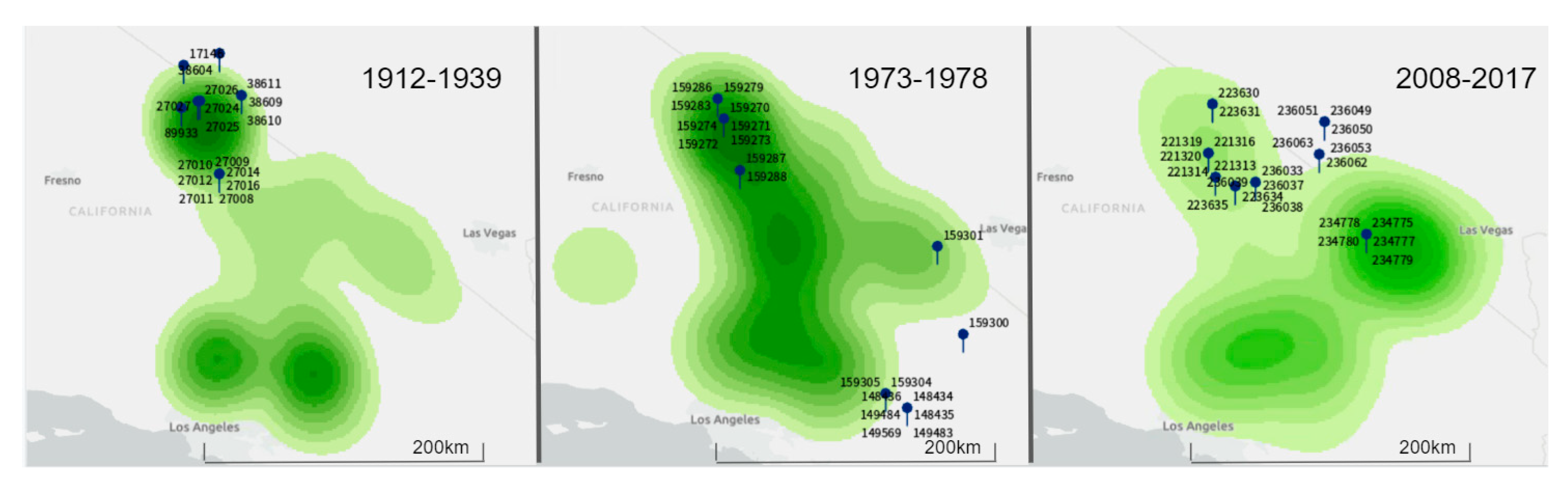
We used the VertNet database [23] of museum specimens to identify the geographic coordinates of D. microps collection sites on record for major museums across the USA. Most of these specimens were from Inyo County, California, USA and the surrounding area. We selected individual samples across three time periods. These were created to reflect the historic (1912–1939), intermediate (1973–1979) and the most recent (hereon ‘current’) samples (2008–2017) over the past century.

To identify areas with different saltbush abundances (specifically: Atriplex confertifolia) in south-eastern California, USA, we used the Global Biodiversity Information Facility (GBIF) website [24]. Because of the dramatic shift in land use over this time, both general disturbance and rangeland expansion were assumed to increase with time [25] which we expected to impact density of saltbush. The GBIF houses spatially referenced data. We downloaded all occurrences of saltbush in Inyo county, California, USA and the immediately surrounding area from 1868–2017 to take spatial distribution of saltbush and saltbush density (a proxy for distribution) over time into account when selecting individual D. microps to sample.

These data were collated using ArcGIS Pro (ESRI) and paired with collection site coordinates of D. microps. A series of maps were created illustrating kernel densities of saltbush as a proxy for local saltbush abundance. We generated three such maps (Figure 1) each reflecting local abundance of saltbush during one of the three time periods described above. The resulting maps were used to assign categories of low or medium-high saltbush abundance to the collection sites of individual D. microps georeferenced in VertNet. As a result, we were able to minimize biases in our sampling relative to saltbush abundance and ensure that D. microps individuals were sampled with similar representation from areas of differing local saltbush abundances in our final dataset. These maps were rendered by ArcGIS Pro 2.2.1 using the geoprocessing spatial analyst tool ‘kernel density.’ Point counts reported in decimal degrees were ranked into 10 classes using the geometric interval method available in ArcGIS Pro 2.2.1. However, we were unable to standardize density metrics of saltbush across different time periods because of differential surveying/sampling efforts. Thus, the abundance classifications in each map (Figure 1) are relative only to the baseline density within that time period. For this reason, these maps were used only for specimen selection and the classification of saltbush was not a factor in final analysis. Finally, seasonality during the time of collection was categorized based on temperature and precipitation using weather data from the National Oceanic and Atmospheric Association (NOAA) [26] from Inyo County, California, USA and categorized as either a warm (May-September) or cold (October–April) season.

Permission to collect hair samples from D. microps specimens was obtained from the Museum of Vertebrate Zoology (MVZ), University of California, Berkeley, California, USA. We selected individual specimens from the MVZ that reflected even representation by sex from each time period (final sample size N = 66). Finally, the extensive field notes of Dr. James L. Patton (Emeritus Professor, University of California, Berkeley) were used to identify a subset of specimens (N = 17) collected from trapping transects in 2017 from areas of high saltbush abundance (saltbush <40% of plants in the area; N = 4), medium abundance (<40% of foliage in the area identified as saltbush; N = 6), or in very low abundance to near absence (<5% of the plant cover in the immediate area; N = 7).

2.2. Hair Collection, Cleaning, and Preparation

Hair samples were obtained from museum skins housed at the MVZ. Approximately 2 g of hair was collected from the caudal region of the dorsum just above the tail and stored in 2 mL Eppendorf tubes until processed further. To prepare samples for stable isotope analyses, hair was cleaned with a 2:1 chloroform:methanol solution. Each sample was placed in a glass beaker and filled with enough solution to entirely cover the hair, and beakers were placed on a shaker plate set on low for 10 min. After shaking, the solution was drained from the beaker using filter paper to collect the hair. To ensure removal of excess dirt and oil that may change carbon signatures, these steps were repeated a total of three times. Once cleaned, the remaining solution was allowed to evaporate under a fume hood overnight. Dried hair samples were stored in 2 mL Eppendorf tubes prior to stable isotope analysis.

2.3. Sample Preparation for Stable Isotope Analysis

Approximately 0.75 g (±10%) of hair was weighed to the nearest 0.0001 g, recorded, and placed into tin capsules (Costech). Hairs were left intact and not ground into a powder as is the traditional method for processing hair samples (e.g., human hair) because the low density of the hair caused it to disperse in powder form.

Carbon (δ¹³C) and nitrogen (δ¹⁵N) values were measured with a continuous-flow mass spectrometer (Thermo Finnigan Delta Plus XL and a Carlo Erba CHN EA1110 elemental analyzer) at the University of Utah’s Stable Isotope Ratio Facility for Environmental Research (SIRFER). Isotope values were reported using delta (δ) notation in parts per mil (‰) as:

Δ‰ = (R_sample/R_standard) × 1000.

(1)

In the formula here, δ indicates the relative ratios of the heavy to light isotopes (¹³C/¹²C or ¹⁵N/¹⁴N) in a sample and standard, respectively. The standard reference material for carbon was Vienna Pee-Dee Belemnite (VPDB) with internal reference materials of glutamic acid and bovine muscle. Instrumental standard errors for the in-house standards relative to carbon were δ¹³C −25.2 ±0.2‰ VPDB, and δ¹³C –28.2 ± 0.1‰ VPDB, respectively. The same internal reference materials were used for nitrogen with standard errors of glutamic acid (δ¹⁵N 8.9 ± 0.1‰ AIR (atmospheric air)) and bovine muscle (δ¹⁵N 7.1 ± <0.01‰ AIR). These in-house standards were used to normalize our isotopic results to VPDB and AIR international standards.

2.4. Seuss Effect Correction of Carbon Values

Because δ¹³C values in atmospheric CO₂ have changed through the combustion of fossil fuels, we adjusted our δ¹³C values for hair. This pattern is termed the ‘Seuss effect’ or the ‘industrial δ¹³C effect’ [27] and has resulted in global shifts in atmospheric δ¹³C due to the use of fossil fuels over the last 150 years [28,29]. The magnitude of these changes in atmospheric δ¹³C is well documented, for example in ice cores [29,30]. We used these known changes to determine a correction factor to our measured δ¹³C values. All δ¹³C values prior to 1960 were adjusted by a value of −0.005‰ per year prior to 1960 and those after 1960 had a per year correction of 0.022‰ [30].

2.5. Baysian Mixing-Models to Estimate Saltbush Use

We used isotopic mixing models to estimate the proportion of an individual’s assimilated carbon that was derived from C₄ plants versus C₃ plants. All C₄ values are assumed to largely reflect saltbush because other C₄ plants are uncommon in these environments. To assess this representation, we used mixing models in the Stable Isotope Analysis in R (SIAR) package (v.4.2, 31). Specifically, we used the Stable Isotope Mixing Models in R (SIMMR) package which is an updated version of the commonly used Bayesian SIAR mixing model [31]. This package was run in R (v.3.5.2, R Development Core Team 2015). We chose this package so as to make our results comparable with those of Terry et al. [14], who used SIAR in their analysis. However, since we were considering the contributions of only three dietary sources, C3 plants, C4 plants, and insects to the diet of a single species.

For our SIAR mixing models, all of our plant values for both δ¹³C and δ¹⁵N were derived from a previous study looking at other Dipodomys species [14]. Although these values were unavailable from the exact location of our museum samples, they are from the same ecosystem and should encapsulate the ranges seen for plants at our sites. These plant δ¹³C and δ¹⁵N values as well as their standard deviations (listed below) were included for these two possible plant food sources in SIAR [31]. Saltbush values resemble those of other C₄ plants, δ¹³C = −14.1 ± 0.9‰ [10,14] whereas C₃ plants have values around δ¹³C = −24.5 ± 1.9 ‰ VPDB. Values for C₄ plants were δ¹⁵N = 8.6 ± 1.2‰ [14], whereas C₃ plants have values around δ¹⁵N = 5.5 ± 1.6‰ AIR [14]. The Bayesian mixing model analysis included the application of 30,000 Markov simulations to create probability distributions for both C₃ and C₄ plants [31].

Diet-to-tissue fractionation values are included in diet analyses to reflect the physiological processes of an animal that alter how isotope ratios are conserved in the body. Namely, the raw value of carbon/nitrogen isotopes in food items will not be the exact same values in body tissues due to these processes [18,32]. Our carbon diet-to-tissue fractionation value (∆¹³C_{diet to hair}) was input into the models as α = 2.0‰, which was an average of other similar studies on herbivorous mammals because this value has not been experimentally determined for the species herein [33,34,35]. Our nitrogen diet-to-tissue fractionation value (∆¹⁵N_{diet to hair}) was included in our models and estimated to be α = 3.2 ‰ [14,19,20,34,35]. The three independent variables in our three SIAR models were 1) time period (historic, intermediate, current); 2) season of collection (warm, cold); and 3) density of salt bush (very low, medium, high) in a subset of samples all from the same time (2017) to prevent confounding the effect of year and differences in estimates of saltbush abundance. We examined insects as an additional possible food source. To do so we used the isotope values reported by Terry et al. [14]. The δ¹³C value for insects in our models was −22.877 ± 0.74‰ and the δ¹⁵N value 10.339 ± 3.54‰. For all of our analyses, SIMMR provided group comparisons with p-values for each categorical variable (post-hoc tests). We report this in our figures below as ‘significant’ if p < 0.013.

2.6. Analysis using Mixing Model

To further evaluate diet, the percent of C₄ plants in the diet was also calculated using a two-point mixing-model based on the same plant values described above for SIAR, where p is the percent of C₄ plants in the diet [14,32]. This enabled an individual assignment of percent saltbush in the diet that we were able to analyze in SPSS (v25) (

Table 1. Information for individual specimens from the Museum of Vertebrate Zoology (MVZ) at the University of California, Berkeley, California, USA. Data are listed by MVZ catalog number for each specimen sampled (which can be compared to Figure 1 for locations). Corresponding data on δ¹³C‰ and δ¹⁵N‰ are reported for each sample together with δ¹³C‰ values after they were corrected for atmospheric carbon changes from the Seuss effect. Percent saltbush was calculated using a two-point mixing model and should be interpreted separately from the Baysian SIAR mixing-model outputs (Figure 2, Figure 3, Figure 4 and Figure 5), but is included here to provide readers a general estimate of percentage saltbush on a per-individual basis.

MVZ Catalog Number	Month	Season	Year	δ15N‰ AIR	δ13C‰ VDPB	Seuss Adjusted δ13C‰ VDPB	Percent Saltbush
17146	July	Warm	1912	15.54	−16.91	−17.15	51.45
27009	June	Warm	1917	15.46	−17.73	−17.82	45.01
27016	June	Warm	1917	15.86	−17.75	−17.83	44.86
27010	June	Warm	1917	15.67	−15.01	−15.10	71.16
27008	June	Warm	1917	15.93	−18.61	−18.69	36.63
27012	June	Warm	1917	16.10	−14.50	−14.58	76.11
27011	June	Warm	1917	17.01	−16.92	−17.00	52.85
27013	June	Warm	1917	15.69	−16.15	−16.23	60.27
27014	June	Warm	1917	17.08	−17.43	−17.51	47.97
27017	June	Warm	1917	14.35	−14.79	−14.88	73.30
27015	June	Warm	1917	16.60	−14.57	−14.66	75.39
27024	August	Warm	1917	12.15	−16.41	−16.49	57.79
27025	August	Warm	1917	11.84	−16.39	−16.48	57.89
27026	August	Warm	1917	11.93	−16.53	−16.62	56.56
27027	August	Warm	1917	9.91	−16.46	−16.54	57.28
38604	May	Warm	1927	13.45	−19.10	−19.27	31.09
38611	June	Warm	1927	13.48	−20.27	−20.43	19.87
38609	June	Warm	1927	12.40	−15.48	−15.64	65.96
38610	June	Warm	1927	13.48	−16.28	−16.45	58.18
89933	December	Cold	1939	10.07	−20.86	−21.02	14.19
159301	April	Cold	1973	7.68	−16.27	−15.99	62.64
159271	November	Cold	1973	15.53	−16.54	−16.26	60.03
159274	November	Cold	1973	15.93	−16.83	−16.55	57.25
149569	October	Cold	1975	4.62	−21.04	−20.71	17.22
148434	March	Cold	1975	3.36	−22.11	−21.78	6.97
148435	March	Cold	1975	3.51	−20.99	−20.66	17.67
148436	March	Cold	1975	2.22	−21.26	−20.93	15.13
149483	October	Cold	1975	4.87	−20.44	−20.11	22.97
149484	October	Cold	1975	4.32	−21.34	−21.01	14.30
159304	September	Warm	1976	3.45	−19.82	−19.47	29.16
159305	March	Cold	1976	3.69	−22.01	−21.66	8.12
159287	May	Warm	1976	13.94	−16.97	−16.62	56.54
159283	August	Warm	1976	11.45	−15.87	−15.52	67.16
159288	May	Warm	1976	15.03	−15.01	−14.66	75.37
159270	August	Warm	1976	13.24	−18.57	−18.22	41.14
159279	August	Warm	1976	11.32	−14.59	−14.23	79.48
159286	August	Warm	1976	11.27	−14.78	−14.43	77.59
159300	May	Warm	1978	3.62	−19.70	−19.31	30.68
159272	Mar	Cold	1978	15.50	−18.04	−17.65	46.67
159273	May	Warm	1978	8.49	−17.30	−16.90	53.82
221314	April	Cold	2008	10.33	−18.98	−17.92	44.03
221320	May	Warm	2008	8.26	−18.04	−16.99	53.01
221313	April	Cold	2008	13.89	−18.11	−17.05	52.38
221319	May	Warm	2008	10.10	−15.72	−14.67	75.33
221316	May	Warm	2008	9.45	−22.02	−20.97	14.73
223634	April	Cold	2009	12.75	−17.02	−15.94	63.05
223635	May	Warm	2009	14.47	−15.39	−14.31	78.73
223631	May	Warm	2009	11.37	−14.23	−13.15	89.93
223630	May	Warm	2009	12.42	−18.32	−17.24	50.60
236049	October	Cold	2017	7.98	−17.04	−15.78	64.57
236050	October	Cold	2017	11.20	−21.32	−20.07	23.40
236051	October	Cold	2017	12.83	−20.74	−19.49	28.95
236053	October	Cold	2017	8.06	−18.28	−17.03	52.62
234780	March	Cold	2017	6.79	−21.38	−20.12	22.86
234777	March	Cold	2017	7.20	−22.65	−21.40	10.62
234775	March	Cold	2017	5.45	−22.43	−21.18	12.70
234778	March	Cold	2017	7.23	−21.15	−19.89	25.07
234779	March	Cold	2017	5.96	−21.33	−20.07	23.32
236062	October	Cold	2017	6.84	−22.25	−21.00	14.43
236063	October	Cold	2017	7.35	−23.51	−22.25	2.36
236039	September	Warm	2017	11.79	−19.17	−17.92	44.04
236040	September	Warm	2017	10.84	−19.93	−18.68	36.76
236038	September	Warm	2017	9.33	−20.24	−18.99	33.76
236041	September	Warm	2017	10.60	−20.08	−18.82	35.34
236037	September	Warm	2017	11.97	−18.55	−17.30	50.02
236033	September	Warm	2017	10.91	−18.01	−16.76	55.23

).

δ¹³C_(tissue) = p(δ¹³C(C₄)) + (1 − p)(δ¹³C(C₃)) + α

(2)

This allowed us the option to use Analysis of Variance (ANOVAs) for each of our independent variables to confirm if the percent of incorporated carbon indicative of animals ingesting C₄ plants varied for each of our predictor variables as indicated by SIAR. When appropriate, ANOVAs were followed by post-hoc Fisher’s Least Significant Difference (LSD) tests to look at differences between categories (ex. time periods) (Figure 2, Figure 3, Figure 4 and Figure 5). We focus our interpretation of saltbush percentages on SIAR results below unless otherwise noted. In cases of conflicting results between ANOVA and SIAR results, we focused our interpretations on the SIAR results as these include both carbon and nitrogen data, and are generally preferred to two-point mixing models [14,31].

3. Results

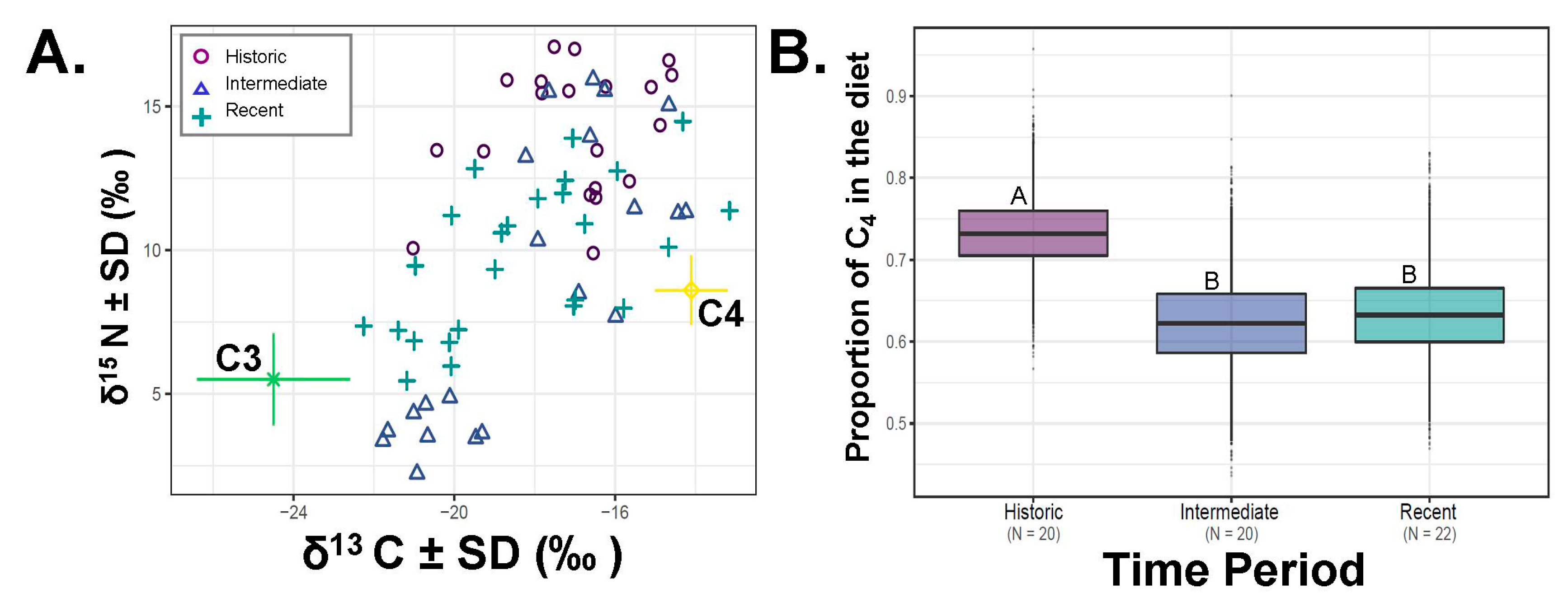
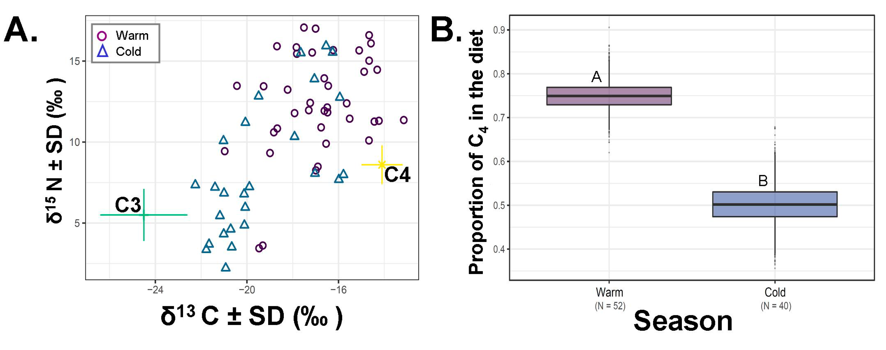
The average estimated consumption of saltbush across all D. microps samples in our data set was 66.3% (SE = ± 0.01, N = 66; 64.8–73.5%; Figure 2). Time-period and season impacted the variation in saltbush consumption when considered by SIAR (Figure 2, Figure 3). Time-period was not different when considered in an ANOVA based only on the two-point mixing model (F _2,65 =1.942, p = 0.152, all post-hoc tests p > 0.199). Over the past century, the ingestion of saltbush declined in our samples relative to historic samples (Figure 2, SIAR p < 0.008). Individuals from the historic, intermediate and current time periods averaged 73.3% ± 0.01%, 62.2% ± 0.01%, 63.4% ± 0.01% saltbush ingestion, respectively. Diet also varied by season (ANOVA F_1,65 = 29.69, p < 0.001) with respect to the estimates of saltbush consumption, where the warm season averaged 74.9% (N = 52, SE = ± 0.00%) and the cold season averaged 50% saltbush (N = 40, SE = ± 0.01%; Figure 3).

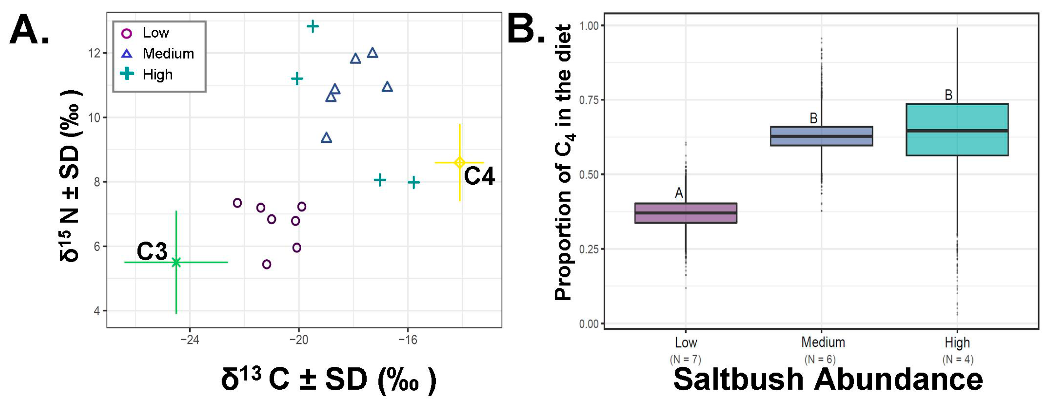
In the recent samples from 2017, saltbush consumption was related with its relative abundance (Figure 4). Animals collected from areas where saltbush was very low in abundance differed from all other groups (ANOVA F_2,16=10.52, p = 0.002, SIAR Figure 4B). The percentage of dietary saltbush estimated for individuals collected in areas with very low documented saltbush was 36.9 ± 0.02% (N = 7, minimum = 27.1%, maximum = 46.5% dietary saltbush). The consumption of saltbush from individuals collected in areas of medium abundance of saltbush averaged 62.4 ± 0.02 % (N = 6, minimum = 52.2%, maximum = 74.9%). In areas with high abundance of saltbush, the percentage of dietary saltbush averaged 64.3 ± 0.07% (N = 4, minimum = 33.1%, maximum = 91.7%; Figure 4). Individual attributes, raw values and percent of C₄ consumption are detailed in Table 1.

Our results for models that included insects as a possible source revealed substantial reliance on this food source (around 26% of the diet; Figure 5). Indeed, once insects were included in our SIAR models, time period was a clear predictor of saltbush ingestion (SIAR p < 0.008; Figure 5).

4. Discussion

The primary aim of this study was to determine if D. microps is an obligate dietary specialist on saltbush (Atriplex spp.). The three criteria for a dietary specialization proposed by Shipley et al. [4]—difficult diet, morphological use relative to availability, and relatively high abundance of the particular food item—were not fully met in our study. Dipodomys microps does ingest a difficult diet, i.e., plant with saline wax, and it has morphological adaptations to deal with the challenges of this food item, i.e., specialized incisors. Although we did not have quantitative measures for saltbush availability to compare to intake, a qualitative assessment suggests that D. microps did not seem to use saltbush to a greater extent in areas with relatively higher saltbush abundances (relative to other foods) (Figure 4). Our categorical assignments of saltbush abundances do not provide extensive resolution on the exact proportion of saltbush in the area and how this relates to its proportion in the diets of D. microps, but this would be an exciting future avenue. Our work differs from another recent study that found that saltbush rarely constituted 60% of the diet of D. microps [14]. The majority of the animals in our study consumed more than 60% saltbush, although there were some individuals consuming less saltbush (Figure 2, Figure 3). In cases when at least 60% of an individual’s diet constituted a single food item we considered them a dietary specialist [1]. Moreover, insects represented a quarter of the diet (Figure 5). Taken together, these results suggest that while D. microps has some specializations for feeding on saltbush (e.g., unusual incisors and feeding behaviors), it is a facultative specialist of saltbush. We elaborate on evidence for this conclusion below relative to our findings.

We qualitatively tested whether saltbush ingestion differed with the relative abundance of saltbush (Figure 4). This particular avenue is unique relative to the earlier study by Terry et al. [14]. Dietary ingestion of saltbush by D. microps was related to its local abundance to some extent in our findings, although these findings are based on categorical assignments of saltbush abundance. We found that in areas of very low saltbush abundance (none to very little saltbush noted in the area), roughly one third of the diet still originated from saltbush. This finding suggests that D. microps is seeking this plant out across the landscape. However, when saltbush was more available i.e., in areas with intermediate (40% or less) and high abundance (40% or more), ingestion increased but plateaued even with high saltbush abundance, and only in 10% of all individuals did its ingestion ever exceed 60%. These results indicate that D. microps does not require a high level of saltbush, and when saltbush is abundantly available, it does not choose to ingest a diet exclusively of saltbush. These results are consistent with the category of facultative specialist [4].

We also tested whether there was a directional diet shift over time in D. microps individuals from the same general area (Inyo County, California, USA) over the past century (1912–2017). We saw a dramatic decrease in overall consumption of saltbush from historical samples taken in 1912–1939 to more current values: 2008–2017. Specifically, we documented a 50% reduction in the amount of saltbush ingested by D. microps today versus a century ago. In turn, we take this as further support for dietary plasticity within this species. Furthermore, our observations align with observations of niche flexibility noted by other studies spanning samples from prehistoric conditions through today [14].

Dietary flexibility was also noted seasonally, whereby individuals seem to eat more saltbush in the warmer part of the year relative to the cooler part of the year (Figure 3). We suggest that saltbush may provide an important source of water during the hotter portion of the year. These data would be consistent with this finding, such that individuals may shift to eating saltbush during part of the year when water demands are high and can be met through saltbush ingestion. However, another explanation for this observation is that plants exhibit bias in δ¹³C isotopes during different times of the year (due to heat challenges) [36,37]. For this reason, we cannot be entirely certain that the higher isotope signal during the warm season is due to a more saltbush-rich diet.

Our results are somewhat similar to those from a recent study [14] that focused on the prehistoric diets of D. microps using fossils from owl nests from a single location in Washoe County, Nevada. However, in that study, D. microps ingested less saltbush overall compared to our findings from Inyo County, California. This suggests D. microps has a broad tolerance to the variation in abundance of saltbush in its environment, and it may be plastic in its degree of specialization on this plant.

Considering our findings and those of others [5,14,15,16], why was D. microps classified as an exemplary obligate specialist in the first place? Early studies of this species relied on observations made in the laboratory [5,8,12]. Such studies controlled the environment in ways that eliminated many pressures realized in nature, such as water-limitation, a broader range of alternative plants available to ingest, and the energetic costs of foraging [38]. For example, in one experiment, D. microps individuals were given access exclusively to saltbush, while others were given access to limited saltbush leaves and ad lib sunflower seeds, and a final group was given access to birdseed with no water (a diet that would be feasible for some species of Dipodomys but D. microps died [5,8]). Thus, the results of laboratory studies coupled with the discovery of teeth morphologically specialized for eating saltbush leaves suggested a high level of dietary specialization.

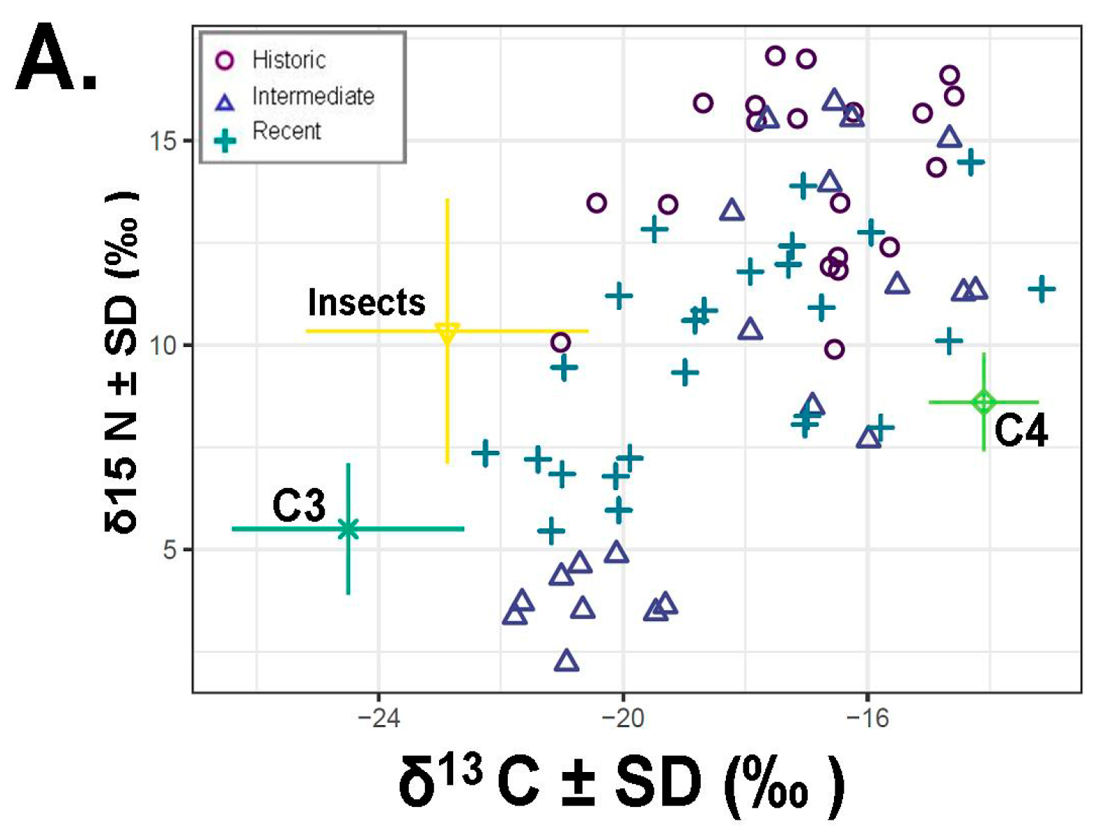
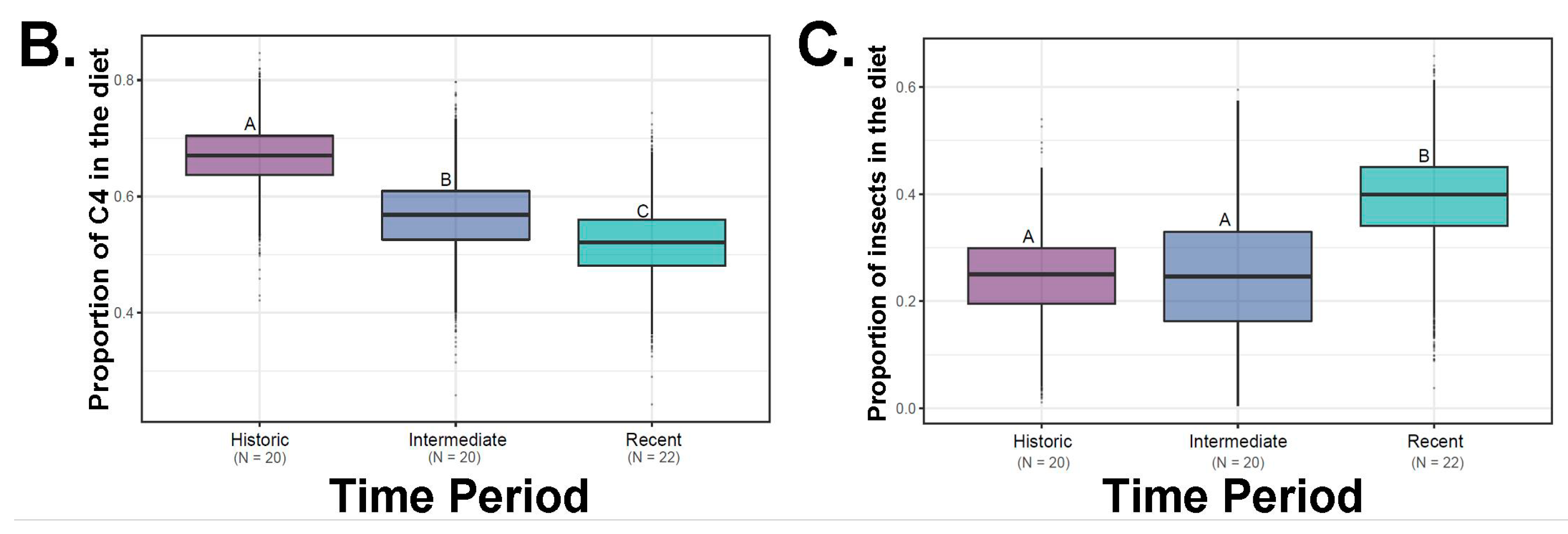
Several previous studies reported that D. microps also consumes insects [6,14]. Indeed, the analysis of the d¹⁵N values in this dataset are consistent with the ingestion of significant quantities of insects (Figure 5, Table 1). Furthermore, insectivory seems to be common as evidenced by the isotope signature for the consumption of insects across numerous individuals (Figure 5). There is also evidence of alterations between food items, such that when insects are common in the diet, less saltbush is ingested (Figure 5). It is possible that both of these food sources provide critical water resources when present and that insects provide high levels of protein not found in a diet of saltbush.

Another potential component in the diet of D. microps is blackbush (Coleogyne ramosissima), a C₃ shrub, which occurs in vegetation zones where saltbush abundance is low but D. microps are present [8]. The ability of D. microps to incorporate these and other food items into its diet may explain why it has been able to persist over time in areas with low saltbush abundances. This is especially relevant under changing environmental pressures such as rangeland expansion (and associated changes in the plant community), the introduction of invasive species, and increased annual temperatures that alter plant communities [36]. Based on these studies and our own observations, we suggest that while D. microps can survive on saltbush alone in the laboratory [5,8], under natural conditions, it clearly also incorporates other food items.

Facultative specialization of D. microps may allow it to behaviorally respond to changing environmental conditions by incorporating new foods in its diet. Invasive cheatgrass (Bromus tectorum) has altered many plant communities in the Great Basin [37,39], and monthly temperatures and aridity have increased over the past century, which can decrease saltbush productivity [36,37,40]. These changes may have caused the dietary reduction in saltbush by D. microps found in this time frame (Figure 2).

Dietary specialization is not only interesting from an evolutionary and ecological perspective but also relative to species conservation. Indeed, specialization places a species more at risk of extinction or population decrease because of a fixed requirement for certain foods that may decrease in abundance [41]. As a consequence, specialists tend to decline as availability of their food source decreases [4]. Facultative specialists and generalists, however, are capable of responding to these same pressures by incorporating alternative foods in their diet [4,41]. In regards to conservation, accurately categorizing animals as obligate specialists, facultative specialists or generalists may well inform us about conservation risk and also highlights the importance of whole-ecosystem mitigation efforts.

References

- Dearing, M.D.; Mangione, A.M.; Karasov, W.H. Diet breadth of mammalian herbivores: Nutrient versus detoxification constraints. Oecologia 2000, 123, 397–405. [Google Scholar] [CrossRef] [PubMed]
- Westoby, M. What are the biological bases of varied diets? Am. Nat. 1978, 112, 627–631. [Google Scholar] [CrossRef]
- Freeland, W.J.; Janzen, D.H. Strategies in herbivory by mammals: The role of plant secondary compounds. Am. Nat. 1974, 108, 269–289. [Google Scholar] [CrossRef]
- Shipley, L.A.; Forbey, J.S.; Moore, B.D. Revisiting the dietary niche: When is a mammalian herbivore a specialist? Int. Comp. Biol. 2009, 49, 274–290. [Google Scholar] [CrossRef] [PubMed] [Green Version]
- Kenagy, G.J. Adaptations for leaf eating in the Great Basin kangaroo rat, Dipodomys microps. Oecologia 1973, 12, 383–412. [Google Scholar] [CrossRef] [PubMed]
- Hayssen, V. Dipodomys microps. Mamm. Species 1991, 389, 1–9. [Google Scholar] [CrossRef]
- Breyen, L.J.; Bradley, W.G.; Yousef, M.K. Physiological and ecological studies on the chisel-toothed kangaroo rat, Dipodomys microps. Comp. Biochem. Phys. Part A Phys. 1973, 44, 543–555. [Google Scholar] [CrossRef]
- Csuti, B. Patterns of adaptation and variation in the Great Basin kangaroo rat. Univ. Calif. Publ. Zool. 1979, 111, 1–69. [Google Scholar]
- Walsberg, G.E. Small mammals in hot deserts: Some generalizations revisited. AIBS Bull. 2000, 50, 109–120. [Google Scholar] [CrossRef]
- Sandquist, D.R.; Ehleringer, J.R. Carbon isotope discrimination in the C4 shrub Atriplex confertifolia along a salinity gradient. Great Basin Nat. 1995, 55, 135–141. [Google Scholar]
- Mares, M.A.; Ojeda, R.A.; Borghi, C.E.; Giannoni, S.M. How desert rodents overcome halophytic plant defenses. BioScience 1997, 47, 699–704. [Google Scholar] [CrossRef]
- Jacobs, J.F.; Koper, G.J.M.; Ursem, W.N.J. UV protective coatings: A botanical approach. Prog. Org. Coat. 2007, 58, 166–171. [Google Scholar] [CrossRef]
- Kenagy, G.J. Saltbush leaves: Excision of hypersaline tissue by a kangaroo rat. Science 1972, 178, 1094–1096. [Google Scholar] [CrossRef] [PubMed]
- Terry, R.C.; Guerre, M.E.; Taylor, D.S. How specialized is a diet specialist? Niche flexibility and local persistence through time of the Chisel-toothed kangaroo rat. Funct. Ecol. 2017, 31, 1921–1932. [Google Scholar] [CrossRef]
- Jezkova, T.; Olah-Hemmings, V.; Riddle, B.R. Niche shifting in response to warming climate after the last glacial maximum: Inference from genetic data and niche assessments in the chisel-toothed kangaroo rat (Dipodomys microps). Glob. Chang. Biol. 2011, 17, 3486–3502. [Google Scholar] [CrossRef]
- Riddle, B.R.; Jezkova, T.; Hornsby, A.D.; Matocq, M.D. Assembling the modern Great Basin mammal biota: Insights from molecular biogeography and the fossil record. J. Mammal. 2014, 95, 1107–1127. [Google Scholar] [CrossRef]
- Tieszen, L.L.; Buotton, T.W.; Tesdahl, K.G.; Slade, N.A. Fractionation and turnover of stable carbon isotopes in animal tissues: Implications for δ13C analysis of diet. Oecologia 1983, 57, 32–37. [Google Scholar] [CrossRef] [PubMed]
- Post, D.M. Using stable isotopes to estimate trophic position: Models, methods, and assumptions. Ecology 2002, 83, 703–718. [Google Scholar] [CrossRef]
- Hobson, K.A. Stable isotope analysis of marbled murrelets: Evidence for freshwater feeding and determination of trophic level. Condor 1990, 92, 897–903. [Google Scholar] [CrossRef]
- Orr, T.J.; Ortega, J.; Medellín, R.A.; Sánchez, C.D.; Hammond, K.A. Diet choice in frugivorous bats: Gourmets or operational pragmatists? J. Mammal. 2016, 97, 1578–1588. [Google Scholar] [CrossRef]
- Wang, L.; D’Odorico, P.; Ries, L.; Macko, S.A. Patterns and implications of plant-soil δ13C and δ15N values in African savanna ecosystems. Q. Res. 2010, 73, 77–83. [Google Scholar] [CrossRef]
- Aranibar, J.N.; Anderson, I.C.; Epstein, H.E.; Feral, C.J.W.; Swap, R.J.; Ramontsho, J.; Macko, S.A. Nitrogen isotope composition of soils, C3 and C4 plants along land use gradients in southern Africa. J. Arid Environ. 2008, 72, 326–337. [Google Scholar] [CrossRef]
- VertNet. Available online: http://vertnet.org/ (accessed on 1 September 2016).
- Global Biodiversity Information Facility (GBIF). Available online: https://www.gbif.org (accessed on 1 September 2016).
- Rowe, R.J.; Terry, R.C.; Rickart, E.A. Environmental change and declining resource availability for small-mammal communities in the Great Basin. Ecology 2011, 92, 1366–1375. [Google Scholar] [CrossRef] [PubMed]
- National Oceanic and Atmospheric Association (NOAA). Available online: https://www.noaa.gov (accessed on 15 April 2017).
- McCarroll, D.; Gagen, M.H.; Loader, N.J.; Robertson, I.; Anchukaitis, K.J.; Los, S.; Young, G.H.; Jalkanen, R.; Kirchhefer, A.; Waterhouse, J.S. Correction of tree ring stable carbon isotope chronologies for changes in the carbon dioxide content of the atmosphere. Geochim. Cosmochim. Acta 2009, 73, 1539–1547. [Google Scholar] [CrossRef]
- Al-Rousan, S.; Pätzold, J.; Al-Moghrabi, S.; Wefer, G. Invasion of anthropogenic CO2 recorded in planktonic foraminifera from the northern Gulf of Aqaba. Int. J. Earth Sci. 2004, 93, 1066–1076. [Google Scholar] [CrossRef]
- Keeling, R.F.; Graven, H.D.; Welp, L.R.; Resplandy, L.; Bi, J.; Piper, S.C.; Sun, Y.; Bollenbacher, H.A. Atmospheric evidence for a global secular increase in carbon isotopic discrimination of land photosynthesis. Proc. Natl. Acad. Sci. USA 2017, 114, 10361–10366. [Google Scholar] [CrossRef] [PubMed] [Green Version]
- Francey, R.J.; Frederiksen, J.S. The 2009–2010 step in atmospheric CO2 interhemispheric difference. Biogeosciences 2016, 13, 873–885. [Google Scholar] [CrossRef]
- Parnell, A.C.; Inger, R.; Bearhop, S.; Jackson, A.L. Source partitioning using stable isotopes: Coping with too much variation (ed. SRands). PLoS ONE 2010, 5, e9672. [Google Scholar] [CrossRef]
- Orr, T.J.; Newsome, S.D.; Wolf, B.O. Cacti supply limited nutrients to a desert rodent community. Oecologia 2015, 178, 1045–1062. [Google Scholar] [CrossRef]
- Dalerum, F.; Angerbjörn, A. Resolving temporal variation in vertebrate diets using naturally occurring stable isotopes. Oecologia 2005, 144, 647–658. [Google Scholar] [CrossRef]
- Sponheimer, M.; Robinson, T.; Ayliffe, L.; Passey, B.; Roeder, B.; Shipley, L.; Lopez, E.; Cerling, T.; Dearing, D.; Ehleringer, J. An experimental study of carbon-isotope fractionation between diet, hair, and feces of mammalian herbivores. Can. J. Zool. 2003, 81, 871–876. [Google Scholar] [CrossRef]
- Sare, D.T.; Millar, J.S.; Longstaffe, F.J. Moulting patterns in Clethrionomys gapperi. Acta Theriol. 2005, 50, 561–569. [Google Scholar] [CrossRef]
- Naumburg, E.; Housman, D.C.; Huxman, T.E.; Charlet, T.N.; Loik, M.E.; Smith, S.D. Photosynthetic responses of Mojave Desert shrubs to free air CO2 enrichment are greatest during wet years. Glob. Chang. Biol. 2003, 9, 276–285. [Google Scholar] [CrossRef]
- Novak, S.J.; Mack, R.N. Tracing plant introduction and spread: Genetic evidence from Bromus tectorum (cheatgrass). BioScience 2001, 51, 114. [Google Scholar] [CrossRef]
- Pyke, G.H.; Pulliam, H.R.; Charnov, E.L. Optimal foraging: A selective review of theory and tests. Q. Rev. Biol. 1977, 52, 137–154. [Google Scholar] [CrossRef]
- Morris, L.R.; Rowe, R.J. Historical land use and altered habitats in the Great Basin. J. Mammal. 2014, 95, 1144–1156. [Google Scholar] [CrossRef] [Green Version]
- Mooney, H.A.; Gulmon, S.L. Environmental and Evolutionary Constraints on the Photosynthetic Characteristics of Higher Plants. In Topics in Plant Population Biology; Palgrave: London, UK, 1979; pp. 316–337. [Google Scholar]
- Kelly, P.M.; Adger, W.N. Theory and practice in assessing vulnerability to climate change and Facilitating adaptation. Clim. Chang. 2000, 47, 325–352. [Google Scholar] [CrossRef]
Figure 1.
Saltbush density maps for the study area in Inyo County, California, USA. Numbers surrounding pins indicate the catalog numbers of museum specimens (see Table 1 for additional information on each of these individuals). The color intensity on each map corresponds to saltbush density with darker colors indicating greater densities. Because the baseline densities and associated sampling are only relative to each time period, these maps are not intended to be compared across time-periods as sampling efforts cannot be standardized and likely differed between each period.
Figure 2.
Percent of C4 plants in Dipodomys microps’ diet for relative time periods. (A) Raw data for carbon (δ13C‰) and nitrogen (δ15N‰) values for each individual sample. Colored lines around food sources (C3, C4) are the associated standard deviations for the plant values in our analysis. (B) average saltbush consumption as estimated by our Stable Isotope Analysis in R (SIAR) mixing-models. Means are indicated by the horizontal line and for historic (1912–1939), intermediate (1973–1978), and current (2008–2017). The boxes above and below this line are the upper (Q3) and lower (Q2) quartiles and the whiskers the first (lower whisker, Q1) and last (upper whisker, Q4). Different letters indicate significant differences in SIAR.
Figure 3.
Percent of saltbush in Dipodomys microps’ diet across season (warm: May–September or cold: October–April). (A) Plot of the raw carbon (δ13C‰) and nitrogen (δ15N‰) data. Colored lines around food sources (C3, C4) are the associated standard deviations for the plant values in our analysis. (B) Boxplots from SIAR that represent the lower and upper quartiles around the mean relative to our data as pooled by season either warm or cool. Means are indicated by the horizontal line within boxes (Warm; 74.9% and Cold; 50.3%). The boxes above and below this line are the upper (Q3) and lower (Q2) quartiles and the whiskers the first (lower whisker, Q1) and last (upper whisker, Q4). Different letters indicate significant differences as indicated by an ANOVA.
Figure 4.
Percent of C4 plants in the diet of Dipodomys microps relative to saltbush abundance. (A) Raw carbon (δ13C‰) and nitrogen (δ15N‰) values for D. microps hair collected at sites with different saltbush abundance categories (low, medium, high). Colored lines around food sources (C3, C4) are the associated standard deviations for the plant values in our analysis. (B) Average saltbush consumption as calculated from our SIAR mixing-model. The boxes above and below this line are the upper (Q3) and lower (Q2) quartiles and the whiskers the first (lower whisker, Q1) and last (upper whisker, Q4). Different letters indicate significant differences from both SIAR and Fisher’s Least Significant Difference (LSD) post-hoc tests.
Figure 5.
(A) Plot showing the δ13C‰ and δ15N‰ values for three putative diet types: C3 and C4 (saltbush) plants as well as insects in our SIAR models plotted relative to year. Colored lines around food sources (C3, C4, insects) are the associated standard deviations for the plant and insect values used in our analysis. Boxplots from SIAR that represent the lower and upper quartiles around the mean horizontal line) relative to our data as pooled by (B) proportion of saltbush in the diet over time or (C) proportion of insects over time period. The boxes above and below this line are the upper (Q3) and lower (Q2) quartiles and the whiskers the first (lower whisker, Q1) and last (upper whisker, Q4). Different letters indicate significant differences from SIAR.