Forecasting Extinctions: Uncertainties and Limitations

Abstract

Extinction forecasting is one of the most important and challenging areas of conservation biology. Overestimates of extinction rates or the extinction risk of a particular species instigate accusations of hype and overblown conservation rhetoric. Conversely, underestimates may result in limited resources being allocated to other species/habitats perceived as being at greater risk. In this paper I review extinction models and identify the key sources of uncertainty for each. All reviewed methods which claim to estimate extinction probabilities have severe limitations, independent of if they are based on ecological theory or on rather subjective expert judgments.

1. Introduction

“Prediction is very difficult, especially about the future”

Nils Bohr, Nobel Prize winning physicist

Preventing the extinction of species is probably the most emblematic objective of the global conservation movement. To fulfill this aim effectively requires that decision makers and environmental managers are provided with accurate information on: (1) the identities of specific species/populations with a high probability of going extinct without further interventions; (2) the predicted rates of extinction among a range of taxa in different geographic areas and biomes under various ecological scenarios. Armed with this information rational decisions can then be made on the allocation of resources to habitat or species protection measures with the aim of reducing the likelihood of a species going extinct or a reduction in the general rate of extinctions over a wider area.

Although the rationale for accurate assessment of extinction risk for a species or a geographic area is clear, the best techniques for achieving these objectives have not been resolved. Indeed, extinction forecasting is one of the most problematic and controversial areas of conservation science where crude estimates (e.g., [1]) have been the subject of high profile criticism by environmental skeptics [2] or have become the subject of misleading newspaper headlines [3]. The uncertainty surrounding extinction forecasting is understandable given the diversity of available methods, each of which is based on various assumptions and all of which use a wide variety of data or varying quality and completeness. In this short review article I create a simple typology for defining different classes of extinction forecasting models and to identify the key assumptions and sources of uncertainty for each category of model. I will conclude with a discussion on the role of human agency in avoiding extinction and argue that, ultimately, it is the reaction of the global conservation movement to information on extinction risk that determines the probability of extinction for many taxa and that this should be factored into future extinction models. This review is aimed at conservation scientists, researchers and especially the growing numbers of interdisciplinary academics who are in the process of incorporating ideas from social science and practice into the standard natural science framework used in conservation.

Before presenting the typology of extinction models it is important to consider what is meant by extinction. Extinction has traditionally been viewed by conservation scientists as logical end point of the process of population decline—the point on the graph where the population size curve meets the x-axis and terminates abruptly and finally [4]. The IUCN defines a species as extinct if “there is no reasonable doubt that the last individual has died” [5], a definition that reveals one of the main stumbling blocks for measuring extinction: the difficulty of ascertaining the continued existence of a species that is certainly exceedingly rare, and which may also inhabit an isolated habitat that is difficult to effectively survey. Indeed, IUCN guidelines require that a species can be declared extinct only after exhaustive surveys fail to produce any observations over an appropriate time period and geographical range appropriate to its life cycle and life-form—an unfeasible task for most species [6]. Butchart and his colleagues have recently introduced a new category of ‘possibly extinct’ to apply to those species that are, “on the balance of evidence, likely to be extinct, but for which there is a small chance that they may be extant and thus should not be listed as ‘Extinct’ until adequate surveys have failed to find the species and local or unconfirmed reports have been discounted” [7].

The above definitions are concerned with situations where a species is known to science and has been collected (on at least one occasion). However, if science was to restrict extinction forecasts only to those species that have been formally identified there would be a danger of considerable underestimations in magnitude. Extinctions of undiscovered species inferred from estimates of species diversity for a given ecosystem or region and the species-area relationship have been termed Linnean extinctions [4] (after the Linnean shortfall in biogeography) or Centinelan extinctions [8] and probably outnumber documented extinctions many times over. Such unseen extinctions are highly dependent of estimates of species richness and are the source of most of the headline grabbing figures that periodically appear in the global press. Moreover, the majority of such extinctions are in poorly described taxa and biomes such as arthropods in tropical forests.

2. A Typology of Extinction Forecasting

Extinction forecasting models are defined here as any model/method that indicates: (i) the likelihood that a species is already extinct, or will go extinct at some defined point in the future; (ii) the number of species that are likely to go extinct within a given geographic area within a given timeframe. In this respect extinction forecasting can answer 4 key questions for conservationists (Table 1):

• How many species are likely to go extinct in area x over time t?
• What are the identities of the species with a high probability of extinction in area x over time t?
• What is the probability of species y going extinct in habitat x over time t?
• What is the probability that species y is already extinct in habitat x?

Table 1. A use-based framework for classifying extinction forecasting models based on the four fundamental questions about extinction (see text for full explanation). Model choice is critically constrained by type of data available. Specificity refers to taxonomic level (individual species versus extinctions within a defined area) and geographical focus.

Specificity	Key Question	Data available	Models
General	How many species will go extinct in area x over time t?	Estimates of species richness/endemism Estimates of habitat loss	Species-area relationshipNeutral theory
		Environment-species richness correlations Extinction rate estimates	Extrapolation Simple deterministic relationships
	What are the identities of the species with a high probability of extinction in area x over time t?	Species inventory Biogeographic data (e.g., distribution, dispersal, etc.) Ecological data (e.g., demography, etc.)	Threatened species lists Multispecies metapopulation models Expert judgement Ecosystem models Species distribution models Biocultural models
	What is the probability of species y going extinct in habitat x over time t?	Species inventory Biogeographic data Ecological data	Threatened species lists Metapopulation models Population viability analysis Expert judgement Ecosystem models Species distribution models Biocultural models Simple Extrapolation Deterministic models
Specific	What is the probability that species y is already extinct in habitat x?	Historical records/sightings	Extrapolation based on sightings

Table 1. A use-based framework for classifying extinction forecasting models based on the four fundamental questions about extinction (see text for full explanation). Model choice is critically constrained by type of data available. Specificity refers to taxonomic level (individual species versus extinctions within a defined area) and geographical focus.

Specificity	Key Question	Data available	Models
General	How many species will go extinct in area x over time t?	Estimates of species richness/endemism Estimates of habitat loss	Species-area relationshipNeutral theory
		Environment-species richness correlations Extinction rate estimates	Extrapolation Simple deterministic relationships
	What are the identities of the species with a high probability of extinction in area x over time t?	Species inventory Biogeographic data (e.g., distribution, dispersal, etc.) Ecological data (e.g., demography, etc.)	Threatened species lists Multispecies metapopulation models Expert judgement Ecosystem models Species distribution models Biocultural models
	What is the probability of species y going extinct in habitat x over time t?	Species inventory Biogeographic data Ecological data	Threatened species lists Metapopulation models Population viability analysis Expert judgement Ecosystem models Species distribution models Biocultural models Simple Extrapolation Deterministic models
Specific	What is the probability that species y is already extinct in habitat x?	Historical records/sightings	Extrapolation based on sightings

The type of extinction forecasting method chosen depends upon the type and quality of data available (Table 1). This constraint imposes a scale dependency on model choice because, necessarily, larger and more biodiverse areas such as tropical forests are far less likely to have accurate species inventories or detailed population and other ecological data available for species of conservation concern. Some models can be used to answer more than one of these questions. Indeed, it would always be theoretically possible to apply models that calculate the probability of extinction for a given species to all the other species within a geographic area thereby generating an extinction rate forecast but, due to the detailed ecological information required for the construction of individual models this is rarely a viable strategy.

Extinction forecasting models can also be crudely grouped by the key extinction drivers whose dynamics they seek to capture (Table 2). It should be noted that both the use-based framework (Table 1) and the extinction-driver organized framework (Table 2) are intended as a vehicle for understanding the limitations and gaps of existing models and are designed primarily to have heuristic value rather than a practical guide to model choice—an important task that would require a more in-depth technical analysis of each model.

Table 2. Key extinction drivers and assumptions underlying each of the identified extinction forecasting models. Note: Many of the models are sufficiently flexible to incorporate additional extinction drivers and such a classification is of mainly heuristic value.

Category of Model	Main Extinction Drivers	Key assumptions
Trend extrapolation	N/A	1. Trend of decline will continue into the future 2. If trend is in sightings, observer efforts are temporally constant
Parametric/non-parametric models	Various simple deterministic	1. Key causes of population decline are known, ongoing and will continue into the future 2. The model is correctly parameterized (e.g., the spatial distribution of the environmental variable/s is accurately modeled at an appropriate spatial resolution)
MVP analysis PVA	Small population size	1. Demographic/population data is extensive and reliable 2. Distribution of vital rates between individuals and years is stationary in the future, or any changes can be predicted 3. Probability of catastrophes has been accurately assessed and incorporated
Meta-population models	Habitat fragmentation	1. Accurate knowledge of existing sub-populations 2. Sub-populations are temporally and spatially stable 3. Dispersal potential accurately captured 4. Relative competitive abilities accurately captured
SARs	Habitat loss	1. z value is accurately estimated 2. Habitat fragments act as true islands 3. No ‘small island effect’ 4. Current or future habitat loss is accurately estimated 5. System will eventually reach a phase that exhibits the same z-value as the past (this time period being difficult to predict) 6. Fragments have all been defined in the same way
Neutral Theory		1. Correct species-distribution relationship identified 2. Range sizes are known or can be accurately estimated from abundance data 3. Ranges can be geographically located or realistically modelled 4. Species react in predictable way to different degrees of habitat transformation 5. Current or future habitat loss is accurately estimated 6. Fragments have all been defined in the same way
Species Distribution Models	Climate change	1. Minimal influence of evolution and phenotypic plasticity 2. Realistic spatially explicit climate scenario(s) used 3. Observed species distribution (if used) accurate and at equilibrium 4. Dispersal potential accurately captured 5. If SARs used see assumptions above
Ecosystem models	Trophic cascades	1. Trophic relationships accurately mapped 2. Causal relationships between trophic interactions well understood
Threatened species lists	Multiple interacting	1. Extinction risk criteria appropriately applied 2. Sub-criteria equally weighted 3. Subjective biases of experts understood and controlled for
Expert judgement		1. Experts biases understood and controlled 2. Interacting factors appropriately identified and weighted
Institutional capacity and ecological assessment	Biocultural	1. Key institutions/actors identified 2. Relative capacity of institutions/actors to mount conservation interventions understood and assessed 3. Ecological extinction-risk assessment accurate

Table 2. Key extinction drivers and assumptions underlying each of the identified extinction forecasting models. Note: Many of the models are sufficiently flexible to incorporate additional extinction drivers and such a classification is of mainly heuristic value.

Category of Model	Main Extinction Drivers	Key assumptions
Trend extrapolation	N/A	1. Trend of decline will continue into the future 2. If trend is in sightings, observer efforts are temporally constant
Parametric/non-parametric models	Various simple deterministic	1. Key causes of population decline are known, ongoing and will continue into the future 2. The model is correctly parameterized (e.g., the spatial distribution of the environmental variable/s is accurately modeled at an appropriate spatial resolution)
MVP analysis PVA	Small population size	1. Demographic/population data is extensive and reliable 2. Distribution of vital rates between individuals and years is stationary in the future, or any changes can be predicted 3. Probability of catastrophes has been accurately assessed and incorporated
Meta-population models	Habitat fragmentation	1. Accurate knowledge of existing sub-populations 2. Sub-populations are temporally and spatially stable 3. Dispersal potential accurately captured 4. Relative competitive abilities accurately captured
SARs	Habitat loss	1. z value is accurately estimated 2. Habitat fragments act as true islands 3. No ‘small island effect’ 4. Current or future habitat loss is accurately estimated 5. System will eventually reach a phase that exhibits the same z-value as the past (this time period being difficult to predict) 6. Fragments have all been defined in the same way
Neutral Theory		1. Correct species-distribution relationship identified 2. Range sizes are known or can be accurately estimated from abundance data 3. Ranges can be geographically located or realistically modelled 4. Species react in predictable way to different degrees of habitat transformation 5. Current or future habitat loss is accurately estimated 6. Fragments have all been defined in the same way
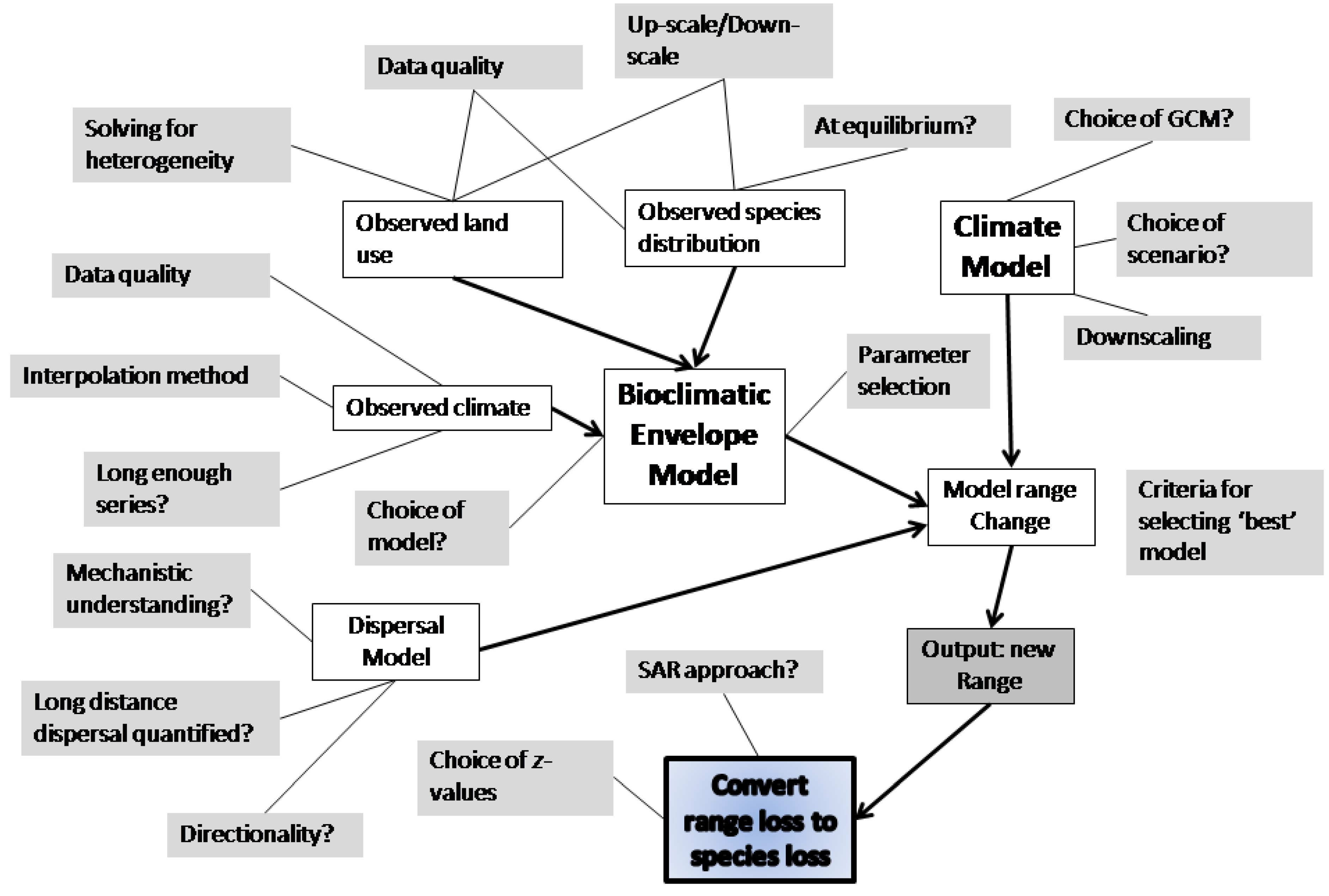
Species Distribution Models	Climate change	1. Minimal influence of evolution and phenotypic plasticity 2. Realistic spatially explicit climate scenario(s) used 3. Observed species distribution (if used) accurate and at equilibrium 4. Dispersal potential accurately captured 5. If SARs used see assumptions above
Ecosystem models	Trophic cascades	1. Trophic relationships accurately mapped 2. Causal relationships between trophic interactions well understood
Threatened species lists	Multiple interacting	1. Extinction risk criteria appropriately applied 2. Sub-criteria equally weighted 3. Subjective biases of experts understood and controlled for
Expert judgement		1. Experts biases understood and controlled 2. Interacting factors appropriately identified and weighted
Institutional capacity and ecological assessment	Biocultural	1. Key institutions/actors identified 2. Relative capacity of institutions/actors to mount conservation interventions understood and assessed 3. Ecological extinction-risk assessment accurate

In the following paragraphs I give a brief description of the main types of extinction forecasting model highlighting the key extinction drivers they seek to model and the uncertainties and assumptions that underpin them. It should be borne in mind that some of the models can be used in conjunction (e.g., species distribution models and species-area relationships) while others have a high degree of flexibility and can potentially incorporate a range of extinction drivers (e.g., multispecies metapopulation models).

I also include models where the drivers are not identified (e.g., extending trajectories of population decline) and where multiple drivers have been considered (e.g., IUCN Red list Criteria). More generally, the classification has included ‘intrinsic’ drivers where the fundamental characteristics of the population have changed (e.g., size, spatial structure) and ‘extrinsic’ drivers where some aspect of the species’ external environment has changed. Much of the uncertainty over extinction predictions in the mid-or long-term (decades to centuries) is the difficulty of accurately estimating how these intrinsic and extrinsic drivers will interact and change over time.

2.1. Simple Extrapolations

Extinction forecasting models are critically constrained by the amount and quality of information available. At one extreme are models that infer the probability of extinction from extrapolating a downward population trend or, lacking this information, from a decreasing number of confirmed sightings. Solow (2005) reviews methods based on confirmed sightings and develops a general mathematical model based on the poisson distribution for estimating the probability of extinction at time T, normally taken to be the present [9]. Roberts [6] applied Solow’s model to historical sightings of the ivory-billed woodpecker (Campephilus principalis) and concluded that at the time of its supposed rediscovery [10] the hypothesis that it was still extant should not have been rejected. The danger of using eyewitness accounts as scientific data is clearly illustrated by the many ‘sightings’ of the mythical North American Bigfoot or Sasquatch. Lozier and his colleagues recently used the numerous claims of sightings or footprints create a bioclimatic envelope model (BEM) of the present-day distribution of Bigfoot [11]. Interestingly, when they ran a model for black bear calibrated from the same region from which the Bigfoot sightings were recorded, the two models for the contemporary distribution of the two species were almost identical. These examples clearly highlight the need for regular assessments to be carried out on closed populations with a consistent survey method.

2.2. Simple Deterministic Relationships Models

For certain taxa in specific environments it is sometimes possible to identify one or more environmental variables that are strongly correlated with species numbers and which can therefore be used to make simple forecasts about future extinctions. For example, Braithewaite and Muller (1997) identified a strong historical relationship between groundwater levels and mammal numbers in northern Australia [12]. Moreover, the two periods of extremely low groundwater in this area during the 20th Century coincided with the last records of several now-extinct mammals. When combined with an analysis of traits that may make species vulnerable to the ecological consequences of low groundwater they were able to identify several species that may have a high risk of extinction.

Such correlations, if dealt with cautiously as in the above example, can undoubtedly provide useful information on species at risk but have little predictive power for at least three reasons: (1) the drivers of population decline are normally complex, multifaceted and interacting and causal relationships are often poorly understood [13]; (2) it is frequently difficult to get accurate measurements of key variables at appropriate spatial scales. If ‘refuges’ are overlooked a species may persist for many generations and ‘reappear’ when conditions are more benign. (3) Although there are often strong relationships between population decline and key environmental variables the ultimate cause of extinction is typically stochastic and a consequence of a species existing in small, isolated populations (see Section 2.3). Moreover, as Graham Caughley presciently noted, although the causes of population decline and ecological consequences of small population size are generally well known there is little evidence of these paradigms intersecting to “enlarge our idea of what is possible” in terms of a theory of extinction [14].

2.3. Population Viability Analysis

Where better data is available on the size, demographics and spatial structure of the population of a rare species, models of population viability (probability of surviving from time t1 to t2) can be constructed. Population viability analysis (PVA) has been defined by Akçakaya and Sjögren-Gulve (2000) as a “collection of methods for evaluating the threats faced by populations of species, their risks of extinction or decline, and their chances for recovery, based on species-specific data and models” [15]. PVA models generally fall into three categories: simple occupancy metapopulation models (see Section 2.4 for details of metapopulation models), structured population models and individual-based population models [15]. The latter two methods typically factor in a set of concepts revolving around the ecological consequences of small populations collectively known as the small population paradigm [14]. The basic idea is that when populations become small they are subject to a variety of stochastic processes (genetic, demographic, environmental, behavioural) that will, sooner or later, cause the extinction of the population. These processes are by no means mutually exclusive and reinforcement can occur between biotic and abiotic components leading to a so called ‘extinction vortex’ that inexorably pulls a species down into extinction [16,17]. The conceptual cohesion and the clearly interacting nature of these processes has led to the development of a range of sophisticated software packages that can model population viability.

PVA is very flexible and provides a rigorous methodology that allows conservationists to capture many uncertainties and natural variability. Moreover, its products or predictions are typically directly relevant to conservation goals. However, PVA in its more sophisticated incarnations requires a large amount of high quality data which is often not available for the very rare species that are most at risk of impending extinction. PVAs are thus most useful when they address a specific question involving a well documented species, when abundant data is available, and when they focus on relative rather than absolute results, and risks of decline rather than extinction [15].

2.4. Metapopulation Models

Of course, even rare species frequently occur in more than one population, often linked to some extent by migration. The structure and interaction between these sub-populations can also have profound influences on the probability of extinction for the metapopulation (the system of local populations) as a whole [18]. Thus, in fragmented landscapes the key conservation question shifts from minimum viable populations needed to avoid extinction to what is the minimum viable metapopulation? Recent metapopulation models of the Marsh Fritillary butterfly (Euphydryas aurinia) in the UK demonstrated that the area of land required exceeded the minimum viable metapopulation size in only 2 out of 6 extant networks of sub-populations and the remaining four networks were expected to undergo extinction within the following 15–126 years [19].

Considerable advances have also been made in modelling the metapopulation dynamics of multispecies assemblages [20] as a way of quantifying extinction debt: the deterministic extinction of species inhabiting fragments following habitat destruction [21]. Such multispecies models have given great insights into the extinction process in fragmented habitats and have propelled the concept of extinction debt into the forefront of conservation thinking [21]. However, the difficulties of parameterizing such models—especially with respect to variables such as dispersal and patch selection—to reflect real habitats means that moving beyond generalizations (e.g., poor competitors will go extinct before strong competitors) has proved challenging.

2.5. Species-Area Models

Multispecies metapopulation models (see above) rightly sit within the category of geographic models of extinction forecasting (Table 2) since they can theoretically be used to estimate extinction debt within real habitats. By far the most widely used method to calculate extinctions within habitats that have been considerably reduced in size is through the species area-relationship (SAR), one of ecology’s oldest and most general patterns [22]. This relationship can be concisely rendered using a variety of simple mathematical formulae [23], the most widely used variant being S = cA^z, where S is the number of species, A is (island) area, and z is a constant. Using the logic that a reduction in habitat area will cause an eventual and corresponding reduction in species richness (relaxation), conservationists have used the SAR in forecasting future species extinctions as a function of habitat loss due to factors such as deforestation (e.g., [24]) or future climate change (e.g., [25]). Extinction estimates are commonly generated by the simple expedient of moving down the slope of a single log SAR for a given system.

Despite the simplicity of the model and the generality of the SAR there are many potential uncertainties that make it difficult to assess the accuracy of extinction forecasts using this technique. Take, for example, the most widely known examples of predicting extinctions from studies of tropical deforestation. First, there is the problem of defining the area of a forest. This is frequently done using remote sensing algorithms that interpret the results of satellite images. Secondly, there is the problem of assessing the original species richness which, in the case of arthropods is frequently based on extrapolations from studies of host specificity and the rates of discovery of new species. Thirdly, there is the assumption that forest fragments act as virtual ‘islands’ in a ‘sea’ of uninhabitable development. This is frequently not the case and the ability of species to live and travel through the matrix of adjoining lands has a critical influence on the persistence of many species. Finally, and perhaps critically, extinction forecasts using the SAR also depends on the value chosen for the constant z, which determines the slope of the relationship. There is no strong theoretical or empirical background for the use of a single “global” slope value (although 0.25 is often chosen for such a purpose). A z-value of 0.25 is a subjective ‘middle’ value from a range of possibilities derived from analyses of true isolates and is thus unlikely to capture the slope for forest fragments and other habitat islands [26].

The species-area relationship is not the only way to model the potential impacts of area reduction on species diversity. Hubbell et al. (2008) recently used a neutral theory framework to model tree species richness and extinction risk due to habitat loss in the Brazilian Amazon [27]. Neutral theory specifies how many species are expected to be present at steady-state between speciation and extinction in the metacommunity and the expected abundances of each species. In this study the relationship between relative abundance and range size was estimated from empirical studies of nearest neighbor distances to allow estimation of the consequences of different deforestation scenarios. Extinction risk calculation was critically constrained by two major knowledge gaps. First, although tree ranges could be statistically estimated there was no way to know where these species were physically located in the Amazon. Second, as with island theory, neutral theory provides no way to estimate how different tree species would respond to different amounts of landscape transformation. Hubbell and his colleagues dealt with the first issue by randomly assigning locations to species throughout the metacommunity. The second, and more problematic, issue was dealt with by running simulations using a range of operational rules so that, under a conservative scenario, species only go extinct if their (simulated) range falls entirely within an area predicted to be heavily impacted. They study concluded that between 20% and 33% of tree species in the Brazilian Amazon would go extinct under the optimistic and nonoptimistic scenarios, respectively [27].

2.6. Species Distribution Models

Species Distribution Models relate “field observations [of presence/absence] to environmental predictor variables, based on statistically or theoretically derived response surfaces, for prediction and inference” [28]. The predictor variables are often climatic (see below) but could conceptually be any environmental variables. One of the fundamental issues in Species Distribution Models is the quality of the distributional data for the species of interest since accurate data is often missing, especially for rare and critically endangered species. Moreover, absence data is particularly problematic to obtain leading to the widespread use of pseudo-absence data (often chosen randomely from areas of presumed low suitability for the species in question [28]) for the purposes of model parameterization.

In the case of SAR-based extrapolations of extinctions using changes in climate envelopes or other types of species distribution models (SDMs) the key assumption is that area loss due to climatic/environmental unsuitability is equivalent to loss from habitat destruction [25]. While this may be true in the broadest possible sense it fails to account for the numerous uncertainties associated with both the construction of SDMs and forecasting future climate scenarios and the multiplication of uncertainties by combining these two types of models to generate extinction estimates probably renders any such forecast almost meaningless. Whittaker et al. used a schematic (Figure 1) to illustrate the large numbers of steps, assumptions and choices in such a approach to modelling extinction risk [29].

Species distribution models based on the bioclimatic envelope (also termed ‘climate space’) of the modelled species have been criticized because they fail to incorporate the many other biotic and abiotic factors that are important drivers of species distributions and the dynamics of distribution changes [29,30]. Such factors include biotic interactions, evolutionary change and dispersal ability. It is also important to note the fundamental importance of the spatial scale at which these models are applied. Pearson and Dawson argue that bioclimatic models are best applied at macro-scales, where climatic influences on species distributions dominate and where biotic interactions are much less significant [30].

Figure 1. Some of the steps, choices and assumptions involved in modelling species losses resulting from future climate change using the species distribution modelling approach. Not all studies involve all elements, e.g., land-use data, or dispersal models, but these components are important for increased realism (re-drawn from [29]).

Figure 1. Some of the steps, choices and assumptions involved in modelling species losses resulting from future climate change using the species distribution modelling approach. Not all studies involve all elements, e.g., land-use data, or dispersal models, but these components are important for increased realism (re-drawn from [29]).

2.7. Ecosystem Models

Ecosystem or trophic cascade models of extinction are defined here as any model that predicts extinction on the basis of direct or indirect impacts of removing one or more species from a food-web. The loss of one species is most likely to cause the extinction of other species that depend on it (coextinction) in the case of mutualisms and parasitism, although the effects can cascade throughout the ecosystem. Paradoxically, although this is likely to be among the most common and most predictable type of extinctions there have been very few documented examples [reviewed in 31]. Perhaps the simplest and best known example was described by Temple, who hypothesized that a coevolved obligate mutualism between the extinct dodo (Raphus cucullatus) and the very rare tambalacoque tree (Sideroxylon grandiflorum) had doomed the tree to extinction [32]. The supposed mutualism was based on the notion that seeds of the tree needed to pass through the dodo’s gut before they could germinate and supported by the fact that no seeds had germinated since the dodo’s demise more than three hundred years ago. Sadly, neither line of evidence turned out to be correct. Tambalacoque seeds germinate in low numbers without abrasion and there are several of these rare trees of less than 300 years old [33].

This type of extinction model is not restricted to simple pair-wise species interactions but also encompasses the hypothesized loss of entire functional groups. For example, da Silva and Tabarelli describe how the loss of large-gap birds and frugivorous mammals in the remaining fragments of Brazil’s Atlantic forest are predicted to cause the regional extinction of about 33.9% of trees that need these species to disperse their seeds [34]. Such simple deterministic models are arguably unable to sufficiently capture the complexities of multispecies interactions to provide precise estimates of future extinctions although they clearly have considerable heuristic value. More recently, sophisticated simulations have suggested that increased robustness and decreased levels of food web collapse are associated with higher diversity systems that have high levels of complexity, as measured by connectivity [35]. However, the development of truly predictive and robust food web models that can accurately predict the number and identity of ‘knock-on’ extinctions after the loss of one of more species remains a significant challenge.

2.8. Changes in Extinction Risk Categorization

The IUCN Red List of Threatened Species [36] is regarded as the most authoritative list of globally threatened species. At the heart of this system are a set of simple quantitative criteria based on population sizes and population decline rates, and range areas and range declines which are used to allocate species to one of several categories of extinction risk (e.g., endangered, critically endangered, extinct in the wild, etc.). It should be noted that the list employs different methods of assessing extinction risk depending on the available data and that the criteria used to assess species status are in themselves methods (e.g., PVA). In this sense it may be better to consider Red Lists as a framework for standardising and communicating extinction risk. Nevertheless, transitions between categories, on whatever basis they may have been allocated, have been used as an indicator of increasing extinction probability at a variety of spatial scales.

The key transition for extinction forecasting is between ‘endangered’ where a population has a “very high risk of extinction in the wild” to ‘critically endangered’ where the species is considered as having an “extremely high risk of extinction in the wild” [36]. The criteria for inclusion in the latter category include very small populations and geographic ranges and a strong trend of population decline. The final category (as do all categories) includes the potential for integration of results from population viability analysis: “Quantitative analysis showing the probability of extinction in the wild is at least 50% within 10 years or three generations, whichever is the longer (up to a maximum of 100 years)” [36].

Critically endangered can thus be cautiously used as a surrogate for imminent extinction. Brooke et al. tested this proposition by comparing the historical transition of bird species into the critically endangered with verified extinctions at both a global level and within Australia [37]. They concluded that species were actually going extinct at a rate 2 (Australia) to 10 (globally) times lower than predicted. The potential cause of this discrepancy was identified as the effectiveness of the global conservation community at rescuing bird species on the brink of extinction (see Section 2.9 below).

A potentially more serious issue with the IUCN Red Lists is whether the extinction risk criteria have been correctly applied. In 1997, the eminent Canadian zoologist and sea turtle expert, Nicholas Mrosovsky, accused the IUCN’s Marine Turtle Specialist Group of upgrading the listing of the Hawksbill sea turtle (Eretmochelys imbricata) without making available the scientific evidence for this change in status, and then using this to influence proposals for sustainable use of the species [38]. Thus, it is possible that unconscious or conscious biases in the information accepted and used by specialist groups might influence the categorization of species and, hence, provide an unduly pessimistic prognosis of their future survival.

Recently, the Red Lists have been used in combination with the results of bioclimatic envelope models (shifts and reductions in species’ ranges) to estimate extinction rates. A good example is the study of Bomhard et al., who computed the current and future Red List status of endemic Proteaceae in the Cape region of South Africa assuming a number of different land-use and climate change scenarios for the year 2020 [39]. The impacts of climate change were estimated using standard niche-based species distribution models (see above). They concluded that up to a third of species become more threatened (are ‘upgraded’ to a higher Red List category) under future scenarios and that under the most severe scenario the proportion of Critically Endangered taxa increases from approximately 1% to 7% and almost 2% of the 227 species will become globally Extinct. This general approach has been heavily criticised by Akçakaya et al., who argue that where such combined approaches have been adopted the Red List criteria were frequently misapplied due to arbitrary changes to spatial and temporal scales, confusion surrounding the use of spatial variables, and a widespread assumption of a linear relationship between abundance and range area [40].

2.9. Expert Judgement

Extinction predictions that incorporate multiple environmental drivers may also be derived from the reasoned judgement of experts. These sorts of forecasts have undoubtedly been the most problematic for conservation science because of a clear tendency on the part of many senior scientists to make pronouncements that appear to over-exaggerate the extinction crisis. Possibly the most famous of these pronouncements, and one that subsequently appeared in numerous intergovernmental reports, was Norman Myers ‘prediction’ in 1979 that 1 million species would be extinct by the year 2000 at a rate of 40,000 a year [1]. A year after the publication of Myers’ book Thomas Lovejoy forecast that fifteen to twenty percent of the world’s species would be extinct by the turn of the century (cited in [41]).

Such misplaced predictions of imminent demise have also been attached to a number of rare taxa. For example, Johns and Ayres proposed that an Amazonian primate, the southern bearded saki (Chiropotes satanas satanas) was already ‘beyond the brink’ in eastern Amazonia due to deforestation, hunting, its sensitivity to habitat disturbance and a dependence on many tree species valued for their timber, and would be extinct by the end of the Century [42]. Subsequent studies in the late 1990s demonstrated that the monkeys were still relatively abundant in some forest fragments where hunting was absent [43]. Of course, dire forecasts of mass extinction or of the disappearance of a specific species may influence the allocation of resources reducing the likelihood of the prediction being realized—and this is clearly often the aim.

It is this blurring between science and advocacy that makes expert predictions about extinction so difficult to assess, and possibly why so few genuine experts can be drawn into a public pronouncements. One possible solution that might reduce uncertainty and personal biases is forecasts based on the opinions of several experts filtered through a standard protocol such as the Delphi technique which uses a series of iterative questionnaires and controlled feedback from experts [44]. Such forecasts might be able to better ‘factor-in’ cultural elements such as future funding flows and the potential impacts of interventions (see 2.10 below) into the results of standard extinction models.

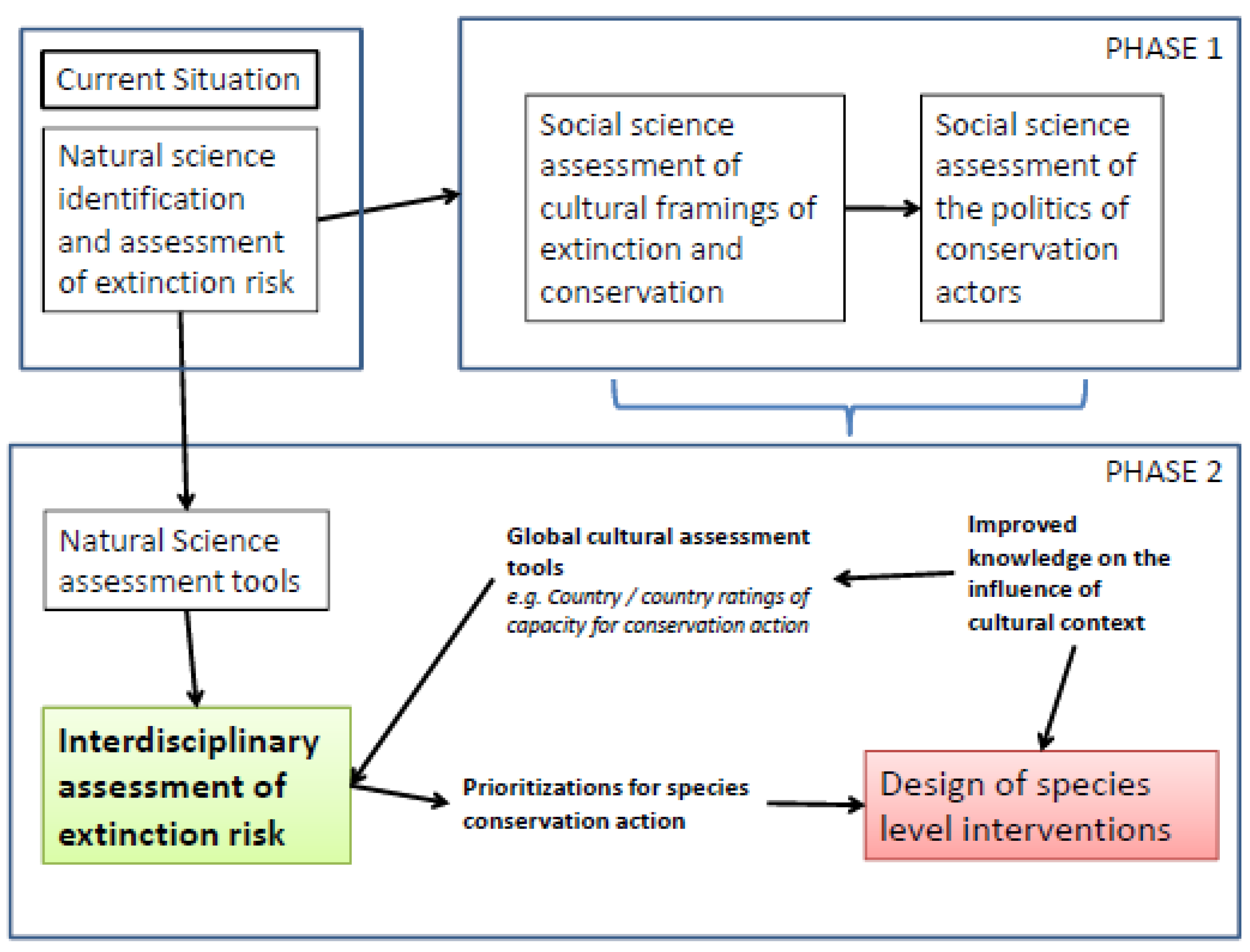
2.10. Biocultural Models

The direct role of humans in the extinction process through exploitation for food and/or trade has long been recognized as an important, if difficult to predict, component of extinction forecasting. The traditional view, derived from economic theory, was that a species would be exploited until its density fell to a level that was no longer economically viable to exploit. This view was recently challenged by Courchamp et al. who coined the term anthropogenic Allee effect to refer to the situation where the abstract value that people attach to global rarity means that the higher costs of exploiting a rare species are offset by the higher prices that ‘collectors’ or connoisseurs are willing to pay [45]. However, although there is strong evidence that the general public values rarity [46], it is equally clear that not all rare species are equally collectable. Moreover, there have been few comparative studies of the attitudes and behaviors of bird-keepers or reptile enthusiasts that drive this trade (see [47] for a rare exception]. More generally, by the same argument placing a ‘collectable’ endangered species on the IUCN Red List or on a CITES appendix could also increase the economic value of a rare species in addition to acting as a global advert alerting interested parties to this fact.

Figure 2. Schematic of proposed protocol for a phased implementation of an applied biocultural theory of avoided extinction to improve prioritization procedures (redrawn from [4]).

Figure 2. Schematic of proposed protocol for a phased implementation of an applied biocultural theory of avoided extinction to improve prioritization procedures (redrawn from [4]).

Ladle and Jepson recently took an alternative approach to assessing extinction risk by asking what factors prevent a species from becoming extinct [4]. In the modern world the safety net is provided by the global conservation movement as represented by government bodies and various international and national non-governmental conservation organizations (NGOs). However, the capacity, resources and effectiveness of organized conservation varies immensely by country and region meaning that in geographic areas where conservation capacity is low: (1) species are more likely to go extinct with appropriate interventions; (2) critically endangered species may not be effectively monitored decreasing the possibilities for emergency actions; (3) technological interventions such as captive breeding are less likely to be implemented or successful. As institutional conservation capacity is potentially measurable, Ladle and Jepson argue that a dual system of biological and institutional assessment is required to identify species with the highest risk of going extinct [4, Figure 2].

3. Conclusions

Several general conclusions can be drawn from the above brief review of contemporary extinction forecasting methods:

i. There is a great range of models available to conservationists that vary in their scope and precision. The models use different types of data, have a wide range of uncertainties and assumptions and generate predictions that can be used for different purposes. Choice of model should thus critically depend on end purpose. What will this information be used for and what level of uncertainty is acceptable? There has been a strong tendency among conservation organizations to widely disseminate extinction rate predictions made over large geographic areas based on species-area or species distribution models. Unfortunately, these models also have very high levels of uncertainty associated with their predictions leading to widespread media misrepresentation [3].

ii. There is no systematic application of different models or, more significantly, combinations of models. There is great scope for developing consensus modelling approaches which area being successfully developed in other areas of ecology [48] and may reduce some of the uncertainties. Moreover, advances are also being made in combining models. For example, Keith et al. recently successfully integrated a species distribution (habitat suitability) model with a stochastic (meta-) population model to explore the vulnerability to extinction of plants in the South African fynbos [49].

iii. The importance of the global conservation movement in avoiding extinction is acknowledged to reduce the precision of extinction forecasts [37], but there have been few attempts to incorporate this into extinction forecasting frameworks [4]. Moreover, it is clear that different types of extinction have different amounts of ‘agency’ within conservation. Thus, even though the processes leading to local extinction are identical to those that cause the global extinction of a species, the reaction of the conservation community will likely be very different. Whereas an imminent local extinction may promote some local action, an imminent global extinction may result in considerable investment of conservation resources and an emergency response from the global conservation movement. Equally, the degradation of a species rich habitat with no endemics will be far less likely to be the focus of conservation action than an equivalent area rich in endemics. Social values will thus have a significant influence of the future geography and intensity of extinction events [4].

iv. There is a strong qualitative signal from all the models—species are currently going extinct in unusual numbers [50]. Predicting their identities and focusing attention on geographic areas that are expected to suffer very high rates of extinction remains the key challenge for the global conservation movement.

v. Finally, it is important to note that although all the described methods have their limitations, they still provide important information upon which rational decisions can be made about the protection of species and environment. Indeed, while a species that is predicted to become extinct still persists (an extinction debt), there is still time for conservation to intervene and possibly reverse the situation [51]. Scientists should therefore be encouraged to continue refining and developing extinction forecasting methods [51], even with the associated risks of being overly optimistic or pessimistic.

References and Notes

1. Myers, N. The Sinking Ark; Pergamon: Oxford, UK, 2009. [Google Scholar]
2. Lomborg, B. The Skeptical Environmentalist: Measuring the State of the World; Cambridge University: Cambridge, UK, 2001; p. 252. [Google Scholar]
3. Ladle, R.J.; Jepson, P.; Araujo, M.B.; Whittaker, R.J. Dangers of crying wolf over risk of extinctions. Nature 2004, 482, 799. [Google Scholar]
4. Ladle, R.J.; Jepson, P. Towards a biocultural theory of avoided extinction. Conserv. Lett. 2008, 1, 111–118. [Google Scholar] [CrossRef]
5. Red List Categories and Criteria: Version 3.1; IUCN: Gland, Switzerland, Cambridge, UK; 2001.
6. Roberts, D.L. Extinct or possibly extinct? Science 2005, 5776, 997–998. [Google Scholar]
7. Butchart, S.H.M.; Statterfield, A.J.; Brooks, T.M. Going or gone: defining ‘Possibly Extinct’ species to give a truer picture of recent extinctions. Bull. B.O.C. 2006, 126a, 7–24. [Google Scholar]
8. Wilson, E.O. The Diversity of Life; Belknap Press: Cambridge, MA, USA, 1992. [Google Scholar]
9. Solow, A.J. Inferring extinction from a sighting record. Math. Biosci. 2005, 195, 47–55. [Google Scholar] [CrossRef]
10. Fitzpatrick, J.W.; Lammertink, M.; Luneau, M.D., Jr; Gallagher, T.W.; Harrison, B.R.; Sparling, G.M.; Rosenberg, K.V.; Rohrbaugh, R.W.; Swarthout, E.C.H.; Wrege, P.H.; Swarthout, S.B.; Dantzker, M.S.; Charif, R.A.; Barksdale, T.R.; Remsen, J.V.; Simon, S.D.; Zollner, D. Ivory-billed woodpecker (Campephilus principalis) persists in continental North America. Science 2005, 5727, 1460–1462. [Google Scholar]
11. Lozier, J.D.; Aniello, P.; Hickerson, M.J. Predicting the distribution of Sasquatch in western North America: anything goes with ecological niche modeling. J. Biogeog. 2009, 36, 1623–1627. [Google Scholar] [CrossRef]
12. Braithewaite, R.W.; Muller, W.J. Rainfall, groundwater and refuges: predicting extinctions of Australian tropical mammal species. Aust. J. Ecol. 1997, 22, 57–67. [Google Scholar] [CrossRef]
13. Norris, K. Managing threatened species: the ecological toolbox, evolutionary theory, and the declining population paradigm. J. Appl. Ecol. 2004, 41, 413–426. [Google Scholar] [CrossRef]
14. Caughley, G. Directions in conservation biology. J. Anim. Ecol. 1994, 63, 215–244. [Google Scholar] [CrossRef]
15. Akçakaya, H.R.; Sjögren-Gulve, P. Population viability analysis in conservation planning: an overview. Ecol. Bull. 2000, 48, 9–21. [Google Scholar]
16. Gilpin, M.E.; Soulé, M.E. Minimum viable populations: process of extinction. In Conservation Biology: The Science of Scarcity and Diversity; Soulé, M.E., Ed.; Sinauer Associates: Sunderland, UK, 1986; pp. 19–34. [Google Scholar]
17. Fagan, W.F.; Holmes, E.E. Quantifying the extinction vortex. Ecol. Lett. 2006, 9, 51–60. [Google Scholar]
18. Hanski, I. A practical model of metapopulation dynamics. J. Anim. Ecol. 1994, 63, 151–162. [Google Scholar] [CrossRef]
19. Bulman, C.R.; Wilson, R.J.; Holt, A.R.; Bravo, L.G.; Early, R.I.; Warren, M.S.; Thomas, C.D. Minimum viable metapopulation size, extinction debt, and the conservation of a declining species. Ecol. Appl. 2007, 17, 1460–1473. [Google Scholar] [CrossRef]
20. Tilman, D.; May, R.M.; Lehman, C.L.; Nowak, M.A. Habitat destruction and the extinction debt. Nature 1994, 371, 65–66. [Google Scholar] [CrossRef]
21. Malanson, G.P. Extinction debt: origins, developments and applications of a biogeographical trope. Prog. Phys. Geog. 2008, 32, 277–291. [Google Scholar] [CrossRef]
22. Rosenzweig, M.L. Species Diversity in Space and Time; Cambridge University: Cambridge, UK, 1995; p. 9. [Google Scholar]
23. Williams, M.R.; Lamont, B.B.; Henstridge, J.D. Species-area functions revisited. J. Biogeog. 2009, 36, 1994–2004. [Google Scholar] [CrossRef]
24. Brooks, T.M.; Mittermeier, R.A.; Mittermeier, C.G.; da Fonseca, G.A.B.; Rylands, A.B.; Konstant, W.R.; Flick, P.; Pilgrim, J.; Oldfield, S.; Magin, G.; Hilton-Taylor, C. Habitat loss and extinction in the hotspots of biodiversity. Conserv. Biol. 2002, 16, 909–923. [Google Scholar] [CrossRef]
25. Thomas, C.D.; Cameron, A.; Green, R.E.; Bakkenes, M.; Beaumont, L.J.; Collingham, Y.C.; Erasmus, B.F.N.; de Siqueira, M.F.; Grainger, A.; Hannah, L.; Hughes, L.; Huntley, B.; van Jaarsveld, A.S.; Midgley, G.F.; Miles, L.; Ortega-Huerta, M.; Peterson, A.T.; Phillips, O.L.; Williams, S.E. Extinction risk from climate change. Nature 2004, 427, 145–148. [Google Scholar] [CrossRef] [Green Version]
26. Whittaker, R.J.; Fernández-Palacios, J.M. Island Biogeography: Ecology, Evolution, and Conservation, 2nd ed.; Oxford University: Oxford, UK, 2007. [Google Scholar]
27. Hubbell, S.P.; He, F.; Condit, R.; Borda-de-Água, L.; Kellneri, J.; ter Steege, H. How many tree species are there in the Amazon and how many of them will go extinct? Proc. Natl. Acad. Sci. USA 2008, 105, 11498–11504. [Google Scholar]
28. Wisz, M.S.; Guisan, A. Do pseudo-absence selection strategies influence species distribution models and their predictions? An information-theoretic approach based on simulated data. BMC. Ecol. 2009. Available online: http://www.biomedcentral.com/1472-6785/9/8 (accessed September 30,2009).
29. Whittaker, R.J.; Araújo, M.B.; Jepson, P.; Ladle, R.J.; Watson, J.E.M.; Willis, K.J. Conservation biogeography: assessment and prospect. Divers. Distrib. 2005, 11, 3–23. [Google Scholar] [CrossRef]
30. Pearson, R.G.; Dawson, T.P. Predicting the impacts of climate change on the distribution of species: are bioclimate envelope models useful? Glob. Ecol. Biogeog. 2003, 12, 361–371. [Google Scholar] [CrossRef]
31. Dunn, R.R.; Nyeema, C.H.; Colwell, R.K.; Koh, L.P.; Sodhi, N.S. The sixth mass coextinction: are most endangered species parasites and mutualists? Proc. R. Soc. B. 2009, 276, 3037–3045. [Google Scholar] [CrossRef]
32. Temple, S.A. Plant-Animal mutualism: co-evolution with dodo leads to near extinction of plant. Science 1977, 197, 885–886. [Google Scholar]
33. Wittmer, M.C.; Cheke, A.S. The dodo and the tambalacoque tree: on obligate mutualism reconsidered. Oikos 1991, 61, 133–137. [Google Scholar] [CrossRef]
34. da Silva, J.M.C.; Tabarelli, M. Tree species impoverishment and the future flora of the Atlantic forest of northeast Brazil. Nature 2000, 404, 72–74. [Google Scholar] [CrossRef]
35. Dunne, J.A.; Williams, R.J. Cascading extinctions and community collapse in model food webs. Philos. Trans. R. Soc. B. 2009, 364, 1711–1723. [Google Scholar] [CrossRef]
36. 2001 IUCN Red List Categories and Criteria Version 3.1; The International Union for Conservation of Nature: Gland, Switzerland. Available online: www.iucnredlist.org/info/ categories criteria2001 (accessed September 30, 2009).
37. Brooke, M. de L.; Butchart, S.H.M.; Garnett, S.T.; Crowley, G.M.; Mantilla-Berniers, N.B.; Stattersfield, A.J. Rates of movement of threatened bird species between IUCN Red List categories and toward extinction. Conserv. Biol. 2008, 22, 417–427. [Google Scholar] [CrossRef]
38. Mrosovsky, N. IUCN’s credibility critically endangered. Nature 1997, 389, 436. [Google Scholar] [CrossRef]
39. Bomhard, B.; Richardson, D.M.; Donaldson, J.S. Potential impacts of future land use and climate change on the Red List status of the Proteaceae in the Cape Floristic region, South Africa. Glob. Change. Biol. 2005, 11, 1452–1468. [Google Scholar] [CrossRef]
40. Akçakaya, H.R.; Butchart, S.H.M.; Mace, G.M.; Stuart, S.N.; Hilton-Taylor, C. Use and misuse of IUCN Red List criteria in predicting climate change impacts on biodiversity. Glob. Change. Biol. 2006, 12, 2037–2043. [Google Scholar] [CrossRef]
41. Balint, P.J. How ethics shape the policy preferences of environmental scientists: what we can learn from Lomborg and his critics. Polit. Life Sci. 2003, 22, 14–23. [Google Scholar]
42. Johns, A.D.; Ayres, J.M. Southern bearded sakis—beyond the brink. Oryx 1987, 21, 164–167. [Google Scholar] [CrossRef]
43. Ferrari, S.F; Emidio-Silva, C.; Aparecida Lopes, M.; Bobadilla, U.L. Bearded sakis in south-eastern Amazonia—back from the brink? Oryx 1999, 33, 346–351. [Google Scholar]
44. Rowe, G.; Wright, G. The Delphi technique as a forecasting tool: issues and analysis. Int. J. Forecast. 1999, 15, 353–375. [Google Scholar] [CrossRef]
45. Courchamp, F.; Angulo, E.; Rivalain, P.; Hall, R.; Signoret, L.; Bull, L.; Meinard, Y. Rarity value and species extinction: the anthropogenic Allee effect. PLOS Biol. 2006, 4, e415. [Google Scholar] [CrossRef] [Green Version]
46. Angulo, E.; Deves, A.-L.; Saint Jalmes, M.; Courchamp, F. Fatal attraction: rare species in the spotlight. P. Roy. Soc. B. 2009, 276, 1331–1337. [Google Scholar] [CrossRef] [Green Version]
47. Jepson, P.; Ladle, R.J. Governing bird-keeping in Java and Bali: evidence from a household survey. Oryx 2009, 43, 364–374. [Google Scholar] [CrossRef]
48. Araújo, M.B.; Whittaker, R.J.; Ladle, R.J.; Erhard, M. Reducing uncertainty in projections of extinction-risk from climate change. Glob. Ecol. Biogeog. 2005, 14, 529–539. [Google Scholar] [CrossRef]
49. Keith, D.A.; Akçakaya, H.R.; Thuiller, W.; Midgley, G.F.; Pearson, R.G.; Phillips, S.J.; Regan, H.M.; Araújo, M.B.; Rebelo, T.G. Predicting extinction risks under climate change: coupling stochastic population models with dynamic bioclimatic habitat models. Biol. Lett. 2008, 4, 560–563. [Google Scholar] [CrossRef]
50. Pimm, S.L. The dodo went extinct (and other ecological myths). Ann. Mo. Bot. Gard. 2002, 89, 190–198. [Google Scholar] [CrossRef]
51. Kuussaari, M.; Bommarco, R.; Heikkinen, R.K.; Helm, A.; Krauss, J.; Lindborg, R.; Öckinger, E.; Pärtel, M.; Pino, J.; Rodà, F.; Stefanescu, C.; Teder, T.; Zobel, M.; Steffan-Dewenter, I. Extinction debt: a challenge for biodiversity conservation. Trends Ecol. Evol. 2009, 24, 564–571. [Google Scholar] [CrossRef]