
Fast Modeling of Binding Affinities by Means of Superposing Significant Interaction Rules (SSIR) Method


Abstract
:1. Introduction
2. Results and Discussion
2.1. Training and Cross-Validation
2.2. Inverse Structure-Activity Relationships (SAR): New Analogue Proposals
2.3. Advantages and Drawbacks of the Method
3. Material and Methods
3.1. Libraries, Sublibraries, Rules and Negation Terms
3.2. Rules Significance and Votes
3.3. Cross-Validation
4. Conclusions
Acknowledgments
Conflicts of Interest
Appendix
More Algebra among Rules
References
- Kolpak, J.; Connolly, P.J.; Lobanov, V.S.; Agrafiotis, D.K. Enhanced SAR maps: Expanding the data rendering capabilities of a popular medicinal chemistry tool. J. Chem. Inf. Model. 2009, 49, 2221–2230. [Google Scholar] [CrossRef] [PubMed]
- Wassermann, A.M.; Haebel, P.; Weskamp, N.; Bajorath, J. SAR Matrices: Automated extraction of information-rich SAR tables from large compound data sets. J. Chem. Inf. Model. 2012, 52, 1769–1776. [Google Scholar] [CrossRef] [PubMed]
- Agrafiotis, D.K.; Wiener, J.J.M.; Skalkin, A.; Kolpak, J. Single R-group polymorphisms (SRPs) and R-cliffs: An intuitive framework for analyzing and visualizing activity cliffs in a single analog series. J. Chem. Inf. Model. 2011, 51, 1122–1131. [Google Scholar] [CrossRef] [PubMed]
- Duffy, B.C.; Zhu, L.; Decornez, H.; Kitchen, D.B. Early phase drug discovery: Cheminformatics and computational techniques in identifying lead series. Bioorg. Med. Chem. 2012, 20, 5324–5342. [Google Scholar] [CrossRef] [PubMed]
- Medina-Franco, J.L.; Edwards, B.S.; Pinilla, C.; Appel, J.R.; Giulianotti, M.A.; Santos, R.G.; Yongye, A.B.; Sklar, L.A.; Houghten, R.A. Rapid scanning structure-activity relationships in combinatorial data sets: Identification of activity switches. J. Chem. Inf. Model. 2013, 53, 1475–1485. [Google Scholar] [CrossRef] [PubMed]
- Monroc, S.; Badosa, E.; Besalú, E.; Planas, M.; Bardají, E.; Montesinos, E.; Feliu, L. Improvement of cyclic decapeptides against plant pathogenic bacteria using a combinatorial chemistry approach. Peptides 2006, 27, 2575–2584. [Google Scholar] [CrossRef] [PubMed]
- Badosa, E.; Ferre, R.; Planas, M.; Feliu, L.; Besalú, E.; Cabrefiga, J.; Bardají, E.; Montesinos, E. A library of linear undecapeptides with bactericidal activity against phytopathogenic bacteria. Peptides 2007, 28, 2276–2285. [Google Scholar] [CrossRef] [PubMed]
- Feliu, L.; Oliveras, G.; Cirac, A.D.; Besalú, E.; Rosés, C.; Colomer, R.; Bardají, E.; Planas, M.; Puig, T. Antimicrobial cyclic decapeptides with anticancer activity. Peptides 2010, 31, 2017–2026. [Google Scholar] [CrossRef] [PubMed]
- Eriksson, L.; Johansson, E.; Kettaneh-Wold, N.; Wikström, C.; Wold, S. Design of Experiments. Principles and Applications; Umetrics Academy: Umea, Sweden, 2000. [Google Scholar]
- Egan, J.P. Signal Detection Theory and ROC Analysis; Academic Press: New York, NY, USA, 1975. [Google Scholar]
- Besalú, E.; De Julián Ortiz, J.V.; Pogliani, L. On Plots in QSAR/QSPR Methodologies. In Quantum Frontiers of Atoms and Molecules; Putz, M.V., Ed.; NOVA Publishing Inc.: New York, NY, USA, 2010; pp. 589–605. [Google Scholar]
- Forlay-Frick, P.; van Gyseghem, E.; Héberger, K.; Vander Heyden, Y. Selection of orthogonal chromatographic systems based on parametric and non-parametric statistical tests. Anal. Chim. Acta 2005, 539, 1–10. [Google Scholar] [CrossRef]
- Mason, S.J.; Graham, N.E. Areas beneath the relative operating characteristics (ROC) and relative operating levels (ROL) curves: Statistical significance and interpretation. Q. J. R. Meteorol. Soc. 2002, 128, 2145–2166. [Google Scholar] [CrossRef]
- Jin Cho, S.; Zheng, W.; Tropsha, A. Rational combinatorial library design. 2. Rational design of targeted combinatorial peptide libraries using chemical similarity probe and the inverse QSAR approaches. J. Chem. Inf. Comput. Sci. 1998, 38, 259–268. [Google Scholar]
- Afshar, M.; Lanoue, A.; Sallantin, J. Multiobjective/multicriteria optimization and decision support in drug discovery. Comprehens. Med. Chem. II 2007, 4, 767–774. [Google Scholar]
- King, R.D.; Muggleton, S.; Lewis, R.A.; Sternberg, M.J.E. Drug design by machine learning: The use of inductive logic programming to model the structure-activity relationships of trimethoprim analogues binding to dihydrofolate reductase. Proc. Natl. Acad. Sci. USA 1992, 89, 11322–11326. [Google Scholar] [CrossRef] [PubMed]
- Carbó, R.; Besalú, E. Nested summation symbols and perturbation theory. J. Math. Chem. 1993, 13, 331–342. [Google Scholar] [CrossRef]
- Besalú, E.; Carbó, R. Generalized Rayleigh-Schrödinger perturbation theory in Matrix form. J. Math. Chem. 1994, 15, 397–406. [Google Scholar] [CrossRef]
- Carbó, R.; Besalú, E. Definition, mathematical examples and quantum chemical applications of nested summation symbols and logical kronecker deltas. Comput. Chem. 1994, 18, 117–126. [Google Scholar] [CrossRef]
- Carbó, R.; Besalú, E. Strategies and Applications in Quantum Chemistry: From Astrophysics to Molecular Engineering Part 2; Defranceschi, M., Ellinger, Y., Eds.; Kluwer Ac. Pub.: Amsterdam, The Netherland, 1996; Volume 14, pp. 229–248. [Google Scholar]
- Besalú, E.; Ponec, R.; de Julián-Ortiz, J.V. Virtual generation of agents against mycobacterium tuberculosis: A QSAR study. Mol. Divers. 2003, 6, 107–120. [Google Scholar] [CrossRef] [PubMed]
- Barroso, J.M.; Besalú, E. Design of experiments applied to QSAR: Ranking a set of compounds and establishing a statistical significance test. Theochemistry 2005, 727, 89–96. [Google Scholar] [CrossRef]
- Yan, S.F.; Asatryan, H.; Li, J.; Zhou, Y. Novel statistical approach for primary high-throughput screening hit selection. J. Chem. Inf. Model. 2005, 45, 1784–1790. [Google Scholar] [CrossRef] [PubMed]
- Besalú, E.; Vera, l. Internal Test Sets (ITS) Method: A new cross-validation technique to assess the predictive capability of QSAR models. Application to a benchmark set of steroids. J. Chil. Chem. Soc. 2008, 53, 1576–1580. [Google Scholar] [CrossRef]
- De Julián-Ortiz, J.V.; Besalú, E.; García-Domenech, R. True prediction by consensus for small sets of cyclooxigenase-2 inhibitors. Indian J. Chem. A 2003, 42, 1392–1404. [Google Scholar]
- García-Domenech, R.; de Julián-Ortiz, J.V.; Besalú, E. True prediction of lowest observed adverse effect levels. Mol. Divers. 2006, 12, 159–168. [Google Scholar] [CrossRef] [PubMed]


| Code | R1 | R2 | R3 | R4 |
|---|---|---|---|---|
| A | R-2-naphthylmethyl | R-4-hydroxybenzyl | R-benzyl | 4-Methyl-1-cyclohexyl-methyl |
| B | S-propyl | R-2-naphthylmethyl | R-4-hydroxybenzyl | Cyclohexylpropyl |
| C | S-isopropyl | R-cyclohexyl | R-butyl | Cyclohexylmethyl |
| D | S-butyl | R-propyl | R-propyl | Cyclopentylmethyl |
| E | S-benzyl | S-hydroxymethyl | R,S-phenyl | Cycloheptylmethyl |
| F | R-butyl | S-2-butyl | Cyclobutylmethyl | |
| G | S-benzyl | S-cyclohexyl | 3-Methylpentyl | |
| H | S-isobutyl | S-benzyl | 2-Biphenyl-4-yl-ethyl | |
| I | S-propyl | 4-Tert-butyl-cyclohexylmethyl | ||
| J | 2-(3-Methoxyphenyl)-ethyl | |||
| K | 2-(4-Isobutylphenyl)-propyl | |||
| L | m-Tolylethyl | |||
| M | p-Tolylethyl | |||
| N | 2-(4-Methoxyphenyl)-ethyl | |||
| O | 2-(4-Ethoxyphenyl)-ethyl | |||
| P | Phenethyl | |||
| Q | 3-(3,4-Dimethoxyphenyl)-propyl |
| Item No. | Analogue | pKi1 a | pKi2 b |
|---|---|---|---|
| 1 | AAAA | 4.000 | 4.000 |
| 2 | AABB | 4.000 | 4.000 |
| 3 | AACA | 3.610 | 4.000 |
| 4 | ABAC | 4.000 | 4.000 |
| 5 | ABAA | 4.000 | 4.000 |
| 6 | ABBC | 4.000 | 4.000 |
| 7 | ABBB | 4.000 | 4.000 |
| 8 | ABCC | 4.000 | 4.000 |
| 9 | BBCA | 4.000 | 2.130 * |
| 10 | CBDD | 4.000 | 0.954 * |
| 11 | CBCE | 3.426 | 1.079 * |
| 12 | CBCF | 3.158 | 0.778 * |
| 13 | CCBG | 4.000 | 2.703 |
| 14 | CCBD | 4.000 | 2.262 * |
| 15 | CCBC | 4.000 | 1.839 * |
| 16 | CAAC | 2.877 | 1.000 * |
| 17 | CAAH | 2.550 * | 1.322 * |
| 18 | CABC | 3.527 | 0.778 * |
| 19 | CABH | 4.000 | 1.176 * |
| 20 | CACC | 2.978 | 0.699 * |
| 21 | CACH | 4.000 | 1.491 * |
| 22 | CDAC | 3.022 | 3.176 |
| 23 | CDAH | 2.519 * | 2.360 * |
| 24 | CDBC | 2.858 | 3.380 |
| 25 | CDBH | 1.663 * | 1.845 * |
| 26 | CDCC | 2.880 | 2.780 |
| 27 | CDCH | 2.446 * | 1.763 * |
| 28 | CBAC | 2.877 | 0.903 * |
| 29 | CBAH | 4.000 | 1.708 * |
| 30 | CBBC | 4.000 | 0.000 * |
| 31 | CBBH | 4.000 | 1.322 * |
| 32 | CBCC | 2.415 * | 0.000 * |
| 33 | CBCH | 2.822 | 1.041 * |
| 34 | BAAC | 2.585 * | 1.991 * |
| 35 | BAAH | 3.050 | 2.243 * |
| 36 | BABC | 2.639 | 2.021 * |
| 37 | BABH | 3.253 | 1.991 * |
| 38 | BACC | 3.126 | 2.212 * |
| 39 | BACH | 2.943 | 2.423 * |
| 40 | BDAC | 2.358 * | 4.000 |
| 41 | BDAH | 1.799 * | 2.772 |
| 42 | BDBC | 1.954 * | 4.000 |
| 43 | BDBH | 0.301 * | 2.210 * |
| 44 | BDCC | 2.985 | 3.778 |
| 45 | BDCH | 2.675 | 2.613 * |
| 46 | BBAC | 3.138 | 1.869 * |
| 47 | BBAH | 4.000 | 2.709 |
| 48 | BBBC | 3.366 | 1.519 * |
| 49 | BBBH | 4.000 | 2.648 |
| 50 | BBCC | 3.543 | 1.643 * |
| 51 | BBCH | 4.000 | 2.657 |
| 52 | DDBH | 0.301 * | 3.121 |
| 53 | EEEA | 3.472 | 4.000 |
| 54 | DEFA | 4.000 | 4.000 |
| 55 | DEGA | 4.000 | 4.000 |
| 56 | DDGA | 2.614 * | 3.930 |
| 57 | DEFC | 4.000 | 4.000 |
| 58 | DEFI | 3.266 | 4.000 |
| 59 | DDGF | 2.888 | 4.000 |
| 60 | DFGC | 3.368 | 4.000 |
| 61 | BEEC | 3.291 | 4.000 |
| 62 | BEEA | 3.349 | 4.000 |
| 63 | BEEH | 3.102 | 3.580 |
| 64 | DEEC | 3.740 | 4.000 |
| 65 | DEEA | 3.504 | 4.000 |
| 66 | DEEH | 3.177 | 4.000 |
| 67 | DEGH | 2.901 | 4.000 |
| 68 | BGEC | 2.941 | 4.000 |
| 69 | BGEA | 2.766 | 4.000 |
| 70 | BGEH | 2.083 * | 4.000 |
| 71 | BGGC | 2.748 | 4.000 |
| 72 | BGGA | 2.613 * | 4.000 |
| 73 | BGGH | 3.305 | 4.000 |
| 74 | BHEC | 3.788 | 3.513 |
| 75 | BHEA | 3.561 | 3.768 |
| 76 | BHEH | 2.822 | 4.000 |
| 77 | BHGC | 2.161 * | 4.000 |
| 78 | BHGA | 2.666 | 4.000 |
| 79 | BHGH | 3.054 | 4.000 |
| 80 | DGEC | 2.672 | 4.000 |
| 81 | DGEH | 1.716 * | 4.000 |
| 82 | DGGC | 2.574 * | 4.000 |
| 83 | DGGA | 2.336 * | 4.000 |
| 84 | DGGH | 2.775 | 4.000 |
| 85 | DHEC | 4.000 | 3.410 |
| 86 | DHEA | 3.226 | 4.000 |
| 87 | DHEH | 2.772 | 4.000 |
| 88 | DHGC | 2.238 * | 4.000 |
| 89 | DHGA | 2.708 | 4.000 |
| 90 | DHGH | 2.831 | 4.000 |
| 91 | EGEJ | 1.176 * | 4.000 |
| 92 | EGEK | 0.845 * | 4.000 |
| 93 | EGEH | 1.079 * | 4.000 |
| 94 | DGFJ | 1.924 * | 3.587 |
| 95 | DGEL | 1.301 * | 4.000 |
| 96 | DGEM | 1.568 * | 4.000 |
| 97 | DGEJ | 1.204 * | 4.000 |
| 98 | DGEN | 1.146 * | 4.000 |
| 99 | DGEO | 1.863 * | 4.000 |
| 100 | EGEP | 0.477 * | 4.000 |
| 101 | EGHQ | 2.691 | 4.000 |
| 102 | EGIP | 0.954 * | 4.000 |
| 103 | EGFP | 1.886 * | 4.000 |
| 104 | DDBA | 4.000 | 4.000 |
| 105 | DDBC | 1.447 * | 4.000 |
| 106 | BDBA | 4.000 | 4.000 |
| Property | Rule Order | Overall Fit | L1O | BL2O |
|---|---|---|---|---|
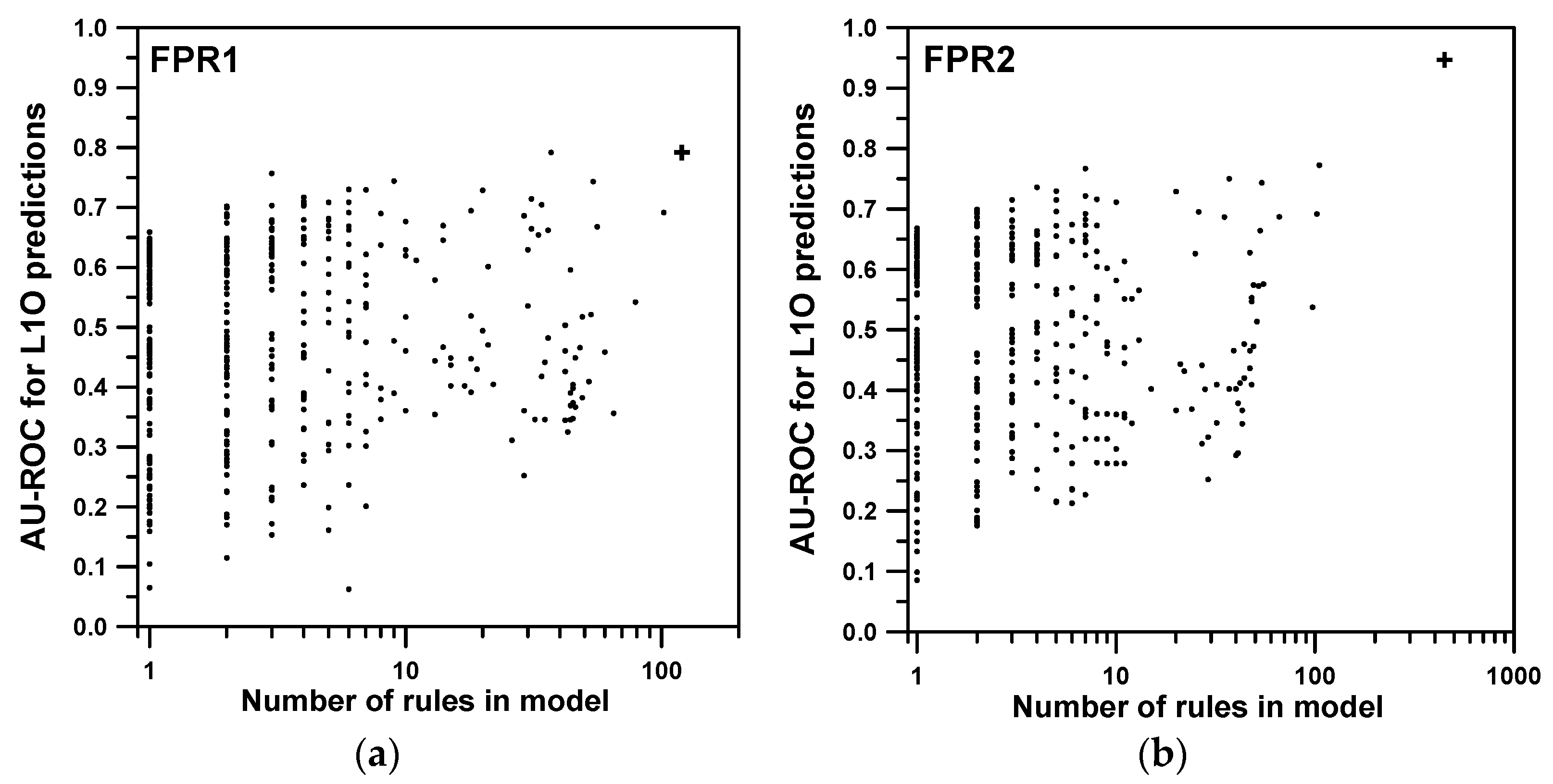
| FPR1 | 1 | 0.768 (4) | 0.761 (6) | 0.607 (6) 1408/783/177 |
| 2 | 0.894 (117) | 0.792 (171) | 0.788 (174) 1917/96/355 | |
| 3 | 0.890 (960) | 0.802 (1379) | 0.777 (1433) 1909/2/457 | |
| FPR2 | 1 | 0.934 (16) | 0.933 (18) | 0.909 (18) 2106/199/63 |
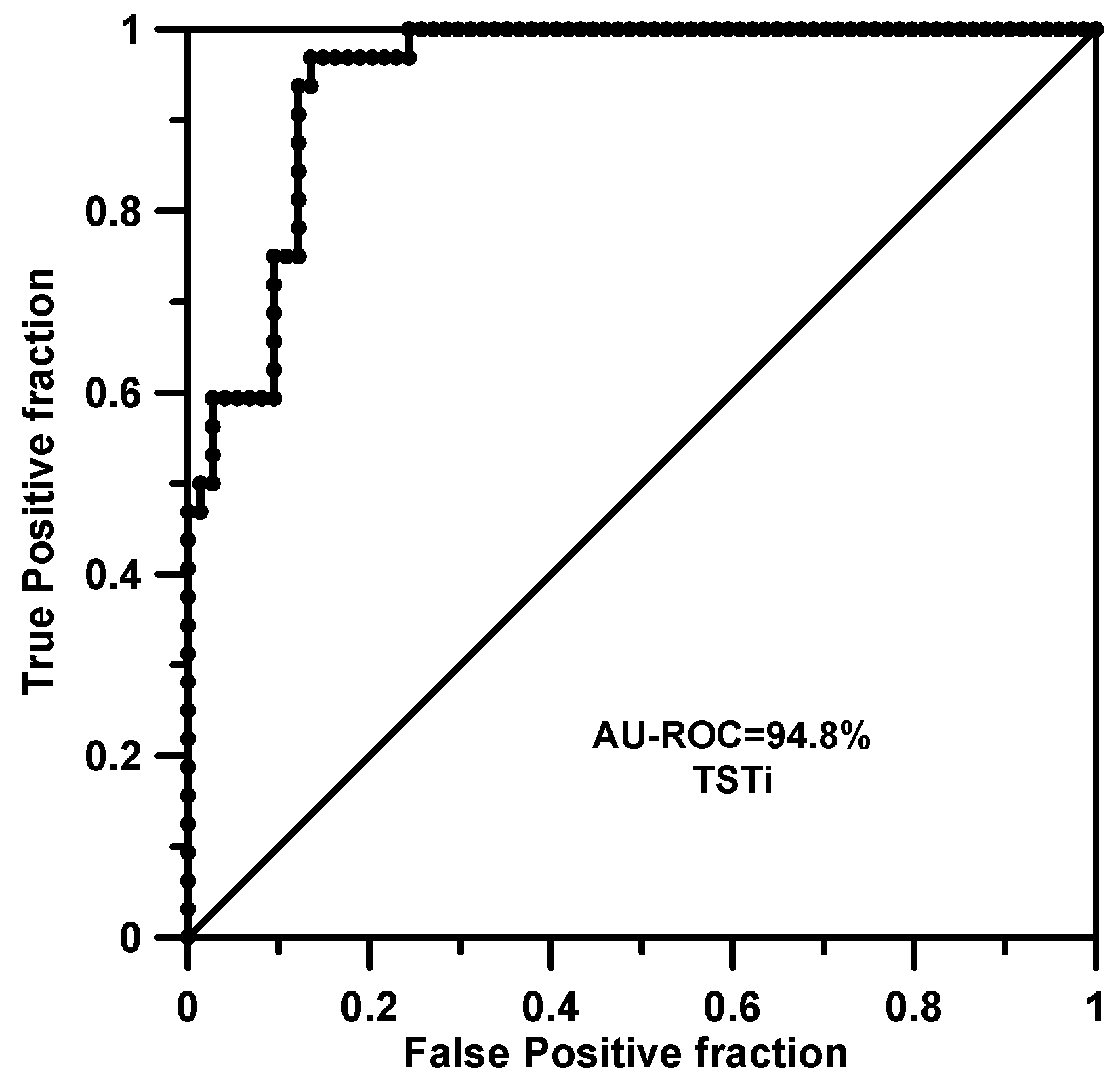
| 2 | 0.958 (447) | 0.947 (478) | 0.948 (485) 2254/2/112 | |
| 3 | 0.967 (3428) | 0.950 (3756) | 0.947 (3811) 2253/0/115 |
| Rule # | Vote | Rule | |||
|---|---|---|---|---|---|
| 1 | +1 | . | G | . | |C |
| 2 | +1 | |B | G | . | . |
| 3 | +1 | . | G | . | |Q |
| 4 | +1 | . | G | |H | . |
| 5 | −1 | . | |G | . | |K |
| 6 | +1 | . | G | . | |D |
| 7 | −1 | . | |G | |I | . |
| 8 | +1 | . | G | |C | . |
| 9 | +1 | . | G | |A | . |
| 10 | +1 | . | G | . | |F |
| 11 | +1 | . | G | . | |B |
| 12 | +1 | . | G | |D | . |
| 13 | +1 | . | G | |B | . |
| 14 | −1 | . | |G | . | |J |
| 15 | +1 | |A | G | . | . |
| 16 | −1 | . | |G | . | |P |
| 17 | +1 | |C | G | . | . |
| 18 | −1 | . | |G | . | |N |
| 19 | −1 | . | |G | . | |L |
| 20 | −1 | . | |G | . | |Q |
| 21 | +1 | . | G | . | |G |
| 22 | +1 | . | G | . | |I |
| 23 | −1 | . | |G | . | |M |
| 24 | +1 | . | G | . | |E |
| 25 | −1 | . | |G | |H | . |
| 26 | −1 | . | |G | . | |O |
| Rule # | Vote | Rule | |||
|---|---|---|---|---|---|
| 1 | −1 | |C | |A | . | . |
| 2 | −1 | |C | . | |C | . |
| 3 | +1 | C | . | . | |G |
| 4 | +1 | |D | . | |E | . |
| 5 | +1 | |D | |G | . | . |
| 6 | +1 | C | |D | . | . |
| 7 | +1 | C | . | . | |M |
| 8 | +1 | C | . | . | |N |
| 9 | +1 | C | . | . | |O |
| 10 | +1 | C | |G | . | . |
| 11 | −1 | |C | . | . | |D |
| 12 | +1 | C | . | |E | . |
| 13 | +1 | C | . | . | |P |
| 14 | +1 | C | |H | . | . |
| 15 | −1 | |C | . | . | |E |
| 16 | +1 | C | . | |G | . |
| 17 | +1 | C | . | . | |A |
| 18 | +1 | C | . | . | |Q |
| 19 | −1 | |C | . | . | |G |
| 20 | +1 | C | . | |H | . |
| 21 | +1 | C | . | |F | . |
| 22 | +1 | C | . | . | |B |
| 23 | −1 | |C | |C | . | . |
| 24 | +1 | C | . | |I | . |
| 25 | +1 | C | . | . | |J |
| 26 | +1 | C | |F | . | . |
| 27 | +1 | C | . | . | |K |
| 28 | +1 | C | . | . | |I |
| 29 | +1 | C | . | . | |L |
| 30 | +1 | C | |E | . | . |
| 31 | −1 | |C | . | |D | . |
© 2016 by the author; licensee MDPI, Basel, Switzerland. This article is an open access article distributed under the terms and conditions of the Creative Commons Attribution (CC-BY) license (http://creativecommons.org/licenses/by/4.0/).
Share and Cite
Besalú, E. Fast Modeling of Binding Affinities by Means of Superposing Significant Interaction Rules (SSIR) Method. Int. J. Mol. Sci. 2016, 17, 827. https://doi.org/10.3390/ijms17060827
Besalú E. Fast Modeling of Binding Affinities by Means of Superposing Significant Interaction Rules (SSIR) Method. International Journal of Molecular Sciences. 2016; 17(6):827. https://doi.org/10.3390/ijms17060827
Chicago/Turabian StyleBesalú, Emili. 2016. "Fast Modeling of Binding Affinities by Means of Superposing Significant Interaction Rules (SSIR) Method" International Journal of Molecular Sciences 17, no. 6: 827. https://doi.org/10.3390/ijms17060827