
Predicting Protein–Protein Interaction Sites Using Sequence Descriptors and Site Propensity of Neighboring Amino Acids

Abstract
:1. Introduction
2. Results
3. Discussion
4. Materials and Methods
4.1. Dataset
4.2. Sequence Descriptors
5. Conclusions
Acknowledgments
Author Contributions
Conflicts of Interest
Abbreviations
| PPI | Protein–Protein Interaction |
| RASA | Relative Accessible Surface Area |
| PDB | Protein Data Bank |
| SVM | Support Vector Machine |
References
- Wang, X.; Wei, X.; Thijssen, B.; Das, J.; Lipkin, S.M.; Yu, H. Three-dimensional reconstruction of protein networks provides insight into human genetic disease. Nat. Biotechnol. 2012, 30, 159–164. [Google Scholar] [CrossRef] [PubMed]
- Chagoyen, M.; Pazos, F. Characterization of clinical signs in the human interactome. Bioinformatics 2016, 32, 1761–1765. [Google Scholar] [CrossRef] [PubMed]
- Sudha, G.; Nussinov, R.; Srinivasan, N. An overview of recent advances in structural bioinformatics of Protein–Protein interactions and a guide to their principles. Progr. Biophys. Mol. Biol. 2014, 116, 141–150. [Google Scholar] [CrossRef] [PubMed]
- Mosca, R.; Pons, T.; Céol, A.; Valencia, A.; Aloy, P. Towards a detailed atlas of Protein–Protein interactions. Curr. Opin. Struct. Biol. 2013, 23, 929–940. [Google Scholar] [CrossRef] [PubMed]
- Acuner Ozbabacan, S.E.; Engin, H.B.; Gursoy, A.; Keskin, O. Transient Protein–Protein interactions. Protein Eng. Des. Sel. PEDS 2011, 24, 635–648. [Google Scholar] [CrossRef] [PubMed]
- Nooren, I.; Thornton, J.M. Structural characterisation and functional significance of transient Protein–Protein interactions. J. Mol. Biol. 2003, 325, 991–1018. [Google Scholar] [CrossRef]
- Perkins, J.R.; Diboun, I.; Dessailly, B.H.; Lees, J.G.; Orengo, C. Transient Protein–Protein interactions: Structural, functional, and network properties. Structure (Lond. Engl. 1993) 2010, 18, 1233–1243. [Google Scholar] [CrossRef] [PubMed]
- Higurashi, M.; Ishida, T.; Kinoshita, K. Identification of transient hub proteins and the possible structural basis for their multiple interactions. Protein Sci. Publ. Protein Soc. 2008, 17, 72–78. [Google Scholar] [CrossRef] [PubMed]
- Kim, P.M.; Lu, L.J.; Xia, Y.; Gerstein, M.B. Relating three-dimensional structures to protein networks provides evolutionary insights. Science 2006, 314, 1938–1941. [Google Scholar] [CrossRef] [PubMed]
- Haynes, C.; Oldfield, C.J.; Ji, F.; Klitgord, N.; Cusick, M.E.; Radivojac, P.; Uversky, V.N.; Vidal, M.; Iakoucheva, L.M. Intrinsic disorder is a common feature of hub proteins from four eukaryotic interactomes. PLoS Comput. Biol. 2006, 2, e100. [Google Scholar] [CrossRef] [PubMed]
- Singh, G.P.; Ganapathi, M.; Dash, D. Role of intrinsic disorder in transient interactions of hub proteins. Proteins 2007, 66, 761–765. [Google Scholar] [CrossRef] [PubMed]
- Esmaielbeiki, R.; Krawczyk, K.; Knapp, B.; Nebel, J.C.; Deane, C.M. Progress and challenges in predicting protein interfaces. Brief. Bioinform. 2016, 17, 117–131. [Google Scholar] [CrossRef] [PubMed]
- Chen, X.W.; Jeong, J.C. Sequence-based prediction of protein interaction sites with an integrative method. Bioinformatics 2009, 25, 585–591. [Google Scholar] [CrossRef] [PubMed]
- Wang, B.; Chen, P.; Huang, D.S.; Li, J.J.; Lok, T.M.; Lyu, M.R. Predicting protein interaction sites from residue spatial sequence profile and evolution rate. FEBS Lett. 2006, 580, 380–384. [Google Scholar] [CrossRef] [PubMed]
- Res, I.; Mihalek, I.; Lichtarge, O. An evolution based classifier for prediction of protein interfaces without using protein structures. Bioinformatics 2005, 21, 2496–2501. [Google Scholar] [CrossRef] [PubMed]
- Lovell, S.C.; Robertson, D.L. An integrated view of molecular coevolution in Protein–Protein interactions. Mol. Biol. Evol. 2010, 27, 2567–2575. [Google Scholar] [CrossRef] [PubMed]
- Pazos, F.; Helmer-Citterich, M.; Ausiello, G.; Valencia, A. Correlated mutations contain information about Protein–Protein interaction. J. Mol. Biol. 1997, 271, 511–523. [Google Scholar] [CrossRef] [PubMed]
- Ofran, Y.; Rost, B. ISIS: Interaction sites identified from sequence. Bioinformatics 2007, 23, e13–e16. [Google Scholar] [CrossRef] [PubMed]
- Murakami, Y.; Mizuguchi, K. Applying the Naïve Bayes classifier with kernel density estimation to the prediction of Protein–Protein interaction sites. Bioinformatics 2010, 26, 1841–1848. [Google Scholar] [CrossRef] [PubMed]
- Hamp, T.; Rost, B. Evolutionary profiles improve Protein–Protein interaction prediction from sequence. Bioinformatics 2015, 31, 1945–1950. [Google Scholar] [CrossRef] [PubMed]
- Park, Y.; Marcotte, E.M. Flaws in evaluation schemes for pair-input computational predictions. Nat. Methods 2012, 9, 1134–1136. [Google Scholar] [CrossRef] [PubMed]
- Hamp, T.; Rost, B. More challenges for machine-learning protein interactions. Bioinformatics 2015, 31, 1521–1525. [Google Scholar] [CrossRef] [PubMed]
- Kawashima, S.; Kanehisa, M. AAindex: Amino Acid index database. Nucleic Acids Res. 2000, 28, 374. [Google Scholar] [CrossRef] [PubMed]
- Kawashima, S.; Pokarowski, P.; Pokarowska, M.; Kolinski, A.; Katayama, T.; Kanehisa, M. AAindex: Amino acid index database, progress report 2008. Nucleic Acids Res. 2008, 36, 202–205. [Google Scholar] [CrossRef] [PubMed]
- Nakai, K.; Kidera, A.; Kanehisa, M. Cluster analysis of amino acid indices for prediction of protein structure and function. Protein Eng. 1988, 2, 93–100. [Google Scholar] [CrossRef] [PubMed]
- Tomii, K.; Kanehisa, M. Analysis of amino acid indices and mutation matrices for sequence comparison and structure prediction of proteins. Protein Eng. 1996, 9, 27–36. [Google Scholar] [CrossRef] [PubMed]
- Gallet, X.; Charloteaux, B.; Thomas, A.; Brasseur, R. A fast method to predict protein interaction sites from sequences1. J. Mol. Biol. 2000, 302, 917–926. [Google Scholar] [CrossRef] [PubMed]
- Chou, K.C. Prediction of protein cellular attributes using pseudo-amino acid composition. Proteins 2001, 43, 246–255. [Google Scholar] [CrossRef] [PubMed]
- Chou, K.C.; Cai, Y.D. Predicting protein quaternary structure by pseudo amino acid composition. Proteins 2003, 53, 282–289. [Google Scholar] [CrossRef] [PubMed]
- Zhang, S.W.; Pan, Q.; Zhang, H.C.; Shao, Z.C.; Shi, J.Y. Prediction of protein homo-oligomer types by pseudo amino acid composition: Approached with an improved feature extraction and Naive Bayes Feature Fusion. Amino Acids 2006, 30, 461–468. [Google Scholar] [CrossRef] [PubMed]
- Jia, J.; Liu, Z.; Xiao, X.; Liu, B.; Chou, K.C. iPPBS-Opt: A sequence-based ensemble classifier for identifying Protein–Protein binding sites by optimizing imbalanced training datasets. Mol. (Basel, Switz.) 2016, 21, 95. [Google Scholar] [CrossRef] [PubMed]
- Jia, J.; Liu, Z.; Xiao, X.; Liu, B.; Chou, K.C. iPPI-Esml: An ensemble classifier for identifying the interactions of proteins by incorporating their physicochemical properties and wavelet transforms into PseAAC. J. Theor. Biol. 2015, 377, 47–56. [Google Scholar] [CrossRef] [PubMed]
- Jia, J.; Liu, Z.; Xiao, X.; Liu, B.; Chou, K.C. Identification of Protein–Protein binding sites by incorporating the physicochemical properties and stationary wavelet transforms into pseudo amino acid composition. J. Biomol. Struct. Dyn. 2016, 34, 1946–1961. [Google Scholar] [CrossRef] [PubMed]
- Ashkenazy, H.; Erez, E.; Martz, E.; Pupko, T.; Ben-Tal, N. ConSurf 2010: Calculating evolutionary conservation in sequence and structure of proteins and nucleic acids. Nucleic Acids Res. 2010, 38, W529–W533. [Google Scholar] [CrossRef] [PubMed]
- Celniker, G.; Nimrod, G.; Ashkenazy, H.; Glaser, F.; Martz, E.; Mayrose, I. Consurf: Using evolutionary data to raise testable hypotheses about protein function. Israel J. Chem. 2013, 53, 199–206. [Google Scholar] [CrossRef]
- Pupko, T.; Bell, R.E.; Mayrose, I.; Glaser, F.; Ben-Tal, N. Rate4Site: An algorithmic tool for the identification of functional regions in proteins by surface mapping of evolutionary determinants within their homologues. Bioinformatics 2002, 18, S71–S77. [Google Scholar] [CrossRef] [PubMed]
- Zhou, H.X.; Qin, S. Interaction-site prediction for protein complexes: A critical assessment. Bioinformatics 2007, 23, 2203–2209. [Google Scholar] [CrossRef] [PubMed]
- Chou, K.C. Some remarks on protein attribute prediction and pseudo amino acid composition. J. Theor. Biol. 2011, 273, 236–247. [Google Scholar] [CrossRef] [PubMed]
- Chen, W.; Ding, H.; Feng, P.; Lin, H.; Chou, K.C. iACP: A sequence-based tool for identifying anticancer peptides. Oncotarget 2016, 7, 16895–16909. [Google Scholar] [CrossRef] [PubMed]
- Chen, W.; Feng, P.; Ding, H.; Lin, H.; Chou, K.C. Using deformation energy to analyze nucleosome positioning in genomes. Genomics 2016, 107, 69–75. [Google Scholar] [CrossRef] [PubMed]
- Jia, J.; Liu, Z.; Xiao, X.; Liu, B.; Chou, K.C. iSuc-PseOpt: Identifying lysine succinylation sites in proteins by incorporating sequence-coupling effects into pseudo components and optimizing imbalanced training dataset. Anal. Biochem. 2016, 497, 48–56. [Google Scholar] [CrossRef] [PubMed]
- Jia, J.; Liu, Z.; Xiao, X.; Liu, B.; Chou, K.C. pSuc-Lys: Predict lysine succinylation sites in proteins with PseAAC and ensemble random forest approach. J. Theor. Biol. 2016, 394, 223–230. [Google Scholar] [CrossRef] [PubMed]
- Jia, J.; Liu, Z.; Xiao, X.; Liu, B.; Chou, K.C. iCar-PseCp: Identify carbonylation sites in proteins by Monte Carlo sampling and incorporating sequence coupled effects into general PseAAC. Oncotarget 2016, 7, 34558–34570. [Google Scholar] [CrossRef] [PubMed]
- Liu, B.; Fang, L.; Liu, F.; Wang, X.; Chou, K.C. iMiRNA-PseDPC: MicroRNA precursor identification with a pseudo distance-pair composition approach. J. Biomol. Struct. Dyn. 2016, 34, 223–235. [Google Scholar] [CrossRef] [PubMed]
- Liu, B.; Fang, L.; Long, R.; Lan, X.; Chou, K.C. iEnhancer-2L: A two-layer predictor for identifying enhancers and their strength by pseudo κ-tuple nucleotide composition. Bioinformatics 2016, 32, 362–369. [Google Scholar] [CrossRef] [PubMed]
- Liu, B.; Long, R.; Chou, K.C. iDHS-EL: Identifying DNase I hypersensitive sites by fusing three different modes of pseudo nucleotide composition into an ensemble learning framework. Bioinformatics 2016, 32, 2411–2418. [Google Scholar] [CrossRef] [PubMed]
- Liu, Z.; Xiao, X.; Yu, D.J.; Jia, J.; Qiu, W.R.; Chou, K.C. pRNAm-PC: Predicting N6-methyladenosine sites in RNA sequences via physical-chemical properties. Anal. Biochem. 2016, 497, 60–67. [Google Scholar] [CrossRef] [PubMed]
- Qiu, W.R.; Xiao, X.; Xu, Z.C.; Chou, K.C. iPhos-PseEn: Identifying phosphorylation sites in proteins by fusing different pseudo components into an ensemble classifier. Oncotarget 2016, 7, 51270–51283. [Google Scholar] [CrossRef] [PubMed]
- Xiao, X.; Ye, H.X.; Liu, Z.; Jia, J.H.; Chou, K.C. iROS-gPseKNC: Predicting replication origin sites in DNA by incorporating dinucleotide position-specific propensity into general pseudo nucleotide composition. Oncotarget 2016, 7, 34180–34189. [Google Scholar] [CrossRef] [PubMed]
- Ganganwar, V. An overview of classification algorithms for imbalanced data sets. Int. J. Emerg. Technol. Adv. Eng. 2012, 2, 42–47. [Google Scholar]
- Gribskov, M.; Robinson, N.L. Use of receiver operating characteristic (ROC) analysis to evaluate sequence matching. Comput. Chem. 1996, 20, 25–33. [Google Scholar] [CrossRef]
- Liu, R.; Jiang, W.; Zhou, Y. Identifying Protein–Protein interaction sites in transient complexes with temperature factor, sequence profile and accessible surface area. Amino Acids 2010, 38, 263–270. [Google Scholar] [CrossRef] [PubMed]
- Dhole, K.; Singh, G.; Pai, P.P.; Mondal, S. Sequence-based prediction of Protein–Protein interaction sites with L1-logreg classifier. J. Theor. Biol. 2014, 348, 47–54. [Google Scholar] [CrossRef] [PubMed]
- Chou, K.C.; Shen, H.B. Recent advances in developing web-servers for predicting protein attributes. Nat. Sci. 2009, 1, 63–92. [Google Scholar] [CrossRef]
- Chou, K.C. Impacts of bioinformatics to medicinal chemistry. Med. Chem. 2015, 11, 218–234. [Google Scholar] [CrossRef] [PubMed]
- Chen, W.; Lin, H.; Chou, K.C. Pseudo nucleotide composition or PseKNC: An effective formulation for analyzing genomic sequences. Mol. BioSyst. 2015, 11, 2620–2634. [Google Scholar] [CrossRef] [PubMed]
- Qiu, W.R.; Sun, B.Q.; Xiao, X.; Xu, Z.C.; Chou, K.C. iHyd-PseCp: Identify hydroxyproline and hydroxylysine in proteins by incorporating sequence-coupled effects into general PseAAC. Oncotarget 2016, 7, 44310–44321. [Google Scholar] [CrossRef] [PubMed]
- Zhang, C.J.; Tang, H.; Li, W.C.; Lin, H.; Chen, W.; Chou, K.C. iOri-Human: Identify human origin of replication by incorporating dinucleotide physicochemical properties into pseudo nucleotide composition. Oncotarget 2016, 5. [Google Scholar] [CrossRef] [PubMed]
- Chen, Y.K.; Li, K.B. Predicting membrane protein types by incorporating protein topology, domains, signal peptides, and physicochemical properties into the general form of Chou’s pseudo amino acid composition. J. Theor. Biol. 2013, 318, 1–12. [Google Scholar] [CrossRef] [PubMed]
- Zhang, J.; Zhao, X.; Sun, P.; Ma, Z. PSNO: Predicting cysteine S-nitrosylation sites by incorporating various sequence-derived features into the general form of Chou’s PseAAC. Int. J. Mol. Sci. 2014, 15, 11204–11219. [Google Scholar] [CrossRef] [PubMed]
- Berman, H.M.; Westbrook, J.; Feng, Z.; Gilliland, G.; Bhat, T.N.; Weissig, H.; Shindyalov, I.N.; Bourne, P.E. The protein data bank. Nucleic Acids Res. 2000, 28, 235–242. [Google Scholar] [CrossRef] [PubMed]
- Chung, J.L.; Wang, W.; Bourne, P.E. Exploiting sequence and structure homologs to identify Protein–Protein binding sites. Proteins 2006, 62, 630–640. [Google Scholar] [CrossRef] [PubMed]
- Yan, C.; Dobbs, D.; Honavar, V. A two-stage classifier for identification of Protein–Protein interface residues. Bioinformatics 2004, 20, 371–378. [Google Scholar] [CrossRef] [PubMed]
- del Sol Mesa, A.; Pazos, F.; Valencia, A. Automatic methods for predicting functionally important residues. J. Mol. Biol. 2003, 326, 1289–1302. [Google Scholar] [CrossRef]
- Ezkurdia, I.; Bartoli, L.; Fariselli, P.; Casadio, R.; Valencia, A.; Tress, M.L. Progress and challenges in predicting Protein–Protein interaction sites. Brief. Bioinform. 2009, 10, 233–246. [Google Scholar] [CrossRef] [PubMed]
- Altschul, S.F.; Madden, T.L.; Schaffer, A.A.; Zhang, J.; Zhang, Z.; Miller, W. Gapped blast and PSI-BLAST: A new generation of protein database search programs. Nucleic Acids Res. 1997, 25, 3389–3402. [Google Scholar] [CrossRef] [PubMed]
- Dosztányi, Z.; Mészáros, B.; Simon, I. ANCHOR: Web server for predicting protein binding regions in disordered proteins. Bioinformatics 2009, 25, 2745–2746. [Google Scholar] [CrossRef] [PubMed]
- Ansari, S.; Helms, V. Statistical analysis of predominantly transient Protein–Protein interfaces. Proteins 2005, 61, 344–355. [Google Scholar] [CrossRef] [PubMed]
- Potenza, E.; Di Domenico, T.; Walsh, I.; Tosatto, S.C.E. MobiDB 2.0: An improved database of intrinsically disordered and mobile proteins. Nucleic Acids Res. 2015, 43, D315–D320. [Google Scholar] [CrossRef] [PubMed]
- Schäffer, A.A.; Aravind, L.; Madden, T.L.; Shavirin, S.; Spouge, J.L.; Wolf, Y.I.; Koonin, E.V.; Altschul, S.F. Improving the accuracy of PSI-BLAST protein database searches with composition-based statistics and other refinements. Nucleic Acids Res. 2001, 29, 2994–3005. [Google Scholar] [CrossRef] [PubMed]
- Rao, V.S.; Srinivas, K.; Sujini, G.N.; Kumar, G.N.S. Protein–Protein interaction detection: Methods and analysis. Int. J. Proteom. 2014, 2014, 1–12. [Google Scholar] [CrossRef] [PubMed]
- Mika, S.; Rost, B. Protein–Protein interactions more conserved within species than across species. PLoS Comput. Biol. 2006, 2, e79. [Google Scholar] [CrossRef] [PubMed]
- Bitbol, A.F.; Dwyer, R.S.; Colwell, L.J.; Wingreen, N.S. Inferring interaction partners from protein sequences. Proc. Natl. Acad. Sci. USA 2016. [Google Scholar] [CrossRef] [PubMed]
- Li, W.; Godzik, A. Cd-hit: A fast program for clustering and comparing large sets of protein or nucleotide sequences. Bioinformatics 2006, 22, 1658–1659. [Google Scholar] [CrossRef] [PubMed]
- Larkin, M.A.; Blackshields, G.; Brown, N.P.; Chenna, R.; McGettigan, P.A.; McWilliam, H.; Valentin, F.; Wallace, I.M.; Wilm, A.; Lopez, R.; et al. Clustal W and Clustal X version 2.0. Bioinformatics 2007, 23, 2947–2948. [Google Scholar] [CrossRef] [PubMed]
- Felsenstein, J. PHYLIP (Phylogeny Inference Package) Version 3.6; Distributed by the Author; Department of Genome Sciences, University of Washington: Seattle, WA, USA, 2005. [Google Scholar]
- Janin, J.; Wodak, S. The third CAPRI assessment meeting Toronto, Canada, April 20–21, 2007. Structure 2007, 15, 755–759. [Google Scholar] [CrossRef] [PubMed]
- Koike, A.; Takagi, T. Prediction of protein–protein interaction sites using support vector machines. Protein Eng. Des. Sel. 2004, 17, 165–173. [Google Scholar] [CrossRef] [PubMed]
- del Sol Mesa, A.; Pazos, F.; Valencia, A. PhosphoSVM: Prediction of phosphorylation sites by integrating various protein sequence attributes with a support vector machine. J. Mol. Biol. 2003, 326, 1289–1302. [Google Scholar] [CrossRef]
- Johansson, F.; Toh, H. A comparative study of conservation and variation scores. BMC Bioinform. 2010, 11, 388. [Google Scholar] [CrossRef] [PubMed]
- Karlin, S.; Brocchieri, L. Evolutionary conservation of RecA genes in relation to protein structure and function. J. Bacteriol. 1996, 178, 1881–1894. [Google Scholar] [PubMed]
- Capra, J.A.; Singh, M. Predicting functionally important residues from sequence conservation. Bioinformatics 2007, 23, 1875–1882. [Google Scholar] [CrossRef] [PubMed]
- Sander, C.; Schneider, R. Database of homology-derived protein structures and the structural meaning of sequence alignment. Proteins 1991, 9, 56–68. [Google Scholar] [CrossRef] [PubMed]
- Kim, H.; Park, H. Protein secondary structure prediction based on an improved support vector machines approach. Protein Eng. 2003, 16, 553–560. [Google Scholar] [CrossRef] [PubMed]
- Wang, Z.; Zhao, F.; Peng, J.; Xu, J. Protein 8-class secondary structure prediction using conditional neural fields. Proteomics 2011, 11, 3786–3792. [Google Scholar] [CrossRef] [PubMed]
- Petersen, B.; Petersen, T.N.; Andersen, P.; Nielsen, M.; Lundegaard, C. A generic method for assignment of reliability scores applied to solvent accessibility predictions. BMC Struct. Biol. 2009, 9, 51. [Google Scholar] [CrossRef] [PubMed]
- Atchley, W.R.; Zhao, J.; Fernandes, A.D.; Drüke, T. Solving the protein sequence metric problem. Proc. Natl. Acad. Sci. USA 2005, 102, 6395–6400. [Google Scholar] [CrossRef] [PubMed]
- Hansen, J.C.; Lu, X.; Ross, E.D.; Woody, R.W. Intrinsic protein disorder, amino acid composition, and histone terminal domains. J. Biol. Chem. 2006, 281, 1853–1856. [Google Scholar] [CrossRef] [PubMed]
- Forman-Kay, J.D.; Mittag, T. From sequence and forces to structure, function, and evolution of intrinsically disordered proteins. Struct. (Lond. Engl. 1993) 2013, 21, 1492–1499. [Google Scholar] [CrossRef] [PubMed]
- Momen-Roknabadi, A.; Sadeghi, M.; Pezeshk, H.; Marashi, S.A. Impact of residue accessible surface area on the prediction of protein secondary structures. BMC Bioinform. 2008, 9. [Google Scholar] [CrossRef] [PubMed]
- Bordner, A.J.; Abagyan, R. Statistical analysis and prediction of Protein–Protein interfaces. Proteins 2005, 60, 353–366. [Google Scholar] [CrossRef] [PubMed]
- Sikić, M.; Tomić, S.; Vlahovicek, K. Prediction of Protein–Protein interaction sites in sequences and 3D structures by random forests. PLoS Comput. Biol. 2009, 5, e1000278. [Google Scholar] [CrossRef] [PubMed]
- Vapnik, V.N. The Nature of Statistical Learning Theory; Springer: New York, NY, USA, 1995. [Google Scholar]
- You, Z.H.; Lei, Y.K.; Zhu, L.; Xia, J.; Wang, B. Prediction of Protein–Protein interactions from amino acid sequences with ensemble extreme learning machines and principal component analysis. BMC Bioinform. 2013, 14, S10. [Google Scholar] [CrossRef] [PubMed]
- Das, R.; Dimitrova, N.; Xuan, Z.; Rollins, R.A.; Haghighi, F.; Edwards, J.R.; Ju, J.; Bestor, T.H.; Zhang, M.Q. Computational prediction of methylation status in human genomic sequences. Proc. Natl. Acad. Sci. USA 2006, 103, 10713–10716. [Google Scholar] [CrossRef] [PubMed]
- Cai, Y.D.; Liu, X.J.; Xu, X.B.; Chou, K.C. Support vector machines for prediction of protein subcellular location by incorporating quasi-sequence-order effect. J. Cell. Biochem. 2002, 84, 343–348. [Google Scholar] [CrossRef] [PubMed]
- Chang, C.C.; Lin, C.J. LIBSVM: A library for support vector machines. ACM Trans. Intell. Syst. Technol. 2011, 2, 1–27. [Google Scholar] [CrossRef]


| Secondary Structure | Interaction Sites | Non-interaction Sites | Total |
|---|---|---|---|
| helix | 875 (728) | 5717 (2973) | 6592 (3701) |
| sheet | 803 (630) | 3845 (1619) | 4648 (2249) |
| other | 2751 (2428) | 10,933 (7315) | 13,684 (9743) |
| total | 4429 (3786) | 20,495 (11,907) | 24,924 (15,693) |
| Prediction Methods | Recall | Precision | Accuracy | Description |
|---|---|---|---|---|
| Liu et al. 2010 [52] | 0.597 | 0.407 | 0.630 | B-factors were used as the feature for prediction |
| this study | 0.597 | 0.311 | 0.583 | only sequence-derived features were used |
| PDB IDs and the Percentage of Amino Acid Residues in Disorder Regions | ||||
|---|---|---|---|---|
| 1A4Y_A (6.1) | 1ABR_A (3.2) | 1ABR_B (3.2) | 1ACB_I (n.a.) | 1AHW_B (21.9) |
| 1AHW_C (44.3) | 1AK4_A (8.6) | 1AK4_D (4.2) | 1ATN_D (7.7) | 1AVG_H (11.2) |
| 1AVG_I (10.0) | 1AVW_B (3.0) | 1AVZ_B (25.2) | 1AVZ_C (10.8) | 1AY7_A (7.3) |
| 1AY7_B (n.a.) | 1AZS_B (18.5) | 1AZS_C (6.4) | 1AZZ_C (3.5) | 1B6C_A (4.7) |
| 1B6C_B (n.a.) | 1B7Y_A (1.1) | 1B7Y_B (6.6) | 1BDJ_A (3.7) | 1BDJ_B (n.a) |
| 1BGX_T (5.7) | 1BI7_A (23.1) | 1BI7_B (n.a) | 1BI8_B (17.5) | 1BMQ_A (9.4) |
| 1BMQ_B (n.a.) | 1BP3_A (30.4) | 1BP3_B (n.a.) | 1BRB_I (n.a.) | 1BRS_A (11.5) |
| 1BVK_A (n.a.) | 1BVK_C (n.a.) | 1BVN_P (8.6) | 1BVN_T (n.a.) | 1CA0_B (30.0) |
| 1CGI_I (11.4) | 1CXZ_B (18.6) | 1D4V_A (41.4) | 1D4V_B (24.5) | 1DAN_L (6.4) |
| 1DAN_T (15.3) | 1DAN_U (n.a.) | 1DFJ_E (2.1) | 1DHK_B (4.9) | 1E96_A (3.13) |
| 1E96_B (25.5) | 1E9H_B (n.a.) | 1EAY_C (10.0) | 1EFU_A (2.8) | 1EFU_B (4.3) |
| 1ETH_A (3.1) | 1ETH_B (5.3) | 1FAP_B (8.0) | 1FLE_I (31.6) | 1FLT_V (18.1) |
| 1FLT_Y (6.4) | 1FQ1_A (17.0) | 1FSS_B (3.6) | 1GFW_A (18.0) | 1GFW_B (n.a.) |
| 1GLA_F (3.2) | 1GLA_G (5.3) | 1GOT_B (9.7) | 1GOT_G (2.9) | 1GPQ_A (9.5) |
| 1GUA_B (26.5) | 1HE8_A (8.4) | 1HJA_C (3.2) | 1HLU_A (6.4) | 1HLU_P (7.2) |
| 1HWH_B (26.3) | 1IRA_X (n.a.) | 1IRA_Y (3.4) | 1ITB_A (2.6) | 1JSU_C (31.0) |
| 1KIG_I (16.9) | 1KKL_A (2.5) | 1KKL_H (6.9) | 1KXV_C (0.6) | 1L0Y_A (13.9) |
| 1L0Y_B (2.4) | 1MAH_A (21.3) | 1NOC_A (7.9) | 1NOC_B (4.6) | 1PDK_A (5.4) |
| 1PDK_B (12.4) | 1PYT_A (2.9) | 1PYT_B (6.3) | 1QBK_B (9.3) | 1QBK_C (6.3) |
| 1SGP_E (n.a.) | 1SMP_A (6.7) | 1SMP_I (3.4) | 1SPB_P (n.a.) | 1STF_E (3.2) |
| 1STF_I (40.8) | 1TAB_I (1.2) | 1TCO_A (19.4) | 1TMQ_B (6.5) | 1UDI_E (14.3) |
| 1UDI_I (n.a.) | 1UEA_A (n.a.) | 1UEA_B (n.a.) | 1UGH_E (n.a.) | 1UUZ_A (19.0) |
| 1VAD_A (5.9) | 1VAD_B (14.9) | 1WQ1_G (9.5) | 1XDT_R (9.3) | 1XDT_T (33.1) |
| 1ZBD_A (44.3) | 1ZBD_B (20.9) | 2KAI_B (4.1) | 2PCC_A (18.4) | 2PCC_B (13.3) |
| 2SIC_I (15.4) | 2SNI_I (34.5) | 2TEC_E (8.6) | 3SGB_I (10.0) | 3TGI_I (13.0) |
| 4SGB_I (8.5) | 7CEI_A (28.7) | 7CEI_B(54.0) | ||
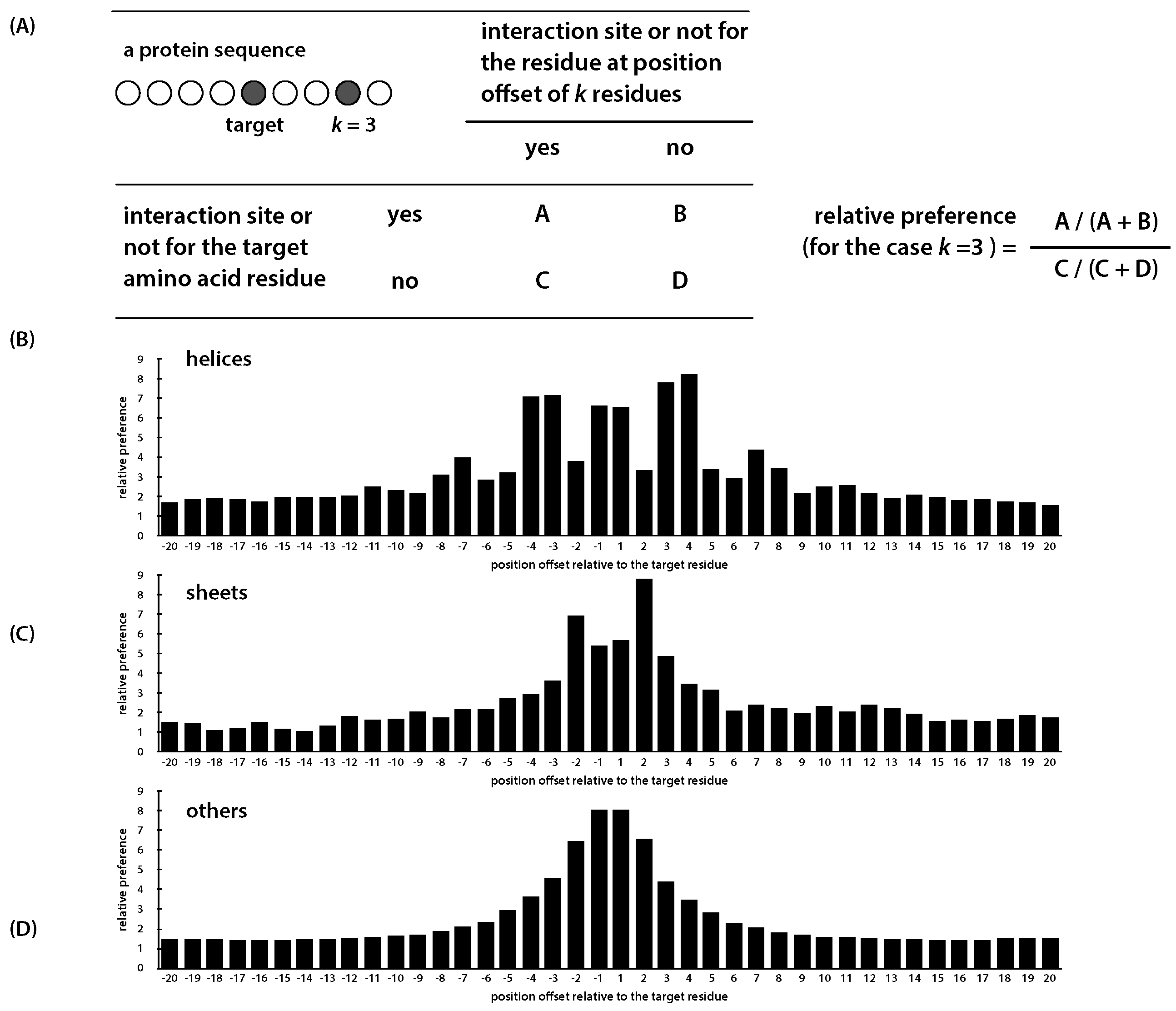
| Secondary Structure | +1 | +2 | +3 | +4 | ||||
|---|---|---|---|---|---|---|---|---|
| helix | 7.081 | 7.172 | 3.817 | 6.642 | 6.575 | 3.359 | 7.823 | 8.241 |
| sheet | 2.924 | 3.621 | 6.902 | 5.391 | 5.673 | 8.793 | 4.859 | 3.463 |
| other | 3.620 | 4.576 | 6.491 | 8.035 | 8.071 | 6.602 | 4.428 | 3.478 |
© 2016 by the authors; licensee MDPI, Basel, Switzerland. This article is an open access article distributed under the terms and conditions of the Creative Commons Attribution (CC-BY) license (http://creativecommons.org/licenses/by/4.0/).
Share and Cite
Kuo, T.-H.; Li, K.-B. Predicting Protein–Protein Interaction Sites Using Sequence Descriptors and Site Propensity of Neighboring Amino Acids. Int. J. Mol. Sci. 2016, 17, 1788. https://doi.org/10.3390/ijms17111788
Kuo T-H, Li K-B. Predicting Protein–Protein Interaction Sites Using Sequence Descriptors and Site Propensity of Neighboring Amino Acids. International Journal of Molecular Sciences. 2016; 17(11):1788. https://doi.org/10.3390/ijms17111788
Chicago/Turabian StyleKuo, Tzu-Hao, and Kuo-Bin Li. 2016. "Predicting Protein–Protein Interaction Sites Using Sequence Descriptors and Site Propensity of Neighboring Amino Acids" International Journal of Molecular Sciences 17, no. 11: 1788. https://doi.org/10.3390/ijms17111788
APA StyleKuo, T.-H., & Li, K.-B. (2016). Predicting Protein–Protein Interaction Sites Using Sequence Descriptors and Site Propensity of Neighboring Amino Acids. International Journal of Molecular Sciences, 17(11), 1788. https://doi.org/10.3390/ijms17111788