Probing the Nanosecond Dynamics of a Designed Three-Stranded Beta-Sheet with a Massively Parallel Molecular Dynamics Simulation

Abstract
:
1. Introduction
2. Results and Discussion
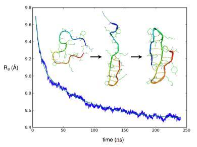
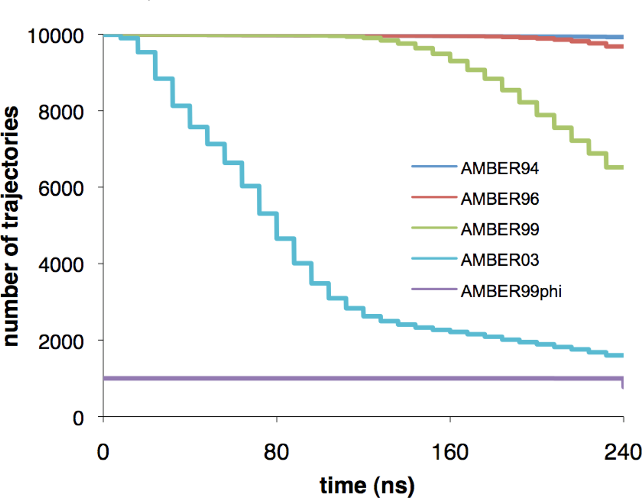
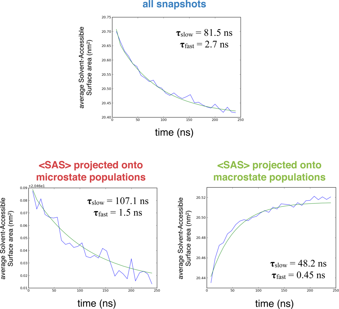
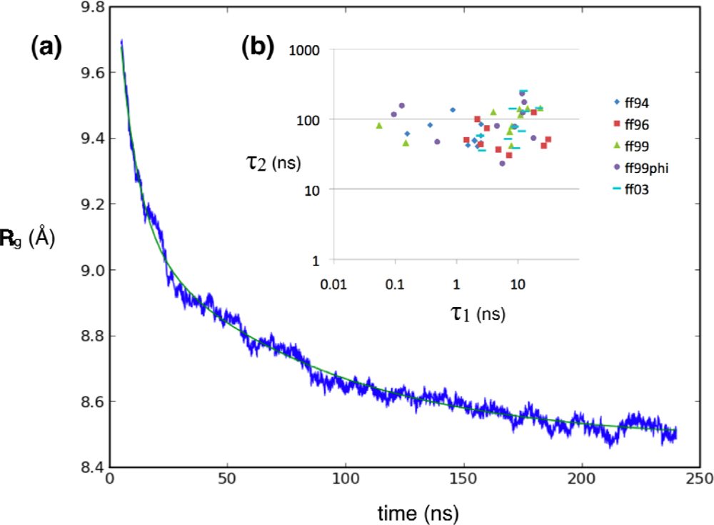
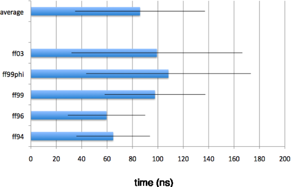
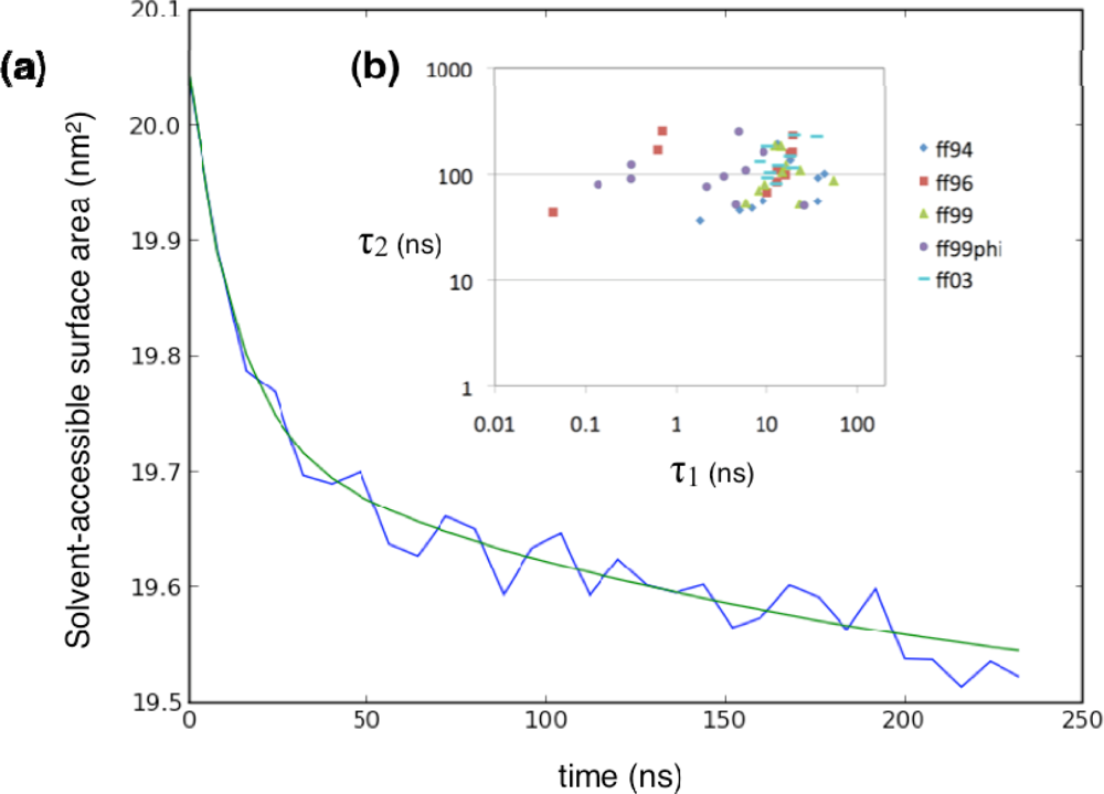
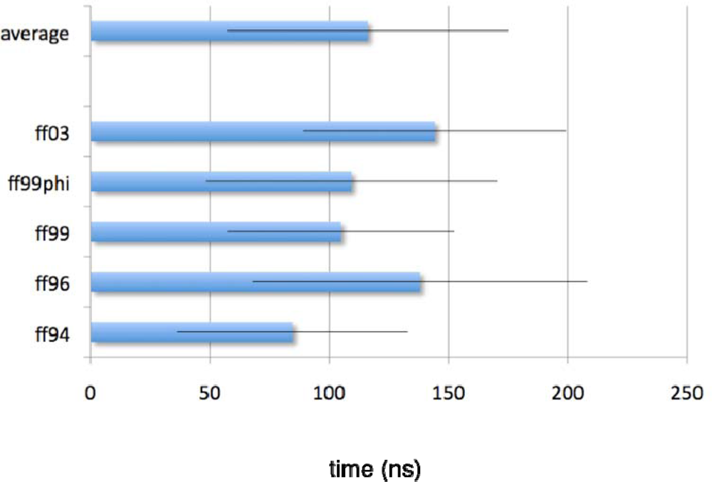
2.1. Simulated relaxation kinetics
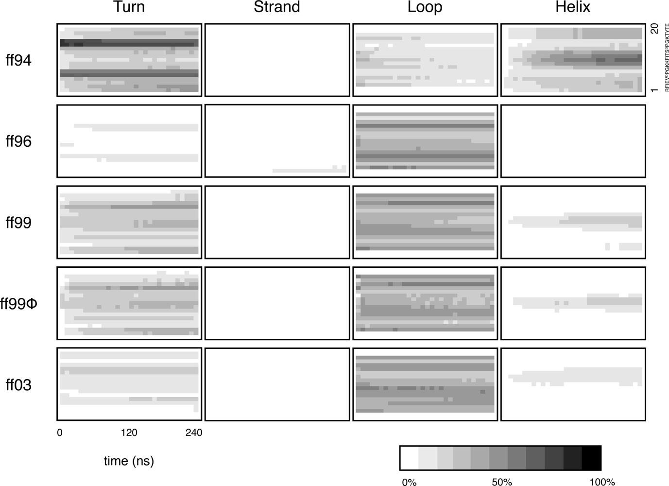
2.2. Secondary structures over time
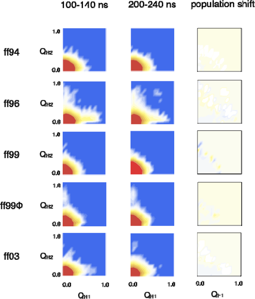
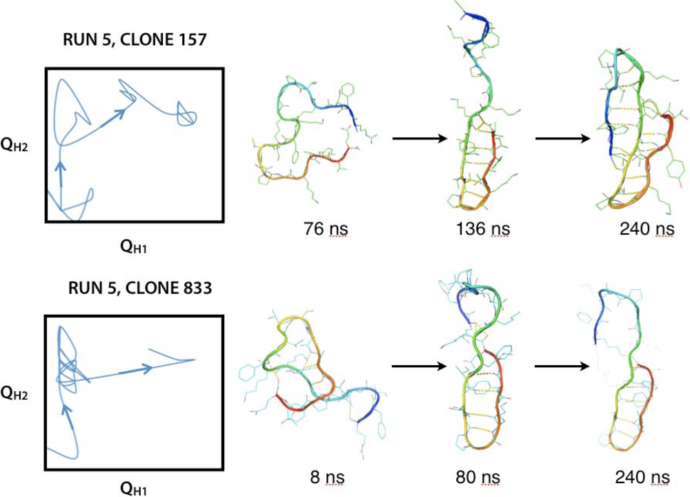
2.3. Hairpin formation over time
2.3.1. QH1 and QH2 at 100–150 ns and 200–230 ns overtime
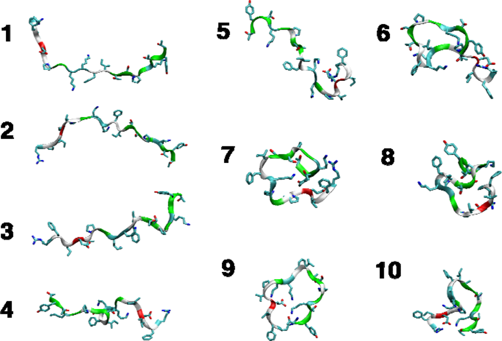
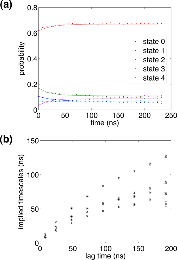
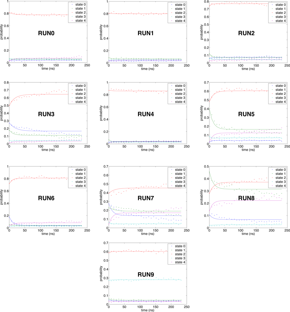
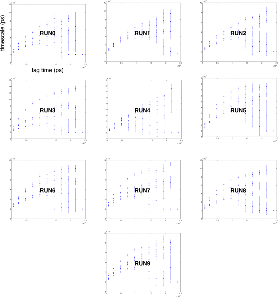
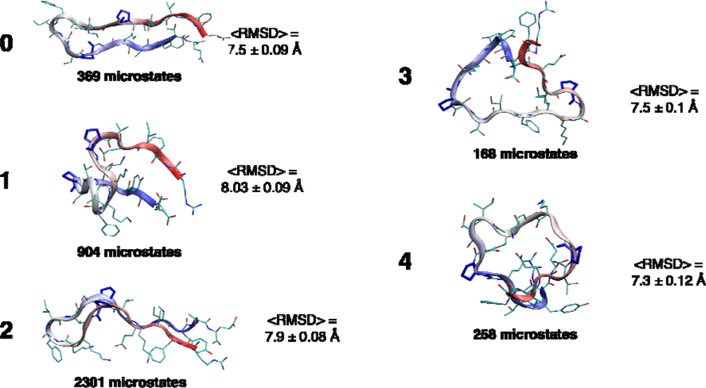
2.4. Conformational clustering and Markov State Model (MSM) analysis
3. Experimental Section
3.1. System preparation and simulation protocol
3.2. Exponential curve fitting
3.3. Secondary structure and “native” hairpin contacts
3.3. Kinetics-based clustering for building Markov State Models (MSM)
3.4. Markov State Model (MSM) construction
4. Conclusions
Supplementary Materials
Supplementary Material

| model | conf | A (Å) | B(Å) | C(Å) | τ1(ns) | τ2 (ns) | |||||
|---|---|---|---|---|---|---|---|---|---|---|---|
| ff94 | 0 | 5.033 | ± 0.345 | 0.794 | ± 0.004 | 7.795 | ± 0.001 | 2.493 | ± 0.360 | 57.757 | ±0.354 |
| l | 5.006 | 0.704 | 0.517 | 0.004 | 7.820 | 0.001 | 1.967 | 0.473 | 48.438 | 0.259 | |
| 2 | 4.950 | 0.374 | 0.461 | 0.003 | 8.147 | 0.002 | 2.507 | 0.389 | 84.182 | 0.751 | |
| 3 | 5.018 | 0.397 | 0.846 | 0.005 | 8.133 | 0.001 | 2.506 | 0.426 | 45.982 | 0.345 | |
| 4 | 4.981 | 0.744 | 1.107 | 0.007 | 8.240 | 0.001 | 2.187 | 0.623 | 40.717 | 0.362 | |
| 5 | 5.070 | 41.314 | 0.561 | 0.003 | 7.656 | 0.004 | 0.867 | 5.824 | 134.93 | 1.281 | |
| 6 | 5.014 | - | 1.404 | 0.004 | 7.948 | 0.001 | 0.157 | - | 61.837 | 0.449 | |
| 7 | 4.952 | - | 0.460 | 0.002 | 7.678 | 0.001 | 0.370 | - | 81.967 | 0.448 | |
| 8 | 5.032 | 0.693 | 0.663 | 0.004 | 7.864 | 0.001 | 1.953 | 0.460 | 49.997 | 0.282 | |
| 9 | 5.020 | 1.677 | 0.444 | 0.004 | 8.241 | 0.001 | 1.533 | 0.717 | 42.272 | 0.256 | |
| ff96 | 0 | 5.043 | 0.662 | 0.992 | 0.009 | 9.350 | 0.002 | 2.454 | 0.688 | 43.309 | 0.563 |
| 1 | 4.955 | 0.587 | 0.566 | 0.008 | 8.929 | 0.002 | 2.456 | 0.606 | 43.875 | 0.476 | |
| 2 | 4.979 | 4.446 | 0.500 | 0.006 | 9.163 | 0.002 | 1.442 | 1.670 | 50.432 | 0.543 | |
| 3 | 4.837 | 0.832 | 0.239 | 0.004 | 9.379 | 0.005 | 2.177 | 0.668 | 99.665 | 1.574 | |
| 4 | 4.807 | 0.364 | 1.074 | 0.007 | 9.697 | 0.004 | 3.115 | 0.583 | 74.105 | 1.387 | |
| 5 | −1.262 | 1.172 | 1.304 | 1.176 | 9.037 | 0.004 | 26.411 | 7.628 | 41.577 | 11.188 | |
| 6 | −1.433 | 0.108 | 1.515 | 0.019 | 8.750 | 0.001 | 4.805 | 0.474 | 36.572 | 0.632 | |
| 7 | −1.541 | 0.962 | 1.045 | 0.964 | 8.997 | 0.005 | 31.123 | 7.958 | 51.380 | 13.122 | |
| 8 | 0.550 | 0.016 | 0.400 | 0.010 | 8.444 | 0.012 | 18.133 | 0.522 | 124.259 | 5.210 | |
| 9 | 0.522 | 0.028 | 0.404 | 0.030 | 8.628 | 0.001 | 7.164 | 0.402 | 30.423 | 0.610 | |
| ff99 | 0 | 1.113 | 0.027 | 0.779 | 0.006 | 7.840 | 0.002 | 7.309 | 0.227 | 66.321 | 0.655 |
| 1 | 0.963 | 0.014 | 0.332 | 0.004 | 7.921 | 0.008 | 10.618 | 0.227 | 138.224 | 2.921 | |
| 2 | 0.771 | 0.016 | 0.561 | 0.005 | 8.095 | 0.007 | 11.026 | 0.286 | 114.416 | 2.380 | |
| 3 | 1.067 | 0.026 | 0.672 | 0.007 | 8.477 | 0.003 | 7.963 | 0.268 | 79.218 | 1.161 | |
| 4 | 1.440 | 0.014 | 0.604 | 0.006 | 8.258 | 0.013 | 14.344 | 0.403 | 141.921 | 5.159 | |
| 5 | 1.009 | - | 0.612 | 0.002 | 7.829 | 0.002 | 0.055 | - | 81.050 | 0.513 | |
| 6 | 1.096 | - | 1.305 | 0.004 | 8.079 | 0.001 | 0.149 | - | 45.977 | 0.327 | |
| 7 | −1.639 | 0.077 | 0.604 | 0.003 | 7.716 | 0.005 | 3.980 | 0.195 | 125.616 | 1.470 | |
| 8 | 1.128 | 0.022 | 0.494 | 0.014 | 7.866 | 0.001 | 7.816 | 0.279 | 41.492 | 0.485 | |
| 9 | 0.533 | 0.021 | 0.089 | 0.010 | 8.270 | 0.017 | 23.216 | 0.601 | 143.168 | 7.718 | |
| ff99ϕ | 0 | 1.020 | 0.028 | 0.630 | 0.021 | 8.386 | 0.035 | 8.861 | 0.622 | 77.890 | 14.298 |
| 1 | 1.160 | 0.029 | 0.437 | 0.017 | 7.850 | 0.030 | 12.616 | 0.599 | 174.122 | 11.908 | |
| 2 | 0.708 | 0.138 | 0.639 | 0.154 | 8.289 | 0.006 | 17.907 | 2.385 | 53.769 | 4.931 | |
| 3 | 1.388 | 0.240 | 0.942 | 0.013 | 8.387 | 0.008 | 4.552 | 0.780 | 80.028 | 2.651 | |
| 4 | 1.479 | 0.199 | 1.406 | 0.114 | 8.655 | 0.003 | 5.569 | 1.561 | 23.287 | 1.543 | |
| 5 | 0.358 | - | 0.872 | 0.006 | 7.841 | 0.008 | 0.095 | - | 116.315 | 2.487 | |
| 6 | 0.587 | 0.049 | 1.159 | 0.056 | 7.737 | 0.073 | 11.707 | 0.863 | 232.291 | 31.895 | |
| 7 | 0.497 | - | 0.437 | 0.012 | 7.852 | 0.015 | 0.128 | - | 155.409 | 4.771 | |
| 8 | 1.197 | 0.031 | 0.332 | 0.009 | 7.963 | 0.016 | 12.026 | 0.645 | 123.404 | 5.806 | |
| 9 | 0.545 | - | 0.624 | 0.008 | 8.160 | 0.003 | 0.482 | - | 47.257 | 0.713 | |
| ff03 | 0 | 1.285 | 0.027 | 0.630 | 0.011 | 8.386 | 0.006 | 8.861 | 0.381 | 77.890 | 2.070 |
| 1 | 0.931 | 0.024 | 0.533 | 0.009 | 7.943 | 0.014 | 8.203 | 0.255 | 140.234 | 4.637 | |
| 2 | 0.583 | 0.015 | 0.218 | 0.008 | 8.442 | 0.018 | 13.182 | 0.433 | 128.283 | 6.417 | |
| 3 | 0.382 | 0.016 | 0.825 | 0.057 | 8.213 | 0.068 | 12.315 | 0.392 | 251.316 | 29.238 | |
| 4 | 1.795 | 0.049 | 0.839 | 0.018 | 8.550 | 0.004 | 6.876 | 0.450 | 52.116 | 1.267 | |
| 5 | 0.657 | 0.356 | 0.361 | 0.005 | 8.190 | 0.003 | 2.423 | 0.369 | 58.054 | 0.680 | |
| 6 | 0.834 | 0.044 | 0.664 | 0.019 | 8.273 | 0.042 | 22.166 | 1.213 | 143.512 | 17.958 | |
| 7 | −0.681 | 0.026 | 0.352 | 0.033 | 8.085 | 0.002 | 9.314 | 0.451 | 38.338 | 1.003 | |
| 8 | 0.525 | 0.019 | 0.833 | 0.020 | 8.202 | 0.005 | 11.543 | 0.452 | 67.408 | 1.962 | |
| 9 | 0.448 | 0.275 | 0.571 | 0.008 | 8.487 | 0.002 | 2.592 | 0.343 | 35.544 | 0.396 | |
| model | conf | A (nm2) | B (nm2) | C (nm2) | τ1(ns) | τ2 (ns) | |||||||
|---|---|---|---|---|---|---|---|---|---|---|---|---|---|
| ff94 | 0 | 0.314 | ±0.06 | 0.263 | ±0.101 | 19.46 | ± 0.147 | 13.20 | ±1.22 | 191.22 | ±57.71 | ||
| 1 | 0.127 | 0.06 | 0.422 | 0.054 | 19.50 | 0.008 | 1.85 | 1.44 | 36.41 | 2.56 | |||
| 2 | 0.135 | 1.64 | 0.242 | 1.525 | 19.56 | 0.135 | 36.17 | 25.43 | 92.36 | 105.64 | |||
| 3 | 0.127 | 0.09 | 0.281 | 0.084 | 19.22 | 0.015 | 9.12 | 1.18 | 55.98 | 5.99 | |||
| 4 | 0.220 | 0.12 | 0.382 | 0.051 | 19.90 | 0.105 | 18.18 | 2.49 | 135.26 | 42.12 | |||
| 5 | −0.133 | 0.10 | −0.093 | 0.073 | 19.78 | 0.033 | 12.73 | 1.72 | 84.80 | 12.77 | |||
| 6 | 0.496 | 2.15 | 0.078 | 1.999 | 19.75 | 0.162 | 42.56 | 34.48 | 101.07 | 140.83 | |||
| 7 | 0.149 | 9.51 | −0.145 | 9.481 | 19.33 | 0.047 | 35.93 | 72.40 | 55.47 | 125.59 | |||
| 8 | 0.078 | 0.09 | 0.253 | 0.076 | 19.42 | 0.012 | 6.75 | 0.90 | 47.88 | 4.59 | |||
| 9 | 0.135 | 0.08 | 0.218 | 0.064 | 19.52 | 0.011 | 4.96 | 0.81 | 45.57 | 3.79 | |||
| ff96 | 0 | 0.112 | 0.10 | 0.638 | 0.084 | 20.46 | 0.025 | 10.10 | 1.41 | 67.55 | 9.27 | ||
| 1 | 0.270 | 0.10 | 0.541 | 0.054 | 20.28 | 0.069 | 13.07 | 1.82 | 110.48 | 25.30 | |||
| 2 | 0.265 | 0.14 | 0.442 | 0.075 | 20.16 | 0.179 | 18.05 | 3.11 | 155.05 | 71.44 | |||
| 3 | 0.268 | 0.15 | −0.314 | 0.082 | 20.56 | 0.201 | 19.13 | 3.39 | 160.73 | 82.07 | |||
| 4 | 0.032 | 0.03 | 0.756 | 0.078 | 20.81 | 0.095 | 0.62 | - | 168.33 | 30.95 | |||
| 5 | −0.408 | 0.16 | 0.139 | 0.108 | 20.54 | 0.066 | 16.06 | 2.90 | 98.79 | 26.95 | |||
| 6 | −0.203 | 0.06 | 0.301 | 0.048 | 20.71 | 0.010 | 0.04 | - | 43.51 | 3.10 | |||
| 7 | −0.199 | 0.14 | −0.451 | 0.103 | 20.29 | 0.047 | 12.97 | 2.28 | 84.86 | 18.38 | |||
| 8 | 0.412 | 0.12 | 0.215 | 0.286 | 19.91 | 0.399 | 19.35 | 3.04 | 233.22 | 178.51 | |||
| 9 | 0.043 | 0.05 | 0.523 | 0.221 | 19.91 | 0.242 | 0.70 | - | 258.40 | 98.31 | |||
| ff99 | 0 | 0.153 | 0.07 | 0.423 | 0.057 | 19.90 | 0.014 | 5.79 | 0.74 | 53.42 | 4.59 | ||
| 1 | 0.311 | 0.08 | 0.404 | 0.059 | 19.72 | 0.032 | 9.57 | 1.26 | 79.88 | 11.15 | |||
| 2 | 0.272 | 0.09 | 0.340 | 0.067 | 19.79 | 0.027 | 8.08 | 1.18 | 70.72 | 9.35 | |||
| 3 | 0.187 | 0.06 | 0.577 | 0.098 | 19.64 | 0.144 | 12.41 | 1.21 | 185.05 | 55.65 | |||
| 4 | 0.355 | 0.08 | 0.482 | 0.111 | 19.97 | 0.172 | 14.40 | 1.62 | 183.55 | 67.44 | |||
| 5 | −0.301 | 1.18 | 0.330 | 1.162 | 19.83 | 0.028 | 22.91 | 12.15 | 52.47 | 29.19 | |||
| 6 | 0.306 | 15.03 | 0.421 | 14.842 | 20.03 | 0.204 | 53.59 | 174.55 | 87.42 | 398.29 | |||
| 7 | 0.084 | 0.29 | 0.065 | 0.205 | 19.58 | 0.102 | 23.27 | 5.61 | 109.14 | 47.79 | |||
| 8 | 0.262 | 0.11 | 0.173 | 0.068 | 19.89 | 0.061 | 14.83 | 2.11 | 105.48 | 23.74 | |||
| 9 | 0.309 | 0.13 | 0.445 | 0.062 | 19.82 | 0.093 | 16.30 | 2.56 | 121.68 | 36.46 | |||
| ff99ϕ | 0 | 0.691 | 0.39 | 0.444 | 0.008 | 19.92 | 0.010 | 3.35 | 0.72 | 95.62 | 3.01 | ||
| 1 | 1.018 | 0.21 | 0.758 | 0.022 | 19.80 | 0.005 | 4.52 | 0.78 | 51.41 | 1.65 | |||
| 2 | 1.599 | 0.99 | −0.574 | 0.997 | 20.00 | 0.012 | 25.66 | 9.87 | 50.49 | 18.24 | |||
| 3 | 0.601 | 1.39 | 0.681 | 0.009 | 19.85 | 0.007 | 2.18 | 1.14 | 76.76 | 1.99 | |||
| 4 | 0.985 | 0.13 | 0.461 | 0.011 | 20.23 | 0.016 | 5.78 | 0.67 | 108.88 | 5.16 | |||
| 5 | 0.522 | - | 0.188 | 0.009 | 19.80 | 0.008 | 0.14 | - | 80.45 | 2.28 | |||
| 6 | 0.520 | - | 0.919 | 0.011 | 19.99 | 0.014 | 0.32 | - | 123.03 | 4.24 | |||
| 7 | 0.511 | - | 0.196 | 0.008 | 19.65 | 0.009 | 0.32 | - | 90.98 | 2.56 | |||
| 8 | 0.567 | 0.19 | 0.339 | 0.068 | 19.91 | 0.076 | 4.86 | 0.67 | 255.40 | 31.96 | |||
| 9 | 0.587 | 0.06 | 0.520 | 0.025 | 19.91 | 0.040 | 9.23 | 0.80 | 160.88 | 14.86 | |||
| ffO3 | 0 | 0.402 | 0.11 | 0.372 | 0.056 | 19.74 | 0.134 | 18.01 | 2.42 | 147.19 | 52.60 | ||
| 1 | 0.413 | 0.06 | 0.435 | 0.112 | 19.53 | 0.153 | 10.09 | 1.04 | 181.95 | 55.88 | |||
| 2 | 0.279 | 0.14 | 0.579 | 0.345 | 19.35 | 0.474 | 20.10 | 3.35 | 237.59 | 212.92 | |||
| 3 | 0.134 | 0.09 | 0.294 | 0.044 | 19.50 | 0.080 | 13.43 | 1.60 | 120.90 | 28.45 | |||
| 4 | 0.159 | 0.07 | 0.653 | 0.047 | 19.97 | 0.042 | 10.26 | 1.19 | 92.81 | 14.30 | |||
| 5 | −0.121 | 0.06 | −0.047 | 0.047 | 19.77 | 0.079 | 8.39 | 1.04 | 131.58 | 26.29 | |||
| 6 | 0.169 | 0.45 | 0.626 | 0.346 | 19.70 | 0.775 | 35.17 | 11.06 | 230.31 | 399.18 | |||
| 7 | −0.127 | 0.20 | −0.154 | 0.114 | 19.54 | 0.108 | 19.30 | 3.82 | 114.75 | 44.76 | |||
| 8 | 0.163 | 0.12 | 0.313 | 0.091 | 19.55 | 0.039 | 12.76 | 1.95 | 81.74 | 15.11 | |||
| 9 | 0.141 | 0.08 | −0.012 | 0.048 | 19.48 | 0.057 | 10.94 | 1.45 | 103.82 | 19.78 | |||
Acknowledgments
References and Notes
- Xu, Y; Purkayastha, P; Gai, F. Nanosecond folding dynamics of a three-stranded beta-sheet. J. Am. Chem. Soc 2006, 128, 15836–15842. [Google Scholar]
- Espinosa, JF; Syud, F; Gellman, S. Analysis of the factors that stabilize a designed two-stranded antiparallel β-sheet. Protein Sci 2002, 77, 1492–1505. [Google Scholar]
- Stanger, H; Gellman, SH. Rules for antiparallel β-sheet design: D-Pro-Gly is superior to L-Asn-Gly for β-hairpin nucleation. J. Am. Chem. Soc 1998, 120, 4236–4237. [Google Scholar]
- Schenck, H; Gellman, SH. Use of a designed triple-stranded antiparallel β-sheet to probe β-sheet cooperativity in aqueous solution. J. Am. Chem. Soc 1998, 120, 4869–4870. [Google Scholar]
- Syud, F; Stanger, H; Mortell, H.S; Espinosa, J.F; Fisk, J.D; Fry, C.G; Gellman, S.H. Influence of strand number on antiparallel beta-sheet stability in designed three- and four-stranded beta-sheets. J. Mol. Biol 2003, 326, 553–568. [Google Scholar]
- Arora, P; Oas, T; Myers, J. Fast and faster: A designed variant of the B-domain of protein A folds in 3 microsec. Protein Sci 2004, 13, 847–853. [Google Scholar]
- Kubelka, J; Chiu, T; Davies, D; Eaton, W; Hofrichter, J. Sub-microsecond protein folding. J. Mol. Biol 2006, 359, 546–553. [Google Scholar]
- Yang, W; Gruebele, M. Folding λ-Repressor at Its Speed Limit. Biophys. J 2004, 87, 596–608. [Google Scholar]
- Ensign, D; Kasson, P; Pande, V. Heterogeneity Even at the Speed Limit of Folding: Large-scale Molecular Dynamics Study of a Fast-folding Variant of the Villin Headpiece. J. Mol. Biol 2007, 374, 806–816. [Google Scholar]
- Kubelka, J; Hofrichter, J; Eaton, WA. The protein folding ‘speed limit’. Curr. Opin. Struct. Biol 2004, 14, 76–88. [Google Scholar]
- Eaton, WA; Muñoz, V; Thompson, PA; Henry, ER. Kinetics and Dynamics of Loops, Alpha-Helices, Beta-Hairpins, and Fast-Folding Proteins. Acc. Chem. Res 1998, 31, 745–753. [Google Scholar]
- Ghosh, K; Ozkan, SB; Dill, KA. The ultimate speed limit to protein folding is conformational searching. J. Am. Chem. Soc 2007, 129, 11920–11927. [Google Scholar]
- Deechongkit, S; Nguyen, H; Jager, M; Powers, E; Gruebele, M; Kelly, JW. β-Sheet folding mechanisms from perturbation energetics. Curr. Opin. Struct. Biol 2006, 16, 94–101. [Google Scholar]
- Xu, Y; Bunagan, MR; Tang, J; Gai, F. Probing the Kinetic Cooperativity of β-Sheet Folding Perpendicular to the Strand Direction. Biochemistry 2008, 47, 2064–2070. [Google Scholar]
- Gruebele, M. Comment on probe-dependent and nonexponential relaxation kinetics: Unreliable signatures of downhill protein folding. Proteins 2008, 70, 1099–1102. [Google Scholar]
- Liu, F; Gruebele, M. Downhill dynamics and the molecular rate of protein folding. Chem. Phys. Lett 2008, 461, 1–8. [Google Scholar]
- Smith, A; Tokmakoff, A. Probing local structural events in β-hairpin unfolding with transient nonlinear infrared spectroscopy. Angew. Chem. Int. Ed 2007, 46, 7984–7987. [Google Scholar]
- Wang, H; Sung, S. Molecular dynamics simulations of three-strand β-sheet folding. J. Am. Chem. Soc 2000, 122, 1999–2009. [Google Scholar]
- Roe, DR; Hornak, V; Simmerling, C. Folding cooperativity in a three-stranded β-sheet model. J. Mol. Biol 2005, 352, 370–381. [Google Scholar]
- Kuznetsov, SV; Hilario, J; Keiderling, T.A; Ansari, A. Spectroscopic studies of structural changes in two-sheet-forming peptides show an ensemble of structures that unfold noncooperatively. Biochemistry 2003, 42, 4321–4332. [Google Scholar]
- Shirts, MR; Pande, VS. Screen savers of the world, unite! Science 2000, 290, 1903–1904.
- Lindahl, E; Hess, B; van der Spoel, D. GROMACS 3.0: A package for molecular simulation and trajectory analysis. J. Mol. Model 2001, 7, 306–317. [Google Scholar]
- Cornell, WD; Cieplak, P; Bayly, CI; Gould, IR; Merz, K.M, Jr; Ferguson, D.M; Spellmeyer, D.C; Fox, T; Caldwell, JW; Kollman, P.A. A second generation force field for the simulation of proteins nucleic acids and organic molecules. J. Am. Chem. Soc 1995, 117, 5179–5197. [Google Scholar]
- Kollman, P; Dixon, R; Cornell, W; Fox, T; Chipot, C; Pohorille, A. The development/application of a “minimalist” organic/biochemical molecular mechanic force field using a combination of ab initio calculations and experimental data. In Computer Simulations of Biomolecular Systems: Theoretical and Experimental Applications; van Gunsteren, WF, Wiener, PK, Eds.; Escom: Dordrecht, The Netherlands, 1997; pp. 83–96. [Google Scholar]
- Wang, J; Cieplak, P; Kollman, P.A. How well does a restrained electrostatic potential (RESP) model perform in calculating conformational energies of organic and biological molecules? J. Comput. Chem 2000, 21, 1049–1074. [Google Scholar]
- Sorin, EJ; Pande, VS. Exploring the helix-coil transition via all-atom equilibrium ensemble simulations. Biophys. J 2005, 88, 2472–2493. [Google Scholar]
- Duan, Y; Wu, C; Chowdhury, S; Lee, M.L; Xiong, G. A point-charge force field for molecular mechanics simulations of proteins based on condensed-phase quantum mechanical calculations. J. Comp. Chem 2003, 24, 1999–2012. [Google Scholar]
- Best, RB; Hummer, G. Reaction coordinates and rates from transition paths. Proc. Natl. Acad. Sci 2005, 102, 6732–6737. [Google Scholar]
- Juraszek, J; Bolhuis, P. Rate constant and reaction coordinate of Trp-Cage folding in explicit water. Biophys. J 2008, 95, 4246–4257. [Google Scholar]
- Walsh, STR; Cheng, RP; Wright, WW; Alonso, DOV; Daggett, V; Vanderkooi, JM; DeGrado, WF. The hydration of amides in helices; a comprehensive picture from molecular dynamics, IR, and NMR. Protein. Sci 2003, 12, 520–531. [Google Scholar]
- Snow, C; Sorin, E; Rhee, Y; Pande, V. How well can simulation predict protein folding kinetics and thermodynamics? Annu. Rev. Biophys. Biomol. Struct 2005, 34, 43–69. [Google Scholar]
- Jorgensen, WL; Chandrasekhar, J; Madura, JD; Impey, RW; Klein, ML. Comparison of simple potential functions for simulating liquid water. J. Chem. Phys 1983, 79, 926. [Google Scholar]
- Kabsch, W; Sander, C. Dictionary of protein secondary structure: pattern recognition of hydrogen-bonded and geometrical features. Biopolymers 1983, 22, 2577–2637. [Google Scholar]
- Shirts, MR; Pande, VS. Mathematical analysis of coupled parallel simulations. Phys. Rev. Lett 2001, 86, 4983–4987. [Google Scholar]
- Marianayagam, N; Fawzi, NL; Head-Gordon, T. Protein folding by distributed computing and the denatured state ensemble. Proc. Natl. Acad. Sci. USA 2005, 102, 16684–16689. [Google Scholar]
- Colombo, G; Roccatano, D; Mark, AE. Folding and stability of the three-stranded beta-sheet peptide betanova: Insights from molecular dynamics simulations. Prot. Struct. Func. Genet 2002, 46, 380–392. [Google Scholar]
- Macias, MJ; Gervais, V; Civera, C; Oschkinat, H. Structural analysis of WW domains and design of a WW prototype. Nat. Struct. Biol 2000, 7, 375–379. [Google Scholar]
- Chodera, JD; Singhal, N; Pande, VS; Dill, KA; Swope, WC. Automatic discovery of metastable states for the construction of Markov models of macromolecular conformational dynamics. J. Chem. Phys 2007, 126, 155101. [Google Scholar]
- Noe, F; Fischer, S. Transition networks for modeling the kinetics of conformational change in macromolecules. Curr. Opin. Struct. Biol 2008, 8, 154–162. [Google Scholar]
- Chodera, JD; Swope, WC; Pitera, JW; Dill, K.A. Long-time protein folding dynamics from short-time molecular dynamics simulations. Multiscale Model. Sim 2006, 5, 1214–1226. [Google Scholar]
- Bates, DM; Watts, DG. Nonlinear Regression Analysis and Its Applications; Wiley: New York, 1988. [Google Scholar]
- Bowman, GR; Huang, X; Pande, VS. Using generalized ensemble simulations and Markov state models to identify conformational states. Methods, 2009; in press.
- Dasgupta, S; Long, PM. Performance guarantees for hierarchical clustering. J. Comp. Sys. Sci 2005, 70, 555–569. [Google Scholar]
- Deuflhard, P. Identification of almost invariant aggregates in reversible nearly uncoupled Markov chains. Lin. Alg. Appl 2000, 315, 39–59. [Google Scholar]
- Deuflhard, P; Weber, M. Robust Perron cluster analysis in conformation dynamics. Lin. Alg. Appl 2005, 398, 161–184. [Google Scholar]


© 2009 by the authors; licensee Molecular Diversity Preservation International, Basel, Switzerland. This article is an open-access article distributed under the terms and conditions of the Creative Commons Attribution license ( http://creativecommons.org/licenses/by/3.0/). This article is an open-access article distributed under the terms and conditions of the Creative Commons Attribution license ( http://creativecommons.org/licenses/by/3.0/).
Share and Cite
Voelz, V.A.; Luttmann, E.; Bowman, G.R.; Pande, V.S. Probing the Nanosecond Dynamics of a Designed Three-Stranded Beta-Sheet with a Massively Parallel Molecular Dynamics Simulation. Int. J. Mol. Sci. 2009, 10, 1013-1030. https://doi.org/10.3390/ijms10031013
Voelz VA, Luttmann E, Bowman GR, Pande VS. Probing the Nanosecond Dynamics of a Designed Three-Stranded Beta-Sheet with a Massively Parallel Molecular Dynamics Simulation. International Journal of Molecular Sciences. 2009; 10(3):1013-1030. https://doi.org/10.3390/ijms10031013
Chicago/Turabian StyleVoelz, Vincent A., Edgar Luttmann, Gregory R. Bowman, and Vijay S. Pande. 2009. "Probing the Nanosecond Dynamics of a Designed Three-Stranded Beta-Sheet with a Massively Parallel Molecular Dynamics Simulation" International Journal of Molecular Sciences 10, no. 3: 1013-1030. https://doi.org/10.3390/ijms10031013