Introduction
The synthesis of polynuclear coordination complexes showing magnetic properties has been an area of intensive research for many years,[
1] whose interest has recently increased due to the properties of single-molecule-magnet exhibited by some of these complexes [
2]. However, the rational design of this class of molecular materials still presents difficulties, some associated with the control of their synthesis, and others with a limited understanding of the magnetic exchange process.
In this work we present a full analysis of the magnetism of the [Cu
4(bpy)
4L
2(H
2O)
3](ClO
4)
4·2.5H
2O (bpy = bipyridine, L = aspartate) crystal [
3], a prototypical polynuclear coordination complex. Our aim is to complete an initial report on this crystal [
3], which was mainly addressed to defining its magnetic structure in order to adequately fit the experimental magnetic susceptibility curve. Here, we will apply our recently proposed first principles
bottom-up approach [
4] to the study of this crystal, thus allowing a full understanding of its magnetic properties. This is the first time we apply such methodology to crystals of polynuclear coordination complexes whose magnetic interactions are of a through-bond nature, although it has been previously shown to give appropriate descriptions of the magnetism in purely organic molecular crystals [
5] and in metal containing crystals where the magnetic interaction is through-space [
5]. The [Cu
4(bpy)
4(aspartate)
2(H
2O)
3](ClO
4)
4·2.5H
2O crystal [
3] has a structure characterized by the presence of two inequivalent, positively-charged tetranuclear Cu
II clusters per unit cell (
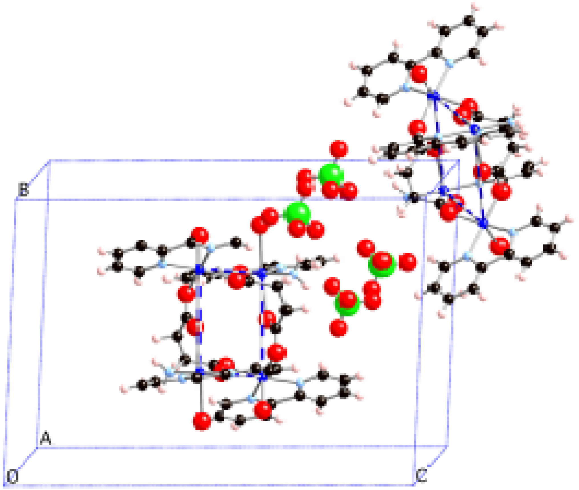
Figure 1).
Figure 1.
Packing of the [Cu4(bpy)4L2(H2O)3](ClO4)4·2.5H2O (bpy = bipyridine, L = aspartate) crystal.
Figure 1.
Packing of the [Cu4(bpy)4L2(H2O)3](ClO4)4·2.5H2O (bpy = bipyridine, L = aspartate) crystal.
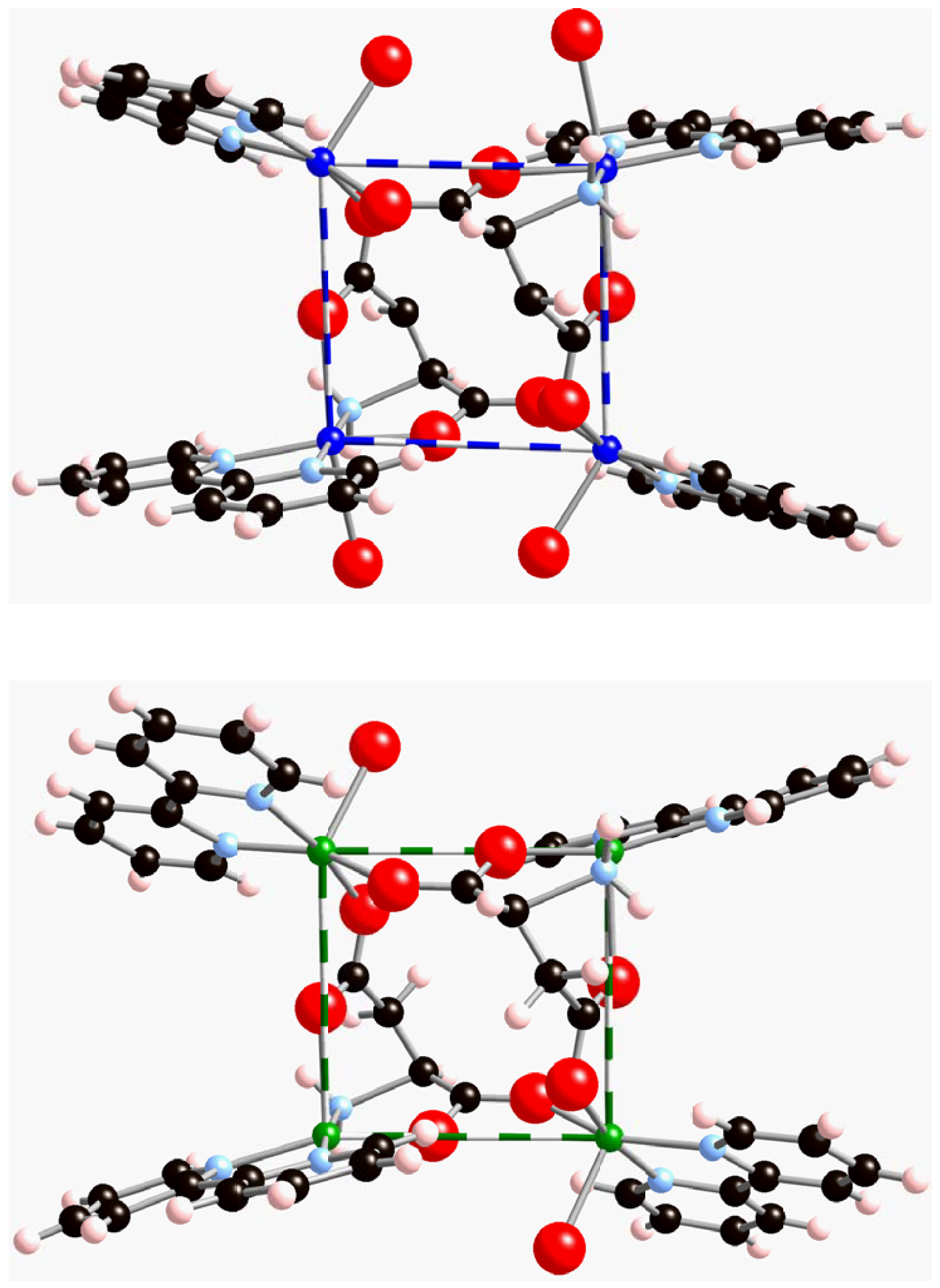
Figure 2.
View of the two non-equivalent Cu
II tetramers. The Cu
…Cu distances are given in
Table 1.
Figure 2.
View of the two non-equivalent Cu
II tetramers. The Cu
…Cu distances are given in
Table 1.
Thus, there are two types of Cu
II clusters, whose geometries differ only in very small details (
Figure 2a-b). Such tetranuclear Cu
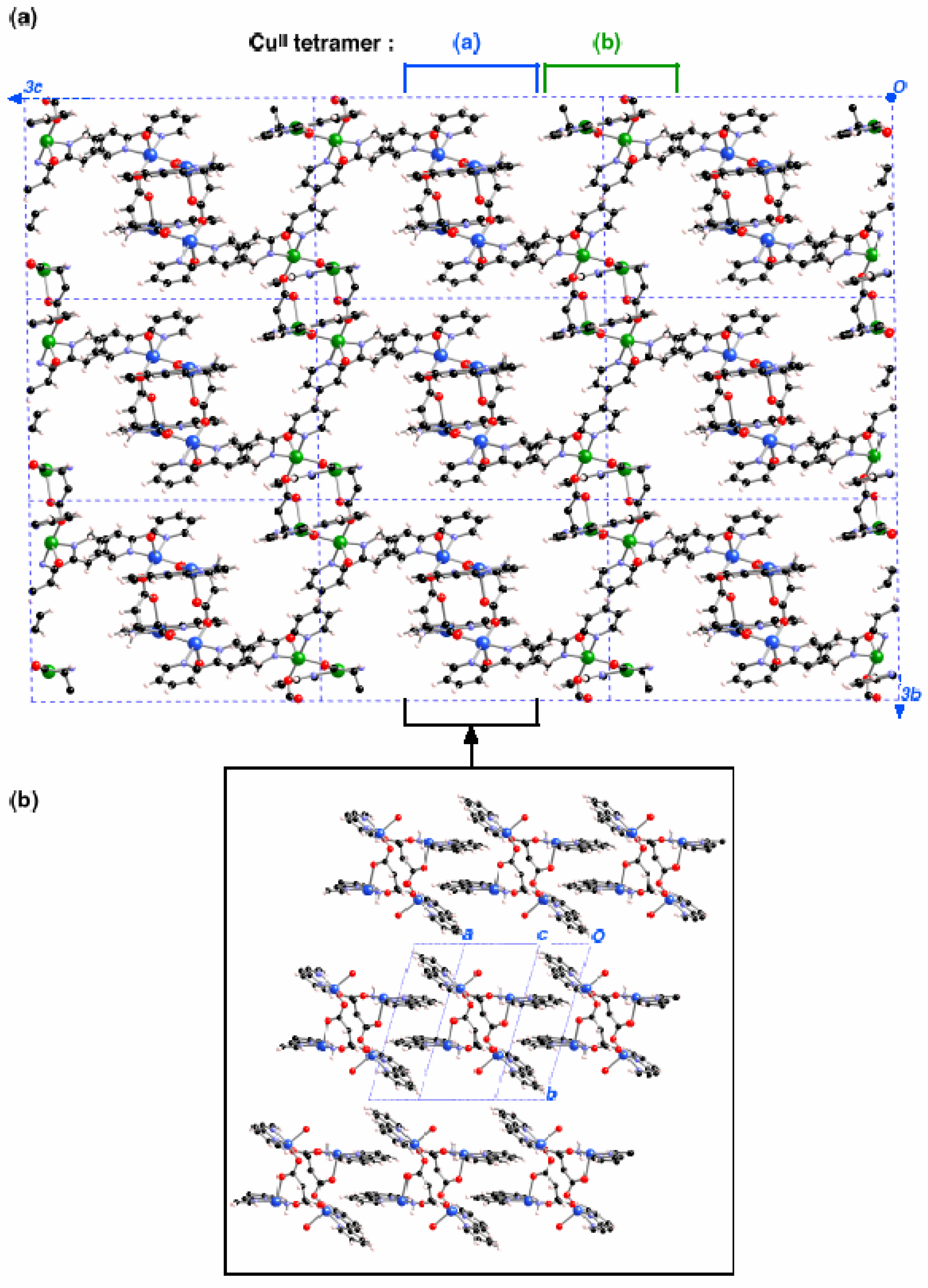
II clusters form planes along the
bc crystallographic directions (
Figure 3a, notice that non-equivalent Cu
II clusters have different colour and counterions are omitted for clarity). The shortest distances between any two Cu
II clusters take place along the
a-axis through a π
…π stacking interaction connecting bpy ligands from two equivalent clusters at 7.363Å (
Figure 3b). This fact suggested [
3] that each Cu
II cluster could be considered to be magnetically isolated.
Figure 3.
Packing of the [Cu4(bpy)4(aspartate)2(H2O)3](ClO4)4·2.5H2O crystal. (a) view of the bc plane (the two non-equivalent tetramers are identified by using blue or green color for the CuII atoms); (b) view along the a-axis of the packing for the region of (a) indicated in brackets.
Figure 3.
Packing of the [Cu4(bpy)4(aspartate)2(H2O)3](ClO4)4·2.5H2O crystal. (a) view of the bc plane (the two non-equivalent tetramers are identified by using blue or green color for the CuII atoms); (b) view along the a-axis of the packing for the region of (a) indicated in brackets.
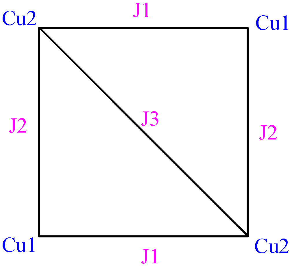
Among various possible models of magnetic interactions, preliminary
ab initio calculations indicated that the best model to describe the magnetism within the clusters was a square with three different
J magnetic interactions, as shown in
Figure 4. Given the similar geometry of the two non-equivalent Cu
II clusters, both types of clusters were supposed to fulfil the same model with the same set of
J pair interaction values. With this model, the fitting of the experimental magnetic susceptibility curve of this crystal (using a Hamiltonian
H = -Σ Jij Si Sj) gave as best
Jij parameters [
6] +8.38, -1.27 and -0.5 cm
-1. These values are similar to the microscopic
JAB pair-parameters, +11.4, -3.8 and -1.5 cm
-1, computed for one of the tetranuclear Cu
II clusters.
Figure 4.
Schematic view of the magnetic structure for each CuII tetranuclear compound
Figure 4.
Schematic view of the magnetic structure for each CuII tetranuclear compound
Our first-principles bottom-up analysis of this crystal begins by computing the microscopic JAB pair interactions between all unique spin-containing metal centers present in the crystal. From these values, we define the magnetic structure of the crystal. Once this is done, our approach defines a finite model of that magnetic structure, which is used to compute the eigenvalues of the Heisenberg Hamiltonian. These eigenvalues are then used to compute the desired macroscopic magnetic properties, in general the magnetic susceptibility curve. The key contribution of this method is that it connects the macroscopic behaviour with the microscopic JAB values in a rigorous quantitative form, thus allowing the correlation of the macroscopic behaviour with the geometry of the radical centres. This is the first time we apply our approach for a metal-containing system where the interactions are mainly through-bond. We will show that the numerically simulated χT(T) curve follows the same pattern as the experimental data, although it also presents some differences. Possible reasons for this discrepancy will be discussed.
Methodology
The basic idea of our
bottom-up approach consists on determining the magnetic structure of the crystal on the basis of the values of the microscopic
JAB pair-interactions between the radicals of the crystal, and then to use such microscopic data to quantitatively compute the macroscopic magnetic properties (for instance, the magnetic susceptibility). Such connection can be achieved by building a Heisenberg Hamiltonian (equation 1) that describes the magnetic structure of the studied crystal:
being the spin operator associated with the radical
A, and
the identity operator. The magnetic interactions present in the crystal are quantitatively reproduced in the Heisenberg Hamiltonian (1) once the magnitude of the microscopic magnetic interaction
JAB is introduced
for each unique AB radical-radical pair (see below). In order to extrapolate the methodology developed for purely-organic molecular magnets to polynuclear coordination complexes containing open-shell metals, it is enough to replace the organic radicals by the spin-containing metals (in the study case here, the Cu
II atoms) and compute the microscopic magnetic interaction
JAB using the Cu
II-(bridging-ligand)-Cu
II entity (by bridging-ligand we indicate the ligand of the polynuclear coordination complex that acts as a through-bond link between two Cu
II metals).
This procedure is non-biased and quantitatively accurate, once one takes the precaution of enforcing that we include in the JAB evaluation all the unique first-nearest neighbours pairs of through-bond connected spin-containing metal centres and the most important second-nearest neighbours. Notice that the form of the Heisenberg Hamiltonian (1) is related with the more usual one by a shift in the scale of energies. We will use equation (1) here because it is easier to implement in our programs. Once (1) has been defined in quantitative terms, it enables us to obtain the energy spectrum. From this spectrum, using Statistical Mechanics, one can compute the macroscopic magnetic properties at any given temperature (e.g. the magnetic susceptibility and heat capacity, the two macroscopic magnetic properties most commonly employed in experimental magnetic studies of crystals). The process is first principles, since it makes no assumption on the result, and bottom-up, as begins at the microscopic level and goes to the macroscopic.
The practical implementation of this first principles
bottom-up approach consists in the following sequential steps:
- (1)
A detailed analysis of the crystal packing to identify, in an unbiased and systematic way, all unique relevant AB pairs of spin-containing metal centres. We will deliberately select more pairs than the first nearest neighbours, which are the usual candidates in the literature.
- (2)
The ab initio computation of the JAB magnetic interactions for all selected pairs of spin-containing metal centres (in our case, the two CuII atoms and the ligands that connect them by through-bond magnetic interactions). JAB is obtained by computing the singlet-triplet energy difference using ab initio methods (in our case, using the B3LYP density functional, as we indicate hereafter).
- (3)
Determination of the magnetic structure of the crystal, by inspection of the JAB values for each pair of spin-containing metal centres and the topological connections they make. Each spin-containing metal centre can be seen as a radical site, connected to another when |JAB | is larger than a given threshold (estimated as |0.05| cm-1 in our calculations). Then, one searches for the (finite-sized) minimal magnetic model space that describes the magnetic structure of the crystal in an even way. The set of spin-containing metal centres of the minimal magnetic model space defines a spin space. This is the spin space used to compute the matrix representation of the Heisenberg Hamiltonian (1). The JAB parameters required in that representation are those computed in step 2.
- (4)
As a final step, the Heisenberg Hamiltonian matrix is diagonalised and its eigenvalues are obtained. That set of energies (the energy spectrum) is used to compute the magnetic susceptibility χ(T) and/or heat capacity Cp(T) using standard statistical mechanics.
The size (N) of the minimal magnetic model space must be small enough to keep the size of the Heisenberg Hamiltonian matrix as small as possible, but it must also contain all important magnetic pathways detected within the crystal in an even form. In practice, N must be not larger than 16, due to the cost of fully diagonalising the Heisenberg matrices for larger values. To test the validity of our minimal magnetic model space, we will check the convergence of our results (e.g. χ vs. T) when the model space is replicated along the crystallographic directions (if the minimal magnetic model space is properly chosen, the χ(T) results should converge rapidly among extended models to the χ(T) data obtained with the minimal model, which should approach the experimental χ(T) value). From our experience, the most essential issue in our procedure is the selection of a proper subset of the magnetic topology of the crystal.
As already mentioned, the only information required to compute the matrix of the Heisenberg operator are the values of the microscopic
JAB pair interactions. They are computed using
ab initio methods from the energy difference between the high and low spin states of the pair of radicals. In the case of the Cu
II-ligand-Cu
II entities, the value of
JAB for any pair is obtained by subtracting the energy of the most stable open-shell singlet (OSS) and triplet (T) states at the pair geometry, using the broken-symmetry approximation [
7] to compute the energy of the OSS state (that is,
JAB = E(BS-OSS) - E(T)). Both energy values have been computed using the UB3LYP functional [
8] and the Ahlrichs pVDZ basis set, adding diffuse functions [
9] (a 10
-8 convergence criterion on the total energy and 10
-10 on the integrals was used to ensure enough accuracy in the computation of the
JAB parameters). Notice that the original formulation of the broken-symmetry approximation developed for the UHF method suggests that the overlap should be taken into consideration, and the
JAB should be computed according to the expression [
9]
JAB = 2(E(BS-OSS) - E(T) when there is no overlap between magnetic orbitals. However, in good agreement with other authors, [
10] we have found that the use of the
JAB = E(BS-OSS) - E(T) expression together with energies obtained using the B3LYP functional provides better results for the magnetic susceptibility curves. Such a fact has been attributed by some authors to error compensation and by others to some intrinsic behaviour of the DFT functionals [
10]. All DFT calculations were done using the Gaussian-98 package [
11].
Results and Discussion
The structure of the [Cu
4(bpy)
4(aspartate)
2(H
2O)
3](ClO
4)
4·2.5H
2O crystal can be viewed as forming planes of [Cu
4(bpy)
4(aspartate)
2(H
2O)
3]
4+ cations along the
bc-axes, which then stack along the
a axis (
Figure 3).
Figure 1 shows the two inequivalent tetranuclear Cu
II clusters, one of them is located in the centre and the other in the corner of the unit cell (Cu
II atoms coloured in blue and green in
Figure 2a/
Figure 3a and
Figure 2b/
Figure 3a, respectively). The bpy groups of one
bc-plane interlock with those of the nearby
bc-plane, so that nearby Cu
II clusters are separated by through-space bpy
…bpy interactions along the
a-axis (
Figure 3b). The packing of this crystal is driven by ionic forces.
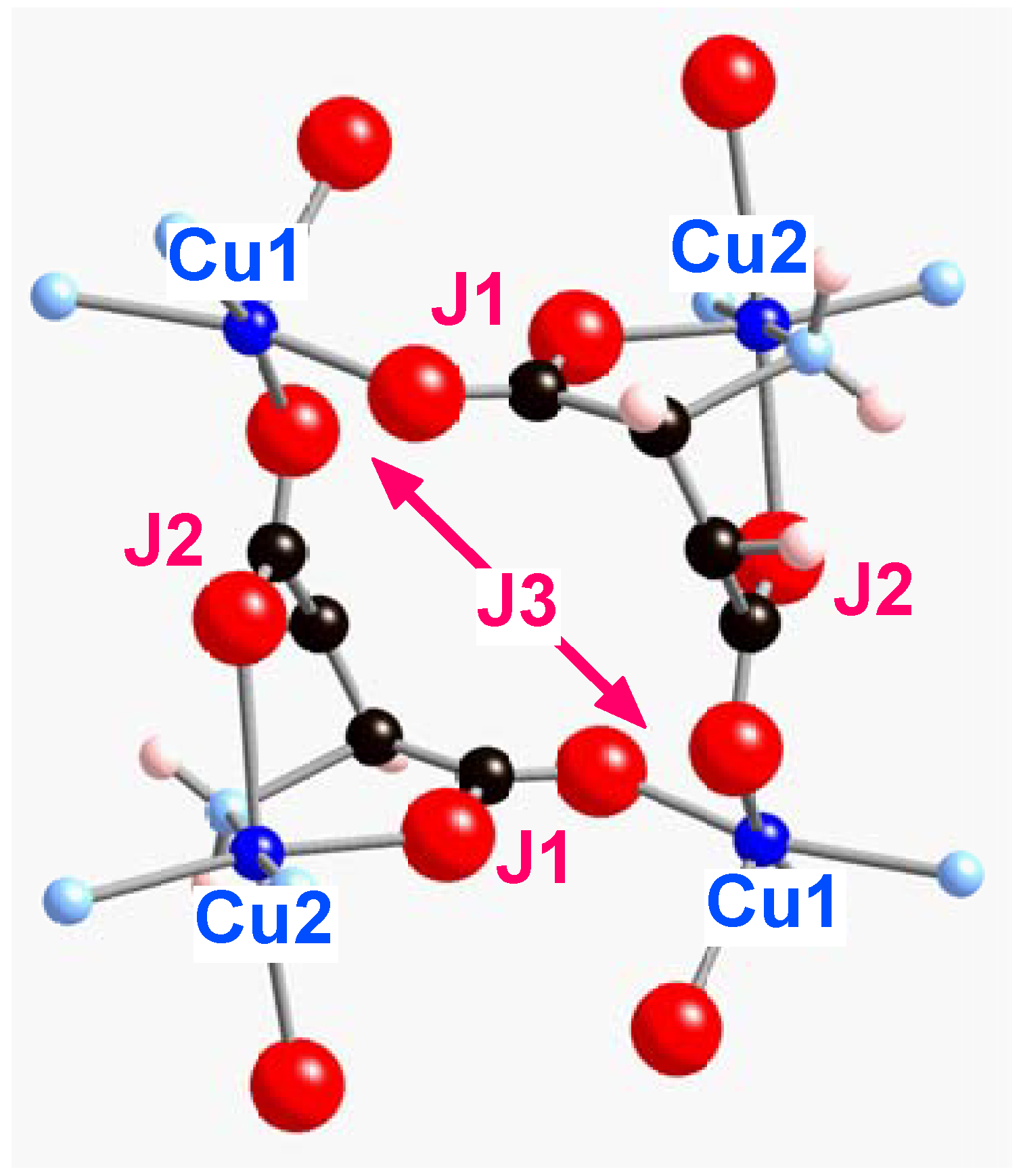
Within each of the [Cu
4(bpy)
4(aspartate)
2(H
2O)
3]
4+ clusters one can identify three through-bond Cu
II-ligand-Cu
II and a single through-space Cu
II…Cu
II magnetic pair interactions. According to
Figure 5, the different Cu
II-ligand-Cu
II pairs are Cu1-aspartate-Cu2 (equatorial-equatorial), Cu1-aspartate-Cu2 (equatorial-apical) and Cu2-aspartate-Cu2, and the through-space magnetic interaction is Cu1
…Cu1. We have identified these pairs as d
1, d
2, d
3, and d
4 respectively. The Cu
…Cu distance for dimers within each tetranuclear Cu
II cluster (
Figure 2a-
Figure 2b) is given in
Table 1. Nearby Cu
II clusters within and between
bc-planes are separated by two bpy ligands and present a Cu
…Cu distance no shorter than 8.209 and 7.363Å, respectively. The magnetic interaction for such inter-cluster Cu
…Cu dimers (d
5 and d
6 in
Table 1) is through-space and thus it is expected to be smaller than through-bond d
1-d
3 pair interactions. However, to test this fact, we also computed their value.
Table 1.
Cu…Cu distances for spin-containing metal centre pairs d1-d6 for tetranuclear [Cu4(bpy)4(aspartate)2(H2O)3]4+ clusters. Pairs d1-d3 and d4 are through-bond and through-space intra-(tetranuclear CuII cluster) magnetic interactions, respectively. Pairs d5-d6 are through-space inter-(tetranuclear CuII cluster) magnetic interactions. UB3LYP / Ahlrichs values for JAB(di) = E(BS-OSS) - E(T) in cm-1 are also given.
| tetranuclear CuII cluster1 | | dist(Cu…Cu) /Å | JAB /cm-1 | | dist(Cu…Cu) /Å | JAB /cm-1 |
|---|
| intra-cluster | (a) | | | (b) | | |
| d1 | | 5.173 | 10.6 | | 5.168 | 11.4 |
| d2 | | 5.200 | -1.8 | | 5.179 | -3.8 |
| d3 | | 7.407 | -6.7 | | 7.331 | -1.5 |
| d4 | | 7.262 | -0.06 | | 7.302 | 0.12 |
| inter-cluster | | | | | | |
| d5 | | 7.363 | <|0.02| | | | |
| d6 | | 7.521 | <|0.02| | | | |
Figure 5.
Three-dimensional view of the magnetic structure for each Cu
II tetramer (see
Figure 2a-b for specific geometries), indicating the non-negligible microscopic
JAB pair interaction parameters (bpy rings are omitted for clarity).
Figure 5.
Three-dimensional view of the magnetic structure for each Cu
II tetramer (see
Figure 2a-b for specific geometries), indicating the non-negligible microscopic
JAB pair interaction parameters (bpy rings are omitted for clarity).
We have computed the value of the microscopic
JAB parameters for all pairs above mentioned: within and between tetranuclear Cu
II clusters, i.e. d
1-d
4 and d
5-d
6, respectively, as listed in
Table 1. The two sets of
JAB values within each Cu
II cluster are similar, although there are small but non-negligible changes in the J2 (-3.8 vs. -1.8 cm
-1) and J3 (-1.5 vs. -6.7 cm
-1) parameters. The difference mainly results from small changes in the relative positions of the aspartate group in each tetranuclear cluster. We have also computed the through-space Cu1
…Cu1 interaction within each tetranuclear Cu
II cluster. The results we obtained (0.12 and -0.06 cm
-1) are small but they were also included in our simulations. As a final test we studied the inter-(Cu
II cluster) interactions, which we found to be smaller than |0.02| cm
-1. Consequently, those interactions were discarded (we have tested that their inclusion makes no change on the computed magnetic susceptibility curves). Therefore, as the two inequivalent tetranuclear Cu
II clusters (
Figure 2a-2b) are simultaneously present in the magnetic structure of the [Cu
4(bpy)
4(aspartate)
2(H
2O)
3](ClO
4)
4·2.5H
2O crystal, the minimal magnetic model that describes its magnetism is a two isolated square model, that is, a (4+4)-spin centre model, where each square has the topology depicted in
Figure 4 and
Figure 5 (with
JAB values given in
Table 1).
As the two Cu
II clusters in such minimal (4+4) model are not magnetically coupled, we have analyzed each 4-spin centre model separately. Taking each isolated square 4-spin centre magnetic model, we computed the matrix representation of the Heisenberg Hamiltonian (
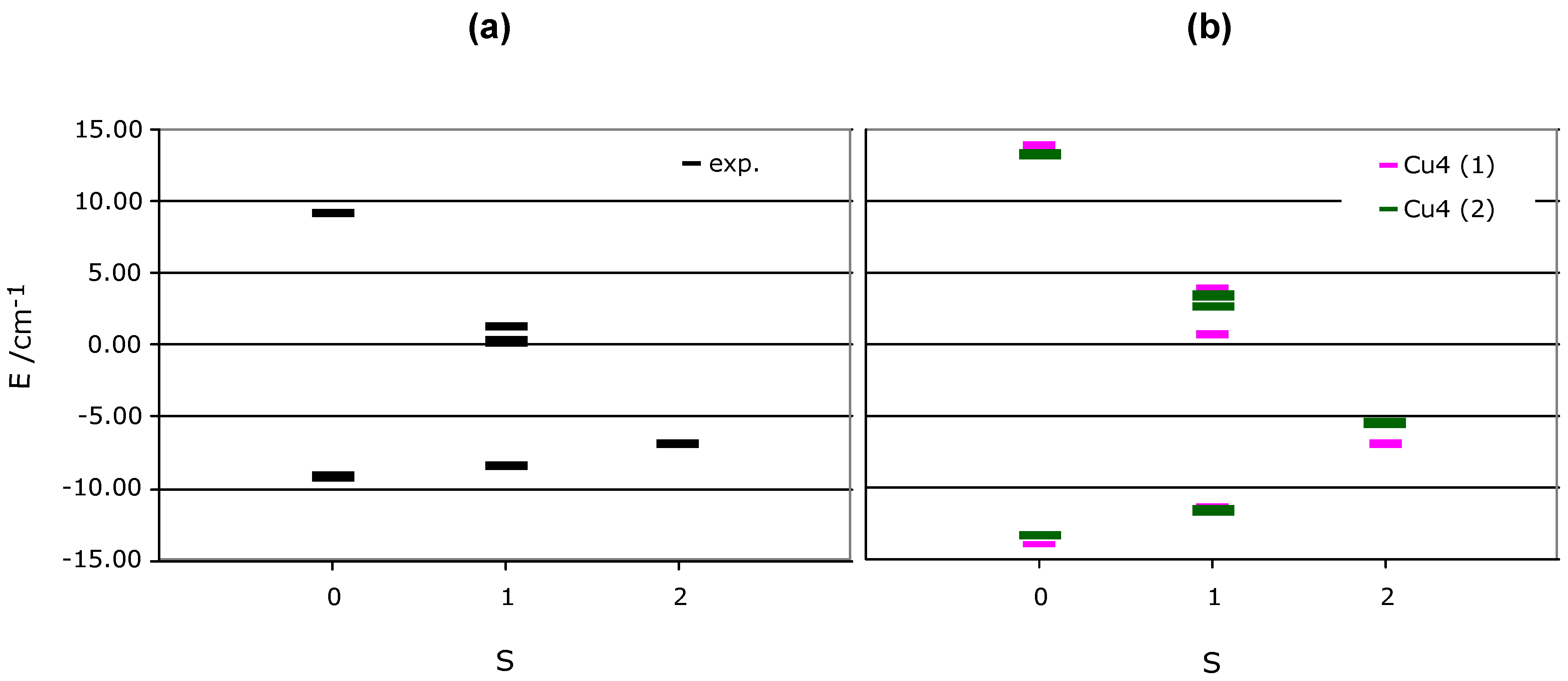
JAB in equation 1 are replaced by the computed J1, J2, J3 and J4 values) and diagonalised that matrix. We thus obtained six states (2 singlet, 3 triplet, and 1 quintet states). The energy spectra, plotted in
Figure 6b, show that the lowest energy state is a singlet, just slightly below the quintet state (1.83 and 2.47 cm
-1 in each of the Cu
II clusters). Therefore, although the ground state is antiferromagnetic and the only populated state at 0 K, the lowest triplet state can be easily populated by small variations of temperature. A further increase populates the quintet state. The triplet and quintet states are associated to the presence of ferromagnetic interactions in the tetranuclear Cu
II cluster.
Figure 6.
Representation of the relative energy of the six possible states in which one can place the four electrons present in the Cu
II tetramers of
Figure 2a-b. We have plotted in (a) the states computed when using the experimental J
ij fitted parameters (in black), and in (b) those obtained using the J
AB computed parameters for each tetramer (in purple for tetramer 2a and green for 2b).
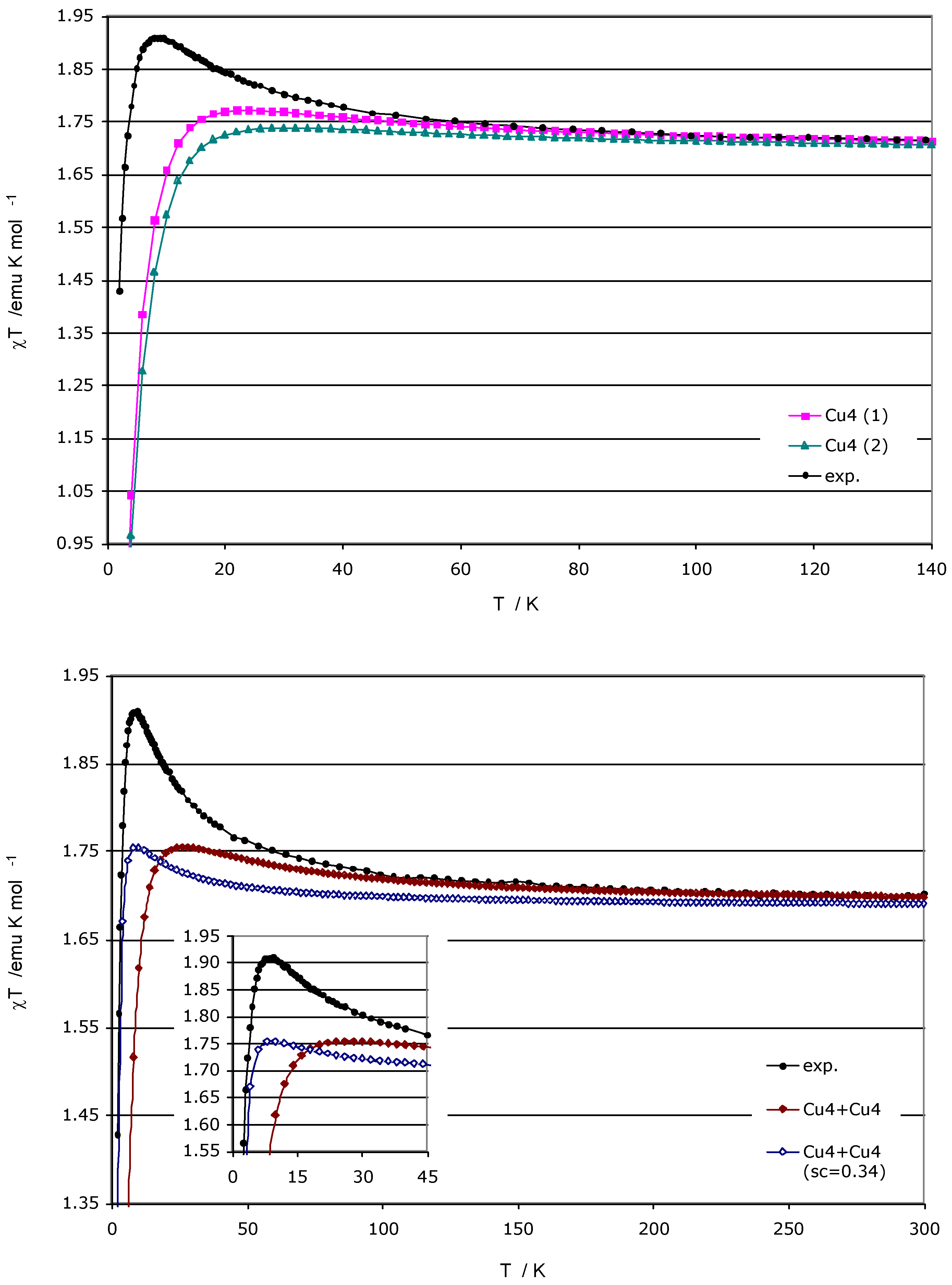
From the energy spectrum, we may then compute the magnetic susceptibility at any given temperature, and thus follow the variation of this property with temperature, as shown in
Figure 7. As the experimental data was fitted using a simple square model with 3
Jij parameters, we have first compared the experimental χT(T) curve and those obtained by using as model only one tetranuclear Cu
II cluster (a 4-spin centre model), with the two sets of
JAB constants listed in
Table 1 (
Figure 7a). No noticeable difference is appreciated comparing the χT(T) data for each cluster. We then computed the χT(T) curve using the minimal two-square model, without and with linear scaling factor in the spectrum of energy (
Figure 7b) (the linear scaling factor is of the type J
ab’ = a J
ab over all J
ab parameters, and can be visualized as a correction on the energy of all the spin states, which accounts for errors introduced by the use of DFT methods to compute the energy, instead of more sophisticated
ab initio methods, as well as for possible cooperativity and numerical errors). The shape of these χT(T) curves, with a peak around 20K, is that expected for a solid having an antiferromagnetic, S=0, ground state but having ferromagnetic interactions that are easily populated when increasing the temperature. However, none of these computed curves fully match the experimental data, not even when applying a linear scaling factor to the energy to improve the agreement. Notably the use of similar scaling factors was previously found to induce full reproducibility of the experimental magnetic susceptibility curve in purely organic molecular magnets [
4,
5].
Figure 7.
Variation of the magnetic susceptibility with the temperature. (a) Experimental curve (black) and computed curves for each of the two non-equivalent Cu
II tetramers (purple and green, according to
Figure 2a and
Figure 2b respectively); (b) Experimental curve (black) and computed curves for the two-tetramer model (8 electrons in 8 sites), without and with scaling factor (the linear scaling factor used is 0.34).
At this point we looked for possible reasons for the discrepancy between the experimental and computed magnetic susceptibility χT(T) curves. First of all, one has to note that the difference in the shape arises from changes in the relative position of the six magnetic states in the energy spectrum, and that these changes are just a consequence of variations in the
JAB values. A comparison of the fitted
Jij parameters and the computed
JAB pair interactions for each inequivalent tetranuclear Cu
II cluster indicates that the values always differ by less than 3 cm
-1. The effect that such
Jij vs.
JAB differences induce in the energy spectrum is shown in
Figure 6a-b. It shows that the relative ordering of states is always the same. However, the difference between the singlet and triplet state using either
Jij or
JAB values is three times larger in the second case (0.80 vs. 2.47 cm
-1, respectively). We have analyzed the causes for such a behaviour and found that they can be associated to the following sources: (a) need for better quality experimental magnetic susceptibility data in the low temperature region (obtained by the use of better samples, lower temperature rates, use of smaller/larger magnetic fields in the experiment, etc., (b) the use of high-temperature crystal structures instead of low-temperature structures (we have recently proven it is necessary to use low-temperature crystal data to fully reproduce the magnetic properties in purely-organic molecular magnets [
12]), (c) error accumulation in the theoretically obtained data. Work is currently under progress to investigate all these possibilities with the aim of improving the agreement between the computed and experimental χT(T) curves.


