Information Geometrical Characterization of Quantum Statistical Models in Quantum Estimation Theory


Graduate School of Informatics and Engineering, The University of Electro-Communications, 1-5-1 Chofugaoka, Chofu-shi, Tokyo 182-8585, Japan
Entropy 2019, 21(7), 703; https://doi.org/10.3390/e21070703
Submission received: 10 June 2019
/
Revised: 5 July 2019
/
Accepted: 16 July 2019
/
Published: 18 July 2019
(This article belongs to the Section Quantum Information)
Abstract
:In this paper, we classify quantum statistical models based on their information geometric properties and the estimation error bound, known as the Holevo bound, into four different classes: classical, quasi-classical, D-invariant, and asymptotically classical models. We then characterize each model by several equivalent conditions and discuss their properties. This result enables us to explore the relationships among these four models as well as reveals the geometrical understanding of quantum statistical models. In particular, we show that each class of model can be identified by comparing quantum Fisher metrics and the properties of the tangent spaces of the quantum statistical model.
1. Introduction
Information geometry about a statistical model offers simple and powerful understanding of statistical inference problems (see, for example, books [1,2,3] and the recent review on the subject [4]). A family of probability distributions is regarded as an element of a statistical manifold. Thereby, we can introduce geometrical quantities such as a Riemannian metric and affine connection. The celebrated Chentsov’s theorem selects the unique metric (up to a constant factor), called the Fisher metric or Fisher information matrix, which is invariant under the Markov map. Statistically meaningful connections are also given as a one-parameter family, known as the -connection, which exhibits the famous duality relationship.
The non-commutative extension of classical statistics to a quantum system was initiated in the 1960s by Helstrom [5] and has been one of the fundamental problems in quantum information theory until today. In particular, recent advances in quantum metrology, quantum sensing, and quantum imaging, i.e., high precision measurement methods utilizing quantum resources, has triggered many activities in the field (see reviews on these subjects [6,7,8,9,10,11]). Despite these efforts in past, there exist many open problems regarding multi-parameter estimation problems.
The information geometrical study on quantum statistical manifolds is of fundamental interest, yet is still at the developing stage [2,4,12,13]. For example, the uniqueness of Fisher metric does no longer holds in the quantum case. Instead, we have a family of operator monotone metrics on quantum statistical manifold [14]. Related to this non-uniqueness of a metric, the asymptotically achievable bound for the mean square error matrix is not expressed as a simple form of a certain quantum version of Fisher metric in general. Recent studies on the first-order asymptotic theory proves that the Holevo bound [15] can be achieved under certain regularity condition [16,17,18,19,20,21]. The Holevo bound, as defined in Section 3.1, is expressed as a nonlinear optimization problem. Hence, it is not totally clear whether we can draw any geometrical structure for it or not. Holevo introduced a particular class of quantum statistical models, called a D-invariant model, based on the invariant property of the tangent space, and showed that the right logarithmic derivative (RLD) Cramér–Rao (CR) bound can be achieved for the D-invariant model. To our knowledge, less is known regarding a connection between information geometrical properties of quantum statistical models and the Holevo bound.
One of the main motivations of this paper is to make an attempt at classifying quantum statistical models based on the Holevo bound, and then to associate these classified models with geometrical quantities. The current paper is based on the results presented in Ref. [22], where we analyzed the structure of the Holevo bound in detail for a qubit system. We derived an explicit formula for any qubit model together with characterization of special classes of the qubit models. We also classified the D-invariant model for the general qubit model together with nontrivial characterization of this model. However, we did not develop a systematic analysis of characterizations for these models in the previous study. What was missing in the previous studies was to consider two different tangent spaces in a unified manner. In this paper, we continue to explore possible classification of arbitrary quantum statistical models into several classes in which the Holevo bound can be expressed in closed formulas. By treating two tangent spaces with equal footings, we derive simple yet geometrically transparent characterizations of statistically meaningful models. Another contribution of this paper is to show that the super-operator, which was originally introduced to study the D-invariant model, also enables us to characterize other classes of quantum statistical models.
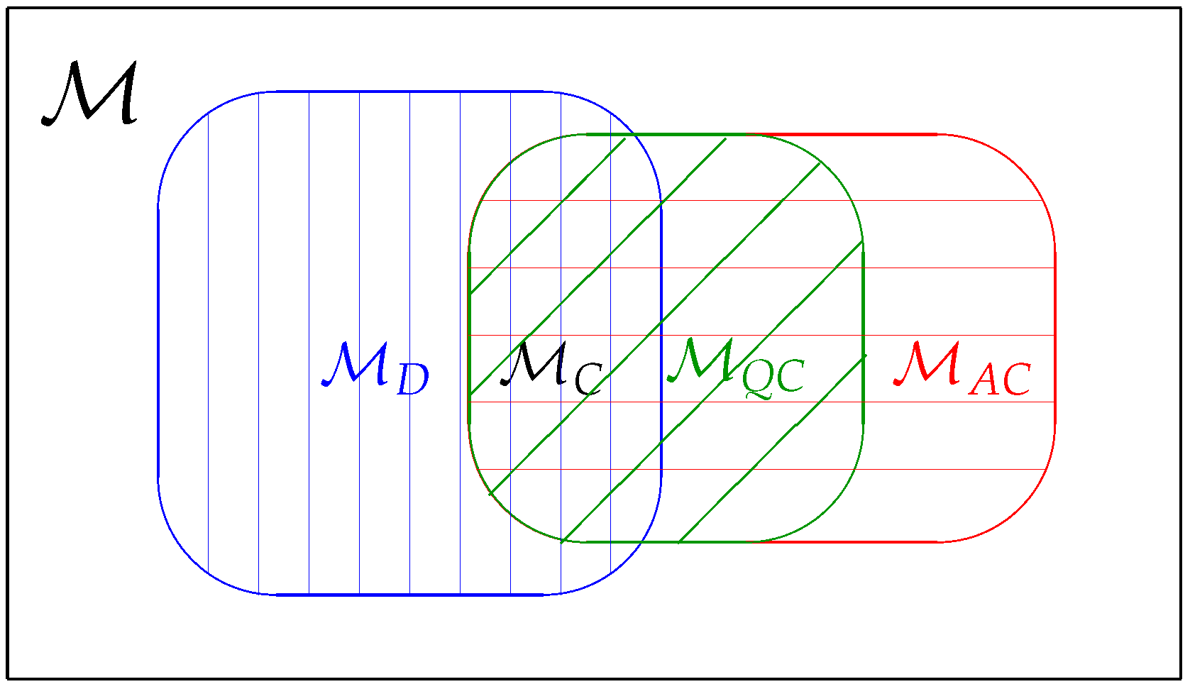
In this paper, we consider four different classes: The first class is the classical model where a quantum statistical model is reduced to a statistical model in classical statistics. The second class is known as the quasi-classical model defined by the condition imposing all quantum score operators commute with each other. The third class is known as the D-invariant model introduced by Holevo [15]. It was shown in Ref. [22] that the Holevo bound is equivalent to the RLD CR bound if and only if the model is D-invariant. The fourth class is when the Holevo bound coincides with the symmetric logarithmic derivative (SLD) CR bound. We call this class of models as the asymptotically classical in the sense that the model is asymptotically equivalent to a classical Gaussian model in the local asymptotic normality (LAN) theory [16,17,18,19,20,21]. The results of this paper are given by the propositions and theorem in Section 4.1. In Figure 1, we summarize the relations among four different classes of quantum statistical models. Figure 2 in Section 4.1 represents a schematic diagram for the main theorem of this paper. Out result shows that three classes of models can be characterized simply by comparing quantum Fisher metrics.
The content of this paper is summarized as follows. Section 2 provides preliminaries for notations and mathematical tools used in this paper. In Section 2.3, a few lemmas are proven to be useful for classifying quantum statistical models. In Section 3, we list the definitions of four different classes of statistical models. Our main results are given in the next section. Section 4.1 gives the main results of this paper. In Section 4.2, we discuss the geometrical meaning of the results in detail. Proofs for the theorem and propositions are given in Section 4.3. Several examples are discussed in Section 5 to illustrate our findings. The last section, Section 6, concludes the paper with a few remarks and open problems.
2. Preliminaries
A quantum system is a d-dimensional Hilbert space on the complex number. Denote by a set of (bounded) linear operators from to itself, and by a set of linear and hermite operators from to itself. A quantum state is a positive semi-definite operator on with unit trace. Let us denote a set of all quantum states on by and all full-ranked quantum states by . A quantum statistical model is defined by a parametric family of quantum states
where is an open subset of . As in classical statistics, we impose several regularity conditions, such as one-to-one smooth mapping, , differentiability, linearly independence of partial derivatives with respect to the coordinates , non-degeneracy for the eigenvalues, and so on. In the following discussions, we assume all these regularity conditions to avoid non-regular behaviors of the statistical model. In particular, we mainly consider a quantum statistical model of full-rank states unless stated explicitly.
2.1. Tangent Space and Quantum Fisher Metric
We define two quantum versions of the score functions, called logarithmic derivative operators, as follows. For a given quantum state and any operators , define the symmetric logarithmic derivative (SLD) and right logarithmic derivative (RLD) inner products by
respectively, where denotes the hermite conjugate of X. When X and Y are both hermite, holds. The ith SLD and RLD operators, and , are formally defined by the solutions to the operator equations:
for , where denotes the partial derivative with respect to . It is not difficult to see that the SLD operators are hermite, whereas RLD operators are not in general.
The SLD and RLD Fisher metrics, or quantum information matrices, are defined by
respectively. It is known that the SLD Fisher metric is the smallest and the real part of RLD Fisher metric is the largest operator monotone metrics on the quantum state space [14].
The SLD tangent space is defined by the linear span of SLD operators:
and the RLD tangent space is defined by the linear span of RLD operators with complex coefficients:
Let be the inverse of the SLD Fisher information matrix and be the inverse for the RLD Fisher information matrix. It is convenient to introduce the following linear combinations of the logarithmic derivative operators
By definitions, forms a dual basis for the inner product space ; , which we call the SLD dual operator. The same statement holds for the RLD case.
Noting that the SLD and RLD operators are types of exponential representations of the tangent vector , we can show the next lemma.
Lemma 1.
For , and , the following holds.
Proof.
We note that the definitions of logarithmic derivative operators give
and repeated applications of this relation proves
for any integer power k. It is then easy to prove Equation (8). □
As an application of this lemma, we have alternative expressions for the quantum Fisher information matrices:
which follow directly from definitions of and .
2.2. Commutation Operator
For a given quantum statistical model of Equation (1), we define a super-operator from to itself, whose action on is determined by the operator equation:
The super-operator , called the commutation operator at , was introduced by Holevo [15]. By definition, we can check that the super-operator is linear. Denoting the identity operator I, the following relationship holds
which can be proven by the direct calculation.
The properties useful in our discussion are given in the next lemma.
Lemma 2.
For , the following relations hold.
Proof.
The first relationship can be proven directly as
and Equation (15) can be proven similarly. □
2.3. Basic Lemmas
In this subsection, we list several lemmas that are used in our discussion. We define two hermite matrices, in terms of SLD and RLD dual operators as follows.
By definition, they are complex matrices in general. Hermiteness can be checked directly by
where denotes the complex conjugation of . Hermiteness of the matrix can be checked similarly. We remark that and are to be used to construct the quantum Fisher metrics, since they define inner products on the tangent space. However, they are not operator monotone metrics in general.
Together with the SLD and RLD Fisher information matrices, we list four matrices for comparison:
By definition, and hold, where denotes the real part of .
First, it is straightforward to see that the operator enjoys the following property.
Lemma 3.
is orthogonal to the SLD tangent space with respect to , and is orthogonal to the RLD tangent space with respect to .
Proof.
Direct calculation shows
where Lemma 1 with is used to get the second line.
Orthogonality to the RLD tangent space with respect to the RLD inner product can be proven similarly. □
The following matrix inequalities between , , , and are fundamental.
Lemma 4.
Two matrix inequalities,
hold where the necessary and sufficient condition for the equality is the same and given by , .
Proof.
Let and define an hermite matrix,
The matrix is then positive semi-definite. Using Lemma 3, we can also express matrix elements of as
where the second equality is due to Lemma 3. The third equality follows from definition of the RLD dual operator. The fourth equality is due to Lemma 1. Therefore, we show the matrix inequality . The equality is satisfied if and only if this matrix is zero. This is equivalent to for all .
The second inequality can be proven in the same way by starting with another positive semi-definite matrix . □
Next, define and consider another hermite matrix . Following exactly the same logic as in Lemma 4, we can prove the next lemma.
Lemma 5.
Two matrix inequalities
hold where the necessary and sufficient condition for the equality is the same and given by , .
Finally, the commutation operator and logarithmic operators satisfy the following relations (we note that Equation (35) in the previous publication [22] contains a typo in the same formula, thus Lemma 6 in this paper reports the corrected version). Importantly, the right hand side of each equation is expressed as the difference between two hermite matrices defined in Equation (19).
Lemma 6.
hold for , where denotes the imaginary part of .
Proof.
Using definitions of the SLD and RLD inner product, and the commutation operator, we have
for all . We now set , and then this proves Equation (23). The choice of and the use of the expressions in Equation (11) gives Equation (24). The relation in Equation (25) can be shown similarly by and . Last, if we let , we obtain Equation (26). □
3. Model Class in Quantum Statistical Models
In this section, we first define the Holevo bound. We then consider four different classes for quantum statistical models. The first class is purely classical. The second class is a quasi-classical model. The third and fourth ones are nontrivial, the D-invariant and asymptotically classical models, respectively.
3.1. Asymptotic Bound: Holevo Bound
In this subsection, we give a brief summary of the asymptotic theory on quantum state estimation [13]. As in classical statistics, we are given N-tensor product of identically and independently distributed (i.i.d.) quantum states on . We perform a measurement on , which is described by a set of matrices under certain conditions, to infer an unknown parameter value . The estimation error of the measurement is evaluated by the standard mean-square error (MSE) matrix . In the asymptotic theory of quantum state estimation, one minimizes the weighted trace of the MSE matrix under an additional condition as follows (to distinguish trace on the state space, we use for the trace on the parameter space).
where is an arbitrary positive-definite weight matrix and a.u. indicates that infimum is taken over all possible asymptotically unbiased estimators. The first-order estimation error bound in Equation (27) is usually referred to as the CR type bound in the literature. There have been many mathematical works to obtain an alternative expression for the CR bound in terms of information quantities, such as the quantum Fisher information matrix. Unlike classical statistics, where the bound is given by the Fisher information matrix, the above bound cannot be written as a simple closed formula in general. However, it takes the following optimization form known as the Holevo bound:
In this definition, the set is defined by
Introducing the hermite matrix , we define the function by
where denotes the absolute value of a linear operator X. The following theorem establishes that the Holevo bound is equal to the CR type bound.
Theorem 1.
For a quantum statistical model satisfying the regularity conditions, holds for all weight matrices.
Proofs based on different assumptions can be found in Refs. [16,17,18,19,20,21]. The Holevo bound is regarded as unification of previously known bounds [23], such as the SLD and RLD CR bounds:
Importantly, the relation holds for all [15].
3.2. Classical Model
At each point , the quantum state can be diagonalized with a unitary as , where the diagonal matrix,
lists the eigenvalues of the state . By definition, and . In other words, can be regarded as an element of the set of all (positive) probability distributions on the set . When the unitary is independent of for all point in , it is clear that any statistical problem is reduced to the classical one. With this identification, we have the following definition.
Definition 1
(Classical statistical model). For a given quantum statistical model of Equation (1), the model is said classical if the family of quantum states can be diagonalized with a θ-independent unitary U as
for all parameter values .
3.3. Quasi-Classical Model
The second class of quantum statistical models is known in the literature. It is called a quasi-classical model, which was originally introduced in Ref. [24].
Definition 2
(Quasi-classical model). A quantum statistical model of Equation (1) is said quasi-classical, if all SLD operators commute with each other at all points θ. That is,
hold for all parameter values .
Clearly, if the model is classical, then it is also quasi-classical. However, the converse statement does not hold in general. A simple counter example is discussed in Section 5.2. It is also easy to see that any one-parameter model is automatically quasi-classical.
An important property of quasi-classical models is that we can diagonalize all SLD operators simultaneously. It is then possible to perform a measurement that saturates the SLD CR bound defined in Equation (29) explicitly. Last, the concept of quasi-classical model makes sense for a particular point , if all SLDs at commute with each other.
3.4. D-Invariant Model
Holevo introduced an important class of quantum statistical models based on the commutation operator [15].
Definition 3
(D-invariant model (Holevo)). A quantum statistical model of Equation (1) is called D-invariant at θ, if the SLD tangent space at θ is an invariant subspace of the commutation operator.
Mathematically, this condition is expressed as , at . For our discussion, we focus on the D-invariant model at all (global D-invariance). For (globally) D-invariant models, the Holevo bound can be expressed analytically and coincides with the RLD CR bound [15], i.e., , , and its achievability is discussed in the literature.
3.5. Asymptotically Classical Model
The last class of quantum statistical models is when the Holevo bound coincides with the SLD CR bound.
Definition 4.
A quantum statistical model of Equation (1) is called asymptotically classical, if the Holevo bound is identical to the SLD CR bound for all positive weight matrices.
Mathematically, this definition is expressed by the condition: , .
4. Model Classification and Characterization
In this section, we give classification of quantum statistical models based on the definitions introduced in Section 3. In the following, we denote the set of all classical models, quasi-classical models, D-invariant models, and asymptotically classical models on by , , , and , respectively. We first list the results on several equivalent characterization of each model class. Discussions on the results are presented followed by the proofs in Section 4.3.
4.1. Results
4.1.1. Classical Model
The following proposition characterizes the classical model.
Proposition 1.
For a given (regular) quantum statistical model of Equation (1), the following conditions are all equivalent.
- 1.
- The model is classical (Definition 2).
- 2.
- , .
- 3.
- , .
- 4.
- .
- 5.
- , .
- 6.
- .
- 7.
- .
- 8.
- The model is D-invariant and asymptotically classical.
Here, we remind that all statements are made for the global aspect of the model, i.e., for all points .
We note that this result, equivalence between Condition 1 and Condition 4, was also stated in Ref. [25].
4.1.2. D-Invariant Model
In Ref. [22], we derived several equivalent characterizations of the D-invariant model. For readers’ convenience, we summarize them in the following proposition together with the new characterization g.
Proposition 2.
Given a quantum statistical model, the following conditions are equivalent.
- 1.
- is D-invariant at θ (Definition 3).
- 2.
- , .
- 3.
- , .
- 4.
- 5.
- , .
- 6.
- , with respect to ⇒ with respect to .
- 7.
- is an invariant subspace of the commutation operator .
4.1.3. Asymptotically Classical Model
With this notion of the asymptotically classical model, we have the following result.
Proposition 3.
For a regular quantum statistical model, the following equivalences hold:
- 1.
- is asymptotically classical (Definition 4).
- 2.
- , .
- 3.
- .
- 4.
- .
- 5.
- , .
We note that the equivalence among Conditions 1, 3, 4 and 5 were first stated in Ref. [26] without proof. Equivalence between the first and the last conditions (Conditions 1 and 5) was independently proven in Ref. [27], in which the authors named the “compatibility condition”. Condition 2 was suggested by Nagaoka (Private communication (2015)).
4.1.4. Matrices
Combining the previous lemmas and theorems with additional analysis, we can obtain another characterizations of quantum statistical models based on the four hermite matrices, . This is summarized in the next theorem.
Theorem 2.
Given a quantum statistical model, we have the following equivalences.
- 1.
- is classical. ⇔ ⇔ ⇔
- 2.
- is D-invariant. ⇔ ⇔
- 3.
- is asymptotically classical. ⇔
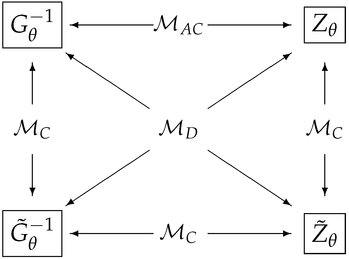
Figure 2 gives a schematic diagram summarizing the relations among the matrices and corresponding model classification. We can classify three models simply by comparing these four matrices. Proof of this theorem is given in Section 4.3.4.
As the corollary, we can characterize models by the properties of two tangent spaces and .
Corollary 1.
Given a quantum statistical model, we have the following equivalences.
Proof of this corollary is immediate from Theorem 2 and use of Lemmas 1, 2, and 6.
4.2. Discussion on the Results
In this subsection, we discuss the geometrical meaning and statistical consequences of the results: Propositions 1, 2, 3, Theorem 2, and Corollary 1.
4.2.1. Tangent Vector
We first note that Conditions 2 and 3 in Proposition 1 are nothing but the condition in Equation (35) in Section 4.3. This is straightforward to understand if we regard as an m-representation of the tangent vector and as an e-representation of it with respect to the SLD Fisher metric. The statement applies for the RLD case.
Next, we can compare Condition 5 in Proposition 1 to the condition for the D-invariant model, Condition 5 of Proposition 2: for all i. For the quasi-classical model, we have conditions of for all by definition. The asymptotically classical model, on the other hand, only requires commutativity of the SLD operators on the support as indicated by Condition 5 in Proposition 3.
4.2.2. Quantum Fisher Metric
Condition 4 in Proposition 1 states that the SLD and RLD quantum Fisher metrics are identical. If this is the case, in fact, all possible monotone metric on are identical. In other words, they collapse to the single monotone metric. This is because: (1) the imaginary part of the RLD Fisher metric vanishes; and (2) the SLD Fisher metric is the minimum and the real RLD Fisher metric is the maximum monotone metric (Petz’s theorem) [14]. Due to Theorem 2, this condition is also equivalent to and .
Next, let us consider the D-invariant model. Condition 4 of Proposition 2 requires that the real part of the inverse of the RLD Fisher metric is identical to that of the SLD Fisher metric. In addition, the imaginary part of the inverse of the RLD Fisher metric needs to be the same as that of matrix. By Theorem 2, its dualistic condition is shown to be equivalent.
Last, the asymptotically classical model only requires that the imaginary part of the matrix (Condition 3 of Proposition 3). From this fact, we can easily understand the reason the classical model is equivalent to the D-invariant and asymptotically classical model.
4.2.3. Tangent Space
As the fundamental objects in information geometry, let us analyze the SLD tangent space . Condition 6 in Proposition 1 means that the SLD tangent space is in the kernel of the commutation operator , whereas the SLD tangent space is an invariant subspace of the commutation operator for the D-invariant model. Next, the asymptotically classical model is characterized by the condition that and are mutually orthogonal subspaces. In other words, the action of the commutation operator takes all elements of the SLD tangent space to the outside of this space.
We split the SLD operator into two parts, namely a classical part and a quantum part, where the latter is defined by the change in a unitary direction. Since the operator maps the commutation relationship to the anti-commutation relationship as in Equation (12), the quantum part of the SLD operator is expressed in terms of the commutation operator. With more analysis, we can show that the condition for the classical model is equivalent to vanishing of the quantum part of SLD operators (see also the discussion given in Ch. 7 of the book [2]).
4.2.4. Asymptotic Bound
The last equivalent condition, Condition 8 in Proposition 1, is a rather straightforward consequence once we combine all ingredients presented in the lemmas and other equivalent conditions for the classical model. However, the statistical implication of this condition is nontrivial in the sense that we only consider properties of asymptotically achievable bounds. One is the bound for the D-invariant model, and the other is the bound for the asymptotically classical model. Another implication of this equivalence is that there is no genuine quantum statistical model that is both D-invariant and asymptotically classical. In this sense, these two classes of quantum statistical models, the D-invariant and asymptotically classical models, are regarded as two extremal and mutually exclusive models.
4.3. Proofs
As stated bove, all conditions in this section are about all parameter values unless otherwise stated.
4.3.1. Proof for Proposition 1
Proof.
Equivalence to Conditions 2 and 3:
First, we note that the definition of the classical model is equivalent to the commutativity of for all different values , that is,
By the standard matrix analysis, this is equivalent to:
From the definitions of the SLD and RLD operators, we can show that the condition in Equation (35) is equivalent to for all i. This is Condition 2. Similarly, Condition (35) can be converted to for all i, which is Condition 3.
Equivalence to Conditions 4 and 5:
If the model is classical, the SLD operator commutes with the quantum state. Hence, operator formulas in Equation (3) defining the SLD and RLD operators are identical. Since the SLD and RLD operator are uniquely defined, we obtain for all i.
Next, assuming Condition 5, matrices and are identical. Noting , we get Condition 4.
Last, suppose Condition 4, , then, from Lemma 3, this is possible if and only if and for all i. Since , the latter condition leads to for all .
Equivalence to Conditions 6 and 7:
Condition 6 is to say that the SLD tangent space is in the kernel of the commutation operator. From definition of the commutation operator and the fact that implies if , we have
This then immediately establishes equivalence between Conditions 2 and 6. A similar argument applies for Condition 7.
Equivalence to Condition 8:
When the model is classical, Conditions 4 and 5 give for all i (D-invariance). Combining it with leads to . Hence, the definitions for D-invariant and asymptotically classical model are clearly satisfied, if the model is classical. Conversely, suppose that the model is D-invariant, , and asymptotically classical, . Then, it gives Condition 4, .
4.3.2. Proof for Proposition 2
Proof.
We only need to prove Condition 7 is equivalent to other conditions. When a model is D-invariant, and hold. Hence, it is straightforward to see is an invariant subspace. Next, suppose , i.e., . This then yields by taking the inner product with with respect to the RLD inner product and the use of . This relation is reduced to , which is equivalent to . □
4.3.3. Proof for Proposition 3
Proof.
First: The third condition implies . This is because of and the direct substitution gives
Here, is the collection of SLD dual operators. This means the set of SLD dual operators is the optimal achieving the lowest value in the definition of the Holevo bound in Equation (28).
By definition, the first condition obviously implies the second one: , .
To show that the existence of a weight matrix satisfying implies the vanishing of the imaginary part of the matrix , we prove the contraposition. That is, if , then holds for all weight matrices W. Let us use the following substitution for optimizing the Holevo function:
where () are tangent operators orthogonal to all SLD operators with respect to the SLD inner product. With this, the Holevo function reads
where matrix is hermite. We note that the last two terms:
is strictly positive since it vanishes if and only if and hold. However, these two conditions cannot be satisfied due to the assumption and the positivity of the matrix . Therefore, we show that if , we have for all . Finally, can be shown by elementary algebra. Collecting these arguments proves Proposition 3. □
4.3.4. Proof for Theorem 2
Proof.
Equivalence in Condition 1:
Since , the first equivalence is immediate.
To prove the second equivalence to in Condition 1, let us assume first that a model is classical. Condition 7 of Proposition 1 gives
Then, Equation (26) of Lemma 6 yields for all . Conversely, if holds, we have the following equivalence from the first matrix inequality in Lemma 5.
This proves the converse part.
The last equivalence to in Condition 1 is proven as follows. A classical model gives this condition is straightforward. Conversely, if this condition is satisfied, the second matrix inequality of Lemma 4 is then expressed as
Noting , this inequality concludes . (Otherwise, the matrix inequality does not hold.) This then shows that the model is asymptotically classical, and we have . The condition holds if and only if the model is D-invariant from Lemma 4. Therefore, the model is asymptotically classical and D-invariant, i.e., the classical model.
Equivalence in Condition 2:
The first equivalence is already proven in Proposition 3, whose proof is given in Ref. [22]. Here, we note that both conditions can be proven immediately if we use Lemma 4.
Equivalence in Condition 3:
This is proven in Proposition 3. □
5. Examples
5.1. Qubit Models
When the dimension of the Hilbert space is two, i.e., a qubit system, we can explicitly work out classification of models [22]. To analyze a given qubit model, it is convenient to use the Bloch vector representation of qubit states (see, for example, [15]). Define a three-dimensional real vector for by
where are the standard Pauli matrices. Since the mapping is bijective, a quantum statistical model for the qubit case can be defined as
The positivity condition is equivalent to . Based on the Bloch vector , we can derive closed formulas for the quantum score functions (SLD and RLD logarithmic derivative operators) and the quantum Fisher information matrices (see, for example, [22]) In Ref. [22], we derived the following conditions for a model of Equation (41) to be the D-invariant and asymptotically classical.
- is D-invariant. ⇔ is independent of .
- is asymptotically classical. ⇔ () is orthogonal to .
The equivalent condition for the D-invariant model immediately tells us that any unitary model on the qubit system is D-invariant. The converse statement is, of course, not true in general. For example, the following two-parameter qubit model is D-invariant, but not unitary.
where is a fixed constant and the parameters takes values within the region satisfying the positivity condition for the state.
Next, we can work out whether or not there exists a classical qubit model. It is straightforward to show that there cannot be any multi-parameter classical qubit model under the regularity condition, and thus only one-parameter classical model exists. The reason is simply because there can be a single parameter classical model embedded in a matrix space. Any multi-parameter classical model becomes a non-regular model.
Finally, we ask if there exists a quasi-classical model in a qubit system. It turns out that there exists no such a quasi-classical qubit model. This is because imposing commutativity between the SLD operators leads to a non-regular model.
To prove this statement, we note the commutation condition for the SLD operators is expressed in terms of the Bloch vectors as
Consider a two-parameter qubit model. The condition is equivalent to linearly dependence of two vectors , . This then implies the existence of a function such that holds. This contradicts with linearly independence of the tangent vectors. Note that, if this is the case, the dimension of the tangent space is one rather than two. The case of three-parameter models can be checked similarly.
5.2. Non-Classical Quasi-Classical Model
As mentioned in Section 3.3, there exists a quantum statistical model that is quasi-classical (all SLD operators commute with each other) and yet non-classical. It is straightforward to observe that such cases arise if a model is non-regular. For example, quantum states are not full rank. Below, we give a simple regular statistical model in a three-dimensional quantum system ().
We consider the following two-parameter model:
where
with the constant () and smooth function being chosen arbitrary as long as the corresponding classical model for
satisfies . The SLD operators are calculated as
where , . To have a regular quantum model, we also impose for all . It is clear that two SLD operators commute with each other for all . The RLD operators are
We can show that the SLD Fisher information matrix is diagonal and is given by
whereas the RLD Fisher information matrix is
It is easy to see that with equality if and only if , which is excluded. Therefore, holds and this model is not classical by Proposition 1.
6. Concluding Remarks
We derive several equivalent characterizations of quantum statistical models based on the estimation error bound, the Holevo bound, and information geometric properties. This then yields a simple classification of quantum statistical models by calculating information matrices. Our results immediately provide practical advantages for classifying important classes of quantum statistical models in quantum metrology [6,7,8,9,10,11]. Three classes are mainly discussed in this paper: the classical model, D-invariant model, and asymptotically classical model. We also give relationships among these classes. In particular, the classical model can be viewed as the intersection of the D-invariant and asymptotically classical models. These three models have different interpretations based on the information geometrical point of view.
Before closing the paper, we list two open questions to be addressed. In this paper, we focus on the global aspects of the quantum statistical models only. The first extension is then to analyze local properties of each class of the quantum statistical model. In Ref. [22], we analyzed the local properties for the D-invariant and asymptotically classical models. Therefore, it is interesting to see whether the local classical model is a useful concept or not. Second, we only use two quantum Fisher metrics, the SLD and RLD Fisher metrics, together with their variants and . We expect that other families of quantum Fisher metrics should also give model classification and characterization.
Funding
The work was partly supported by JSPS KAKENHI Grant Number JP17K05571.
Acknowledgments
The author would like to thank S. Ragy for providing information about their results prior to publication [27].
Conflicts of Interest
The author declares no conflict of interest.
References
- Amari, S.-I. Differential-Geometrical Methods in Statistics; Springer: Berlin/Heidelberg, Germany, 1985; Volume 28. [Google Scholar]
- Amari, S.; Nagaoka, H. Methods of Information Geometry (Translations of Mathematical Monographs); American Mathematical Society: Providence, RI, USA, 2000; Volume 191. [Google Scholar]
- Ay, N.; Jost, J.; Le, H.V.; Schwachhöfer, L. Information Geometry; Springer Nature: Gewerbestrasse, Switzerland, 2017. [Google Scholar]
- Felice, D.; Cafaro, C.; Mancini, S. Information geometric methods for complexity. CHAOS 2018, 28, 032101. [Google Scholar] [CrossRef] [PubMed]
- Helstrom, C.W. Quantum Detection and Estimation Theory; Academic Press: New York, NY, USA, 1976. [Google Scholar]
- Giovannetti, V.; Lloyd, S.; Maccone, L. Advances in quantum metrology. Nat. Photonics 2011, 5, 222–229. [Google Scholar] [CrossRef]
- Tóth, G.; Apellaniz, I. Quantum metrology from a quantum information science perspective. J. Phys. A Math. Theor. 2014, 47, 424006. [Google Scholar] [CrossRef]
- Demkowicz-Dobrzański, R.; Jarzyna, M.; Kołodyński, J. Quantum Limits in Optical Interferometry. Prog. Opt. 2015, 60, 345–435. [Google Scholar]
- Pezzé, L.; Smerzi, A. Quantum theory of phase estimation. In Atom Interferometry; Tino, G.M., Kasevich, M.A., Eds.; IOS Press: Amsterdam, The Netherlands, 2014; pp. 691–741. [Google Scholar]
- Szczykulska, M.; Baumgratz, T.; Datta, A. Multi-parameter quantum metrology. Adv. Phys. X 2016, 1, 621–639. [Google Scholar] [CrossRef]
- Degen, C.L.; Reinhard, F.; Cappellaro, P. Quantum sensing. Rev. Mod. Phys. 2017, 89, 035002. [Google Scholar] [CrossRef] [Green Version]
- Nagaoka, H. On the parameter estimation problem for quantum statistical models. In Proceedings of the 12th International Symposium on Information Theory and Its Applications (ISITA), Inuyama, Japan, 6–9 December 1989; pp. 577–582. [Google Scholar]
- Hayashi, M. (Ed.) Asymptotic Theory of Quantum Statistical Inference: Selected Papers; World Scientific: Singapore, 2005. [Google Scholar]
- Petz, D. Quantum Information Theory and Quantum Statistics; Springer: Berlin/Heidelberg, Germany, 2008. [Google Scholar]
- Holevo, A.S. Probabilistic and Statistical Aspects of Quantum Theory, 2nd ed.; Edizioni della Normale: Pisa, Italy, 2011. [Google Scholar]
- Hayashi, M.; Matsumoto, K. Asymptotic performance of optimal state estimation in qubit system. J. Math. Phys. 2008, 49, 102101. [Google Scholar] [CrossRef]
- Guţă, M.; Kahn, J. Local asymptotic normality for qubit states. Phys. Rev. A 2006, 73, 052108. [Google Scholar] [CrossRef] [Green Version]
- Kahn, J.; Guţă, J. Local asymptotic normality in quantum statistics. Commun. Math. Phys. 2009, 289, 341–379. [Google Scholar] [CrossRef]
- Yamagata, K.; Fujiwara, A.; Gill, R.D. Quantum local asymptotic normality based on a new quantum likelihood ratio. Ann. Stat. 2013, 41, 2197–2217. [Google Scholar] [CrossRef]
- Fujiwara, A.; Yamagata, K. Noncommutative Lebesgue decomposition with application to quantum local asymptotic normality. arXiv 2017, arXiv:1703.07535. [Google Scholar]
- Yang, Y.; Chiribella, G.; Hayashi, M. Attaining the ultimate precision limit in quantum state estimation. Commun. Math. Phys. 2019, 368, 223–293. [Google Scholar] [CrossRef]
- Suzuki, J. Explicit formula for the Holevo bound for two-parameter qubit-state estimation problem. J. Math. Phys. 2016, 57, 042201. [Google Scholar] [CrossRef] [Green Version]
- Nagaoka, H. A New Approach to Cramér-Rao Bounds for Quantum State Estimation; IEICE Technical Report; IEICE: Tokyo, Japan, 1989; pp. 9–14. [Google Scholar]
- Nagaoka, H. On Fisher information of quantum statistical models. In Proceedings of the 10th Symposium on Information Theory and Its Applications (SITA), Yokohama, Japan, 19–21 November 1987; pp. 241–246. [Google Scholar]
- Matsumoto, K. A Geometrical Approach to Quantum Estimation Theory. Ph.D. Thesis, University of Tokyo, Tokyo, Japan, 1997. [Google Scholar]
- Suzuki, J. Explicit formula for the Holevo bound for two-parameter qubit estimation problems. In Proceedings of the 32nd Quantum Information Technology Symposium (QIT32), Suita, Japan, 26 May 2015; pp. 125–130. [Google Scholar]
- Ragy, S.; Jarzyna, M.; Demkowicz-Dobrzański, R. Compatibility in multiparameter quantum metrology. Phys. Rev. A 2016, 94, 052108. [Google Scholar] [CrossRef] [Green Version]
Figure 1.
A schematic diagram for model classification of quantum parametric models. A generic quantum parametric model is indicated by the rectangular box. The blue vertically shadowed area represents the D-invariant model. The red horizontally shadowed area is the asymptotically classical model. The green diagonally shadowed area is the quasi-classical model. The intersection of the D-invariant model and the asymptotically classical model represents the classical model.

Figure 2.
A schematic diagram for model classification for three classes: the classical (), D-invariant (), and asymptotically classical () in terms of four matrices . Two arrows in the opposite direction indicate if two matrices are identical, and the model belongs to a class indicated between these arrows.

© 2019 by the author. Licensee MDPI, Basel, Switzerland. This article is an open access article distributed under the terms and conditions of the Creative Commons Attribution (CC BY) license (http://creativecommons.org/licenses/by/4.0/).
Share and Cite
MDPI and ACS Style
Suzuki, J. Information Geometrical Characterization of Quantum Statistical Models in Quantum Estimation Theory. Entropy 2019, 21, 703. https://doi.org/10.3390/e21070703
AMA Style
Suzuki J. Information Geometrical Characterization of Quantum Statistical Models in Quantum Estimation Theory. Entropy. 2019; 21(7):703. https://doi.org/10.3390/e21070703
Chicago/Turabian StyleSuzuki, Jun. 2019. "Information Geometrical Characterization of Quantum Statistical Models in Quantum Estimation Theory" Entropy 21, no. 7: 703. https://doi.org/10.3390/e21070703
Note that from the first issue of 2016, this journal uses article numbers instead of page numbers. See further details here.