Optimization and Entropy Production: Application to Carnot-Like Refrigeration Machines


1
Department of Engineering Thermodynamics, University POLITEHNICA of Bucharest, 060042 Bucharest, Romania
2
LEMTA, URA CNRS 7563, University of Lorraine, 54518 Vandoeuvre-lès-Nancy, France
*
Author to whom correspondence should be addressed.
Entropy 2018, 20(12), 953; https://doi.org/10.3390/e20120953
Submission received: 6 November 2018
/
Revised: 3 December 2018
/
Accepted: 8 December 2018
/
Published: 11 December 2018
(This article belongs to the Special Issue Second Law: Survey and Application)
Abstract
:Several optimization models of irreversible reverse cycle machines have been developed based on different optimization criteria in the literature, most of them using linear heat transfer laws at the source and sink. This raises the issue how close to actual operation conditions they are, since the heat transfer law on the phase-change processes is dependent on ΔT3. This paper addresses this issue by proposing a general model for study and optimization of thermal machines with two heat reservoirs applied to a Carnot-like refrigerator, with non-linear heat transfer laws and internal and external irreversibility. The optimization was performed using First and Second Law of Thermodynamics and the Lagrange multipliers method. Thus, several constraints were imposed to the system, also different objective functions were considered, allowing finding the optimum operating conditions, as well as the limited variation ranges of the system parameters. Results show that the nature of the heat transfer laws affects the optimum values of system parameters for obtaining maximum performances and also their magnitude. Sensitivity studies with respect to system several parameters are presented. The results contribute to the understanding of the system limits in operation under different constraints and allow choosing the most convenient variables in given circumstances.
1. Introduction
The second half of the last century saw the emergence of a new branch of Thermodynamics, called Thermodynamics in Finite Time, due to the process duration that was considered by the heat transfer rate [1,2]. The corresponding approach emphasized a maximum power regime [3] for an endo-reversible, but exo-irreversible engine. The engine efficiency at maximum power regime is less than the Carnot cycle one, and it introduced the particular form of the “nice radical”.
Since then, quite a lot of works analyzing the exo-irreversible engines have been developed [4,5]. Generally, they have considered only the external irreversibility of the thermal machine, which is due to the heat transfer at finite temperature difference between the sources and the working fluid. Also, mainly the linear form of the heat transfer law was used.
The same approach applied to the study of heat pumps shows no more optimum for the useful effect (heat flow delivered at the hot end), because the temperature of the working fluid has no upper limit imposed on the hot end [6]. The same happens for the refrigerating machine, where there is no lower limit to the cold end (as for thermal engine).
To the first reported work (to our knowledge) [6], other papers followed [7,8,9] dealing with heat pump or refrigerating machine optimization, but introducing an additional constraint (mostly mechanical power or useful effect imposed). The optimization is not reserved only to vapor mechanical compression machines, but it has been extended since that time to the trithermal and quadrithermal ones [10,11,12]. However, one notes that most of the reported studies deal with thermostats at sources and sinks and linear heat transfer laws.
Proposals have been made to extend the analysis by using other forms of the heat transfer law [13,14,15]. Further progress has been made by introducing an irreversibility factor (ratio), most often constant [16], that accounts for the internal irreversibility of the machine (endo-irreversibility). A step further [17] represents the internal irreversibility considered in the model as internal entropy production rate, . This method is preferred to the one of ratios, as we still see in recent work [18]. It provides a more general approach compared to the use of the irreversibility factor [16,19,20]. Also, it aims the entropic analysis of machines and processes and is more and more important as an instrument getting modeling closer to real operation [21,22,23,24,25,26,27].
The present work proposes a general model of study and optimization of irreversible Carnot-like refrigerating machines and extends the previous studies [28,29,30,31]. In terms of optimization, it is well known that several objective functions can be chosen: maximum of coefficient of performance (COP), minimum of energy consumption, minimum of total entropy production, or economic objectives [32]. Environmental concerns have also become predominant [33], and recently led to the introduction of a new objective called Ecological COP (ECOP) [34]. Two objective functions will be considered here for each of the two studied cases: maximum refrigeration load and minimum total entropy production rate when COP is imposed, respectively, maximum COP and minimum total entropy production rate, for imposed refrigeration load. We limit the presentation only to these cases as the main target is to show how the method is applied and what the relevance of the obtained results is, but it could be extended and applied for other cases of imposed constraints, such as consumed mechanical power or heat transfer restricted at the hot source, for which objective functions could be sought.
The mathematical approach includes the most general laws of science, namely the First and Second Laws of Thermodynamics. The equations of heat transfer at the hot and cold side of the machine are modeled by non-linear functions of the temperature difference between the reservoirs and the cycle working fluid. The internal irreversibility is introduced by the method of internal entropy production rate, above mentioned. Three variation laws with temperature for the internal entropy production are considered in an attempt to approach analytical treatment of actual operation.
The purpose of this work is to study the influence of the non-linearity of the heat transfer law on the performance. This will extend the model validity beyond the convective and radiative heat transfer laws [13]. The results highlight the existence of optimal operating regimes of the reverse cycle machine subjected to dimensional and operating constraints. The sensitivity study with respect to the model parameters provides interesting results related to the limitation of the variation range of the variables of the model, and different operating regime of the refrigeration machine. The new and important results reported here are presently extended by the study of other cases of imposed constraints.
2. Materials and Methods
2.1. Proposed Application Study
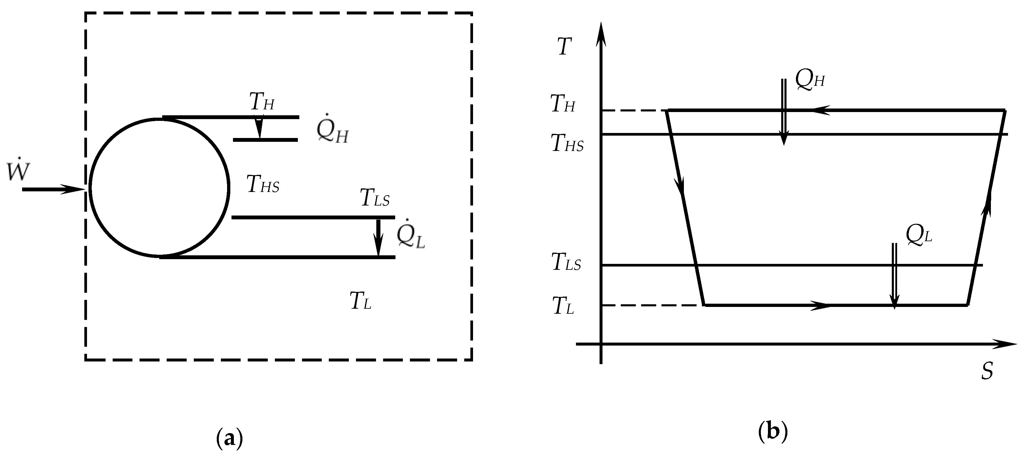
The model of study and optimization of Carnot-like machines is applied here to an irreversible refrigeration machine. Its architecture and the corresponding irreversible cycle consisting of two isothermal processes and two adiabatic irreversible ones are illustrated in Figure 1. The irreversibility is present in the T-S diagram by the entropy production on the adiabatic processes (compression and expansion), which is mainly due to internal losses. On the isothermal processes, it is marked by the different heat transfer compared to the corresponding reversible processes (also more reduced at the source and larger at the sink).
Usually, the internal irreversibility of the machine, introduced in the model as a parameter, is represented by the corresponding internal entropy production term, . It takes into account the internal irreversibility generated on each cycle process, summing the throttling losses, friction ones, etc. To this one an external irreversibility is added, being generated by finite temperature heat transfer processes between the working fluid and the heat reservoirs.
As shown in Figure 1, the two heat reservoirs are thermostats, of constant temperatures THS and TLS, the first one being actually the environment. The refrigeration machine is considered operating in steady state regime.
2.2. Mathematical Model
The model of study and optimization of reverse cycle machines is developed by using the most general laws in Thermodynamics, the First and Second Law, to which generalized forms of heat transfer laws applied to the source and sink are added.
By taking account of the sign convention adopted here, that considers the heat transfer rate positive when entering the cycle, and negative for leaving it, and the consumed work transfer rate (power request) as negative, the expression of the First Law of Thermodynamics can be written as:
with —mechanical power supplied; —heat transfer rate rejected by the working fluid at the source (hot heat exchanger); —refrigeration load.
When looking the machine irreversibility, the Second Law of Thermodynamics takes different expressions, as applied to two possible systems. Thus, once considering only the internal irreversibilities (endo-irreversible machine) by the internal entropy production term, it becomes:
with TH—temperature of the working fluid at the machine hot temperature side; TL —temperature of the working fluid at the machine low temperature side; —ntropy production due to internal irreversibilities of the machine.
Then, when the whole system is considered (cycle and the two heat reservoirs), the total entropy production term appears in the Second Law expression:
with THS—source temperature at the machine hot part; TLS—source temperature at the machine cold part; —total entropy production (internal and external).
For the heat transfer rates present in the above equations, two forms of non-linear heat transfer laws between the heat reservoirs and working fluid are considered:
where ni is the exponent of the heat transfer law (H—hot sink or high temperature side, L—cold source or low temperature side).
In practical application these non-linear forms correspond to phase-change heat transfer (Equation (4), with ni = 3), respectively radiation heat transfer (Equation (5) with ni = 4). One note that making ni = 1, one gets the linear approximation, so called, convective heat transfer law or Newton’s law.
For the refrigeration machines performance evaluation, according to its definition, the coefficient of performance is:
By combining the two expressions of the Second Law, given by Equations (2) and (3), the total entropy production rate results as:
The three positive terms contained in the above expression accounts for different type of irreversibility, namely (1) the internal one by , and (2) the external one due to finite temperature heat transfer processes between the heat reservoirs and working fluid.
Without insight in the internal irreversibility mechanism of machine processes, it is difficult to establish a variation law for the internal entropy production. Thus, in order to provide generality to the model, the following approaches were considered [35,36]:
(a) constant
(b) linear variation law with working fluid temperature difference:
(c) logarithmic variation law with working fluid temperature ratio:
2.3. Dimensionless Model
The same concern for developing a general model for the optimization of refrigeration machines and easily adapted to different characteristics and constraints of the studied case, led to the adoption of the non-dimensional form of the equations. Therefore, the following terms and expressions will be further used:
- Dimensionless temperatures are expressed relative to the reference temperature THS which is also the ambient one:
- Dimensionless energy fluxes are expressed relative to the product , where is the heat rate capacity of the working gas corresponding to the end of the compression process:
- -
- at the sink or machine cold part (positive):
- -
- at the source or machine hot part (always negative)
- -
- power supply:
- Non-linear thermal conductances are expressed relative to the product :
- -
- total one:
- -
- of the two heat exchangers:
- Internal and total entropy production terms use the same heat rate capacity, , as reference:
- The dimensionless constraint relative to a fixed total heat exchanger conductance will have as equivalent:which will be considered as optimization constraint finite parameter, while CTQH,gen and CTQL,gen are system optimization variables.
According to the adopted sign convention and the refrigeration machine scheme, the temperatures hierarchy is TL < TLS < THS < TH, that imposes the following constraints:
These constraints will always be valid for any refrigerator being studied, regardless of the presence of any other restrictions imposed by the user or the machine design.
2.4. Optimization Method and Studied Cases
The dimensionless variables that will be used in the optimization procedure are θL and CTQL,gen, θH and CTQH,gen, while the considered parameters are: θLS, CTQT,gen, , and the imposed performance characteristics.
The optimization is achieved for two cases where different performances are imposed. For a refrigeration machine, the most important performances are the COP and the refrigeration load.
The first studied case corresponds to an imposed value of the COP, together with an imposed internal entropy production rate. The objective functions could be: maximum refrigeration load, minimum total dissipation (minimum total entropy production), or minimum power consumption.
Among them, results will be reported here when the maximum refrigerating load is sought, respectively, minimum total entropy production rate.
The second optimization is done for an imposed refrigerating load, together with an imposed internal entropy production rate. Thus, other objective functions will be sought, such as maximum COP, minimum total dissipation, or minimum power consumption. Again, only the first two objective functions previously cited will be considered in this analysis, for the sake of comprehensible presentation but the method is similarly applied.
The optimization procedure uses the Lagrange Multipliers Method that will lead to a system of equations for each objective function, and its solution will provide optimal values of the control variables of the system, θL, CTQL,gen, θH, CTQH,gen, leading to the corresponding system performances achieved in the considered constraint operation. Thus, the Lagrangian function corresponding to the present study is expressed as:
where: FO is one of the considered objective functions stated above; λ1 and λ2 are the corresponding Lagrange multipliers; C1 and C2 are the problem constraints represented by the First Law of Thermodynamics including the imposed performance characteristic constraint and Second Law of Thermodynamics applied to the cycle including the internal entropy production restriction.
The optimal values of the model variables are obtained by solving the following system of equations:
2.4.1. Imposed Coefficient of Performance
The First Law of Thermodynamics combined with Equation (13) and Equations (12a)–(12b) that takes into account the expressions of generalized heat transfer laws provides:
By generalizing the above expression, the first constraint equation (C1) of the model results as:
where the following notations of the new functions were used:
One notes that f is a function of θH only, while ξ is a function of θL only. The Second Law of Thermodynamics combined with Equations (12a)–(12b) and applied to the cycle gives:
and considering the two function introduced by Equation (25), the second constraint (C2) of the system results as:
One notes that g is a function of both θH and de θL according to the three variation laws adopted for the entropy production rate dependence on temperature, Equations (8)–(10).
1. Refrigeration Load as Objective Function
The first objective function considered in the optimization procedure is the refrigeration load:
The Lagrangian is expressed in this case as:
The derivatives indicated in Equation (22) are calculated for the considered variables (CTQL,gen, θH, θL) and the two multipliers (λ1, λ2), as follows:
where f’ and g’H are the derivatives of function f and g respectively, with respect to θH;
where ξ’ and g’L are the derivatives of function ξ and g respectively, with respect to θL;
By combining Equations (30)–(32) and after terms rearrangement one equation results that associated with Equations (33), (34) and (19) leads to a system that is solved by Newton-Raphson method with respect to CTQL,gen, θH and θL, since CTQH,gen is expressed by the last equation of the system.
Note that the system has to be solved for each of the three non-dimension functions g corresponding to the internal entropy production rate, Equations (8)–(10).
2. Total Entropy Production Rate as Objective Function
One considers here a second objective function, the total entropy production rate, expressed as:
The Lagrangian becomes in this case:
The derivatives corresponding to the three variables (CTQL,gen, θH, θL) and the two multipliers (λ1, λ2) are:
where f’, g’H, ξ’ and g’L have the same meaning as in Equations (31) and (32):
Similar to the previous case, the corresponding equation system results as:
The comparison of the systems from Equations (35) and (43) shows that they are identical, meaning that no matter the objective function is considered, the same system of equations results. Thus, the optima of the two objective functions (maxima and minima, respectively) correspond to the same values of the model variables resulting from the solution of the equation system. The interpretation of this result lies on the fact that the total entropy production given by Equation (3) and written in non-dimensional form becomes:
By considering Equation (1) in non-dimensional form and Equation (13), Equation (44) is re-written as:
As COP and θSL are imposed for the system operation, the optimum for q̃L will lead to optimum for s̃T in the same time. More specific, maximum of q̃L will lead to minimum of s̃T, since the minimum of entropy production is directly correlated to minimum of consumed power, which at its turn is linked by Equation (13) to maximum of q̃L for imposed COP.
2.4.2. Imposed Refrigeration Load
The same optimization method is applied in this case, but the terms in equations are expressed function on the imposed non-dimensional refrigeration load, q̃L, instead of COP. Thus, the first constraint equation (C1) of the model, given by Equation (24) in the previous case, becomes:
while the second constraint equation (C2) remains the same as in the previous case of imposed COP, given by Equation (27).
The objective function FO in Equation (21) is either the COP, or the non-dimensional entropy production s̃T. The Lagrangian is computed and a similar system of equations as Equations (35) or (44) is obtained and solved with respect to the same variables CTQL,gen, θH, θL:
3. Results
The optimization method described above leads to a system of non-linear equations that is numerically solved in Matlab by applying Newton-Raphson method. The system parameters set to constant values in the numerical simulation are: total coefficient of heat transfer CTQT,gen = 2, non-dimensional low source temperature θLS = 0.87 (corresponding to a temperature of the cold source of −5 °C in case of an ambient temperature of 35 °C) and the internal entropy production s̃i for which different cases have been simulated, as given by Equations (8)–(10), where the “const” term was set to a constant value of 0.005. Since the obtained results are similar for the three variation profiles, for the sake of comprehensibility, only the results for constant internal entropy production will be further presented. The other constant values considered correspond to the imposed constraints, such as coefficient of performance COP or non-dimensional refrigeration load q̃L.
The system is solved with respect to the unknown solutions CTQL,gen, θL and θH. The obtained physical solutions allow computing the system performances in terms of q̃L or COP and the other non-dimensional energy rates q̃H, w̃. Also, the total entropy production s̃T is computed.
The results are presented for the two considered cases, namely imposed COP and imposed refrigeration load, respectively.
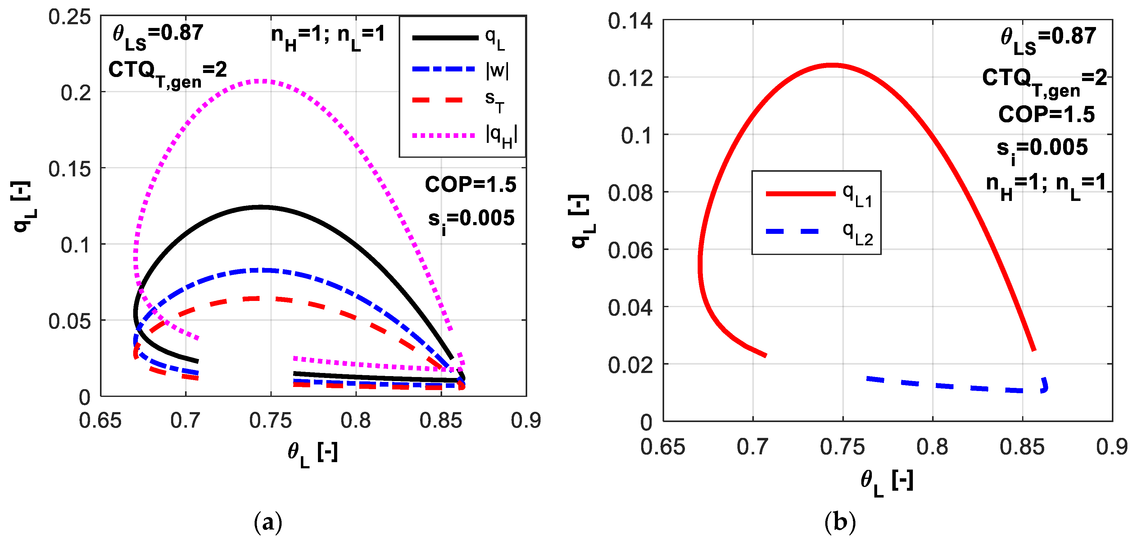
3.1. Imposed Coefficient of Performance
For the numerical simulation, it’s value has been set to COP = 1.5 and for the internal entropy production s̃i = 0.005 was considered. After solving the system of equations, two physical solutions θL and θH are obtained. These two solutions correspond to two different operating regimes, namely one of maximum refrigerating load, denoted by subscript 1, and the other leading to minimum total entropy production, denoted by subscript 2 in the figures. As it was analytically proved, the extrema in both regimes correspond to the same optimum values of system parameters. Results are further presented for the case of linear and non-linear heat transfer laws.
3.1.1. Linear Heat Transfer Laws
In Figure 2a, non-dimensional energy rates and total entropy production are presented for the two operating regimes function on the control variable θL. The upper part of the plots corresponds to the maximum refrigerating load regime, while the lower one corresponds to the minimum total dissipation regime. One might notice that the most convenient operating parameters are those located in the left part of the maximum values, since here the consumed power and total dissipation are lower for lower cold source temperatures.
The non-dimensional refrigerating load is plotted versus θL generating loop curves as shown in Figure 2b. One chosen value for the refrigerant temperature θL might indicate the operation at two refrigerating loads, on the upper part and the lower one respectively
Also, one desired value of the refrigerating load could be associated to a refrigerating temperature closer to the reference one (ambient) as seen in the right-hand-side of the plot, or contrary to a lower temperature value in the left-hand-side. The choice of the operating regime depends on the system settings and the other variables that are behind (θH, CTQL,gen, etc).
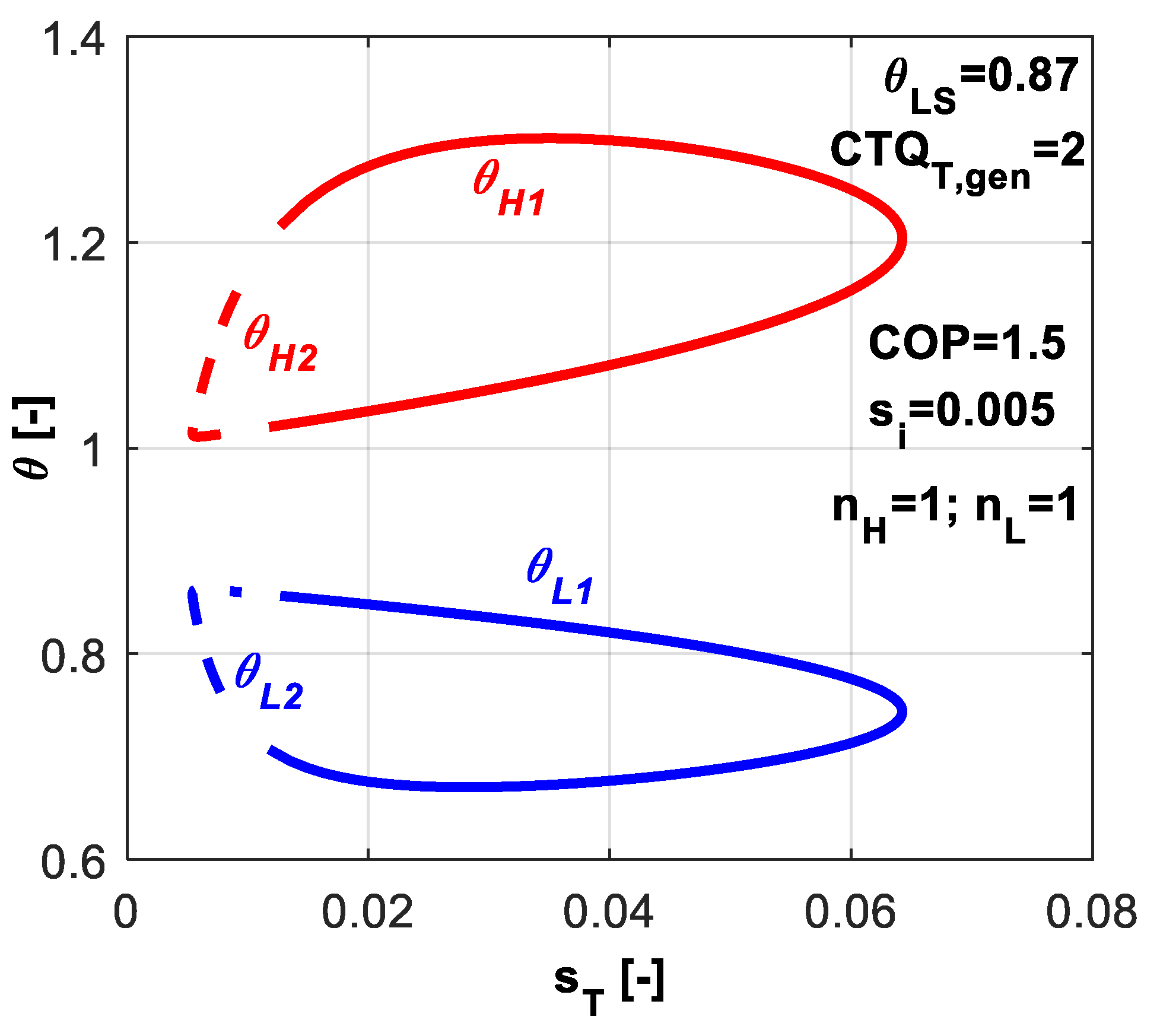
Figure 3 presents a T-s like diagram. The possible range values are emphasized for the refrigerant temperatures at the hot and cold reservoirs. Also one might notice that the second solution of the system of equations (θL2, θH2) corresponds to the lower dissipation rates, but also to the lower energy rates. Thus, the second solution might not be of interest from the operation regime point of view.
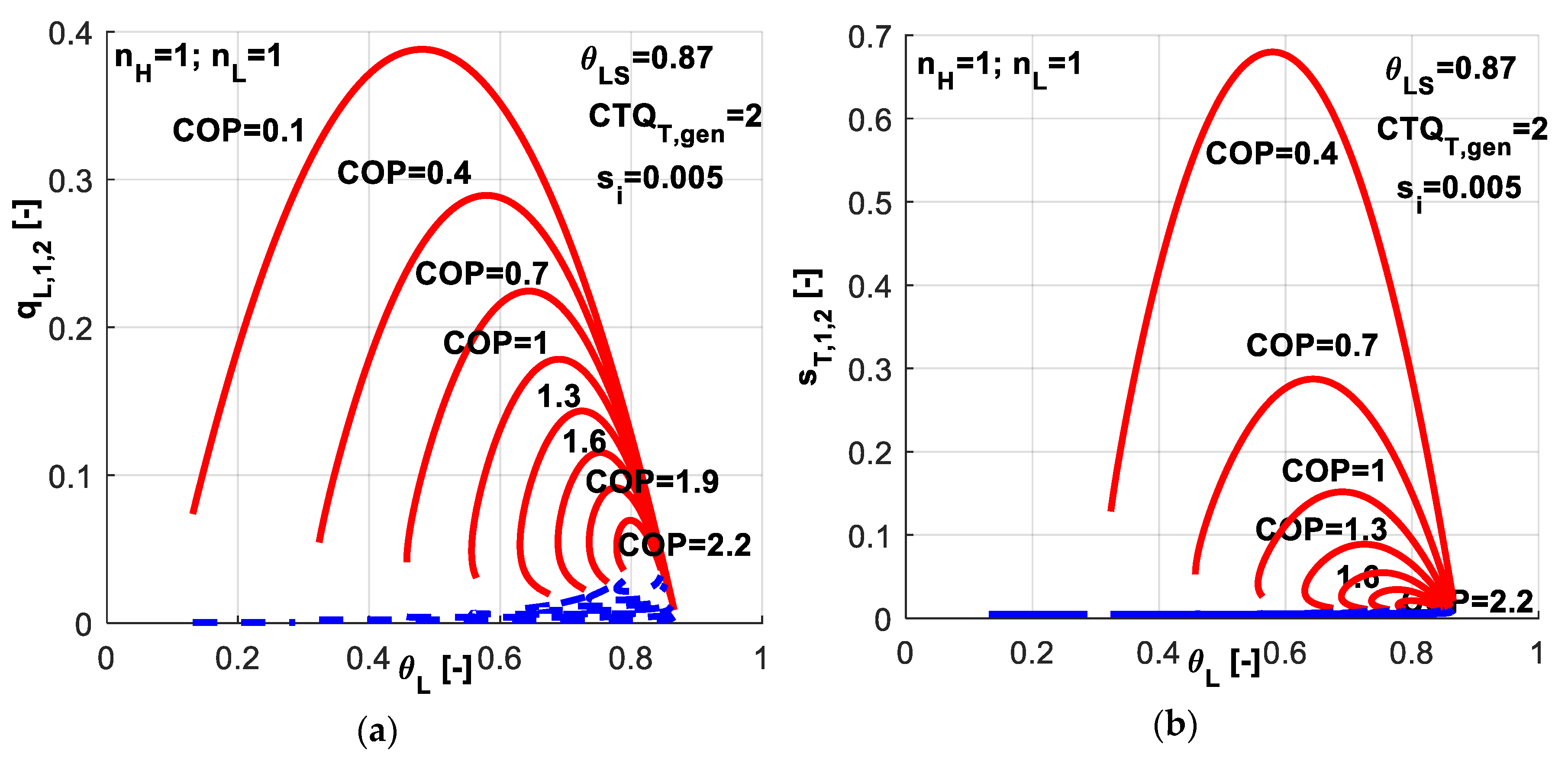
A sensitivity study with respect to COP was performed. It revealed the possible range for system variables and the associated performances. For the maximum refrigeration load regime, as higher COP values constraint the operation, as lower the refrigerating loads are and the range for refrigerant temperature becomes narrower, as emphasized by red upper curves in Figure 4a. For the minimum total dissipation regime (blue down curves in Figure 4a), the higher COP is imposed, the higher refrigerating load is. This particular behavior of the system is explained by the refrigerant temperature variation and heat exchanger inventory distribution in terms of CTQL,gen and CTQH,gen associated to this solution of the equations system. Also one might notice that when the system operates at an imposed COP value, there is a certain refrigerant temperature θL leading to a maximum value of the refrigerating load. The corresponding total entropy production is presented in Figure 4b.
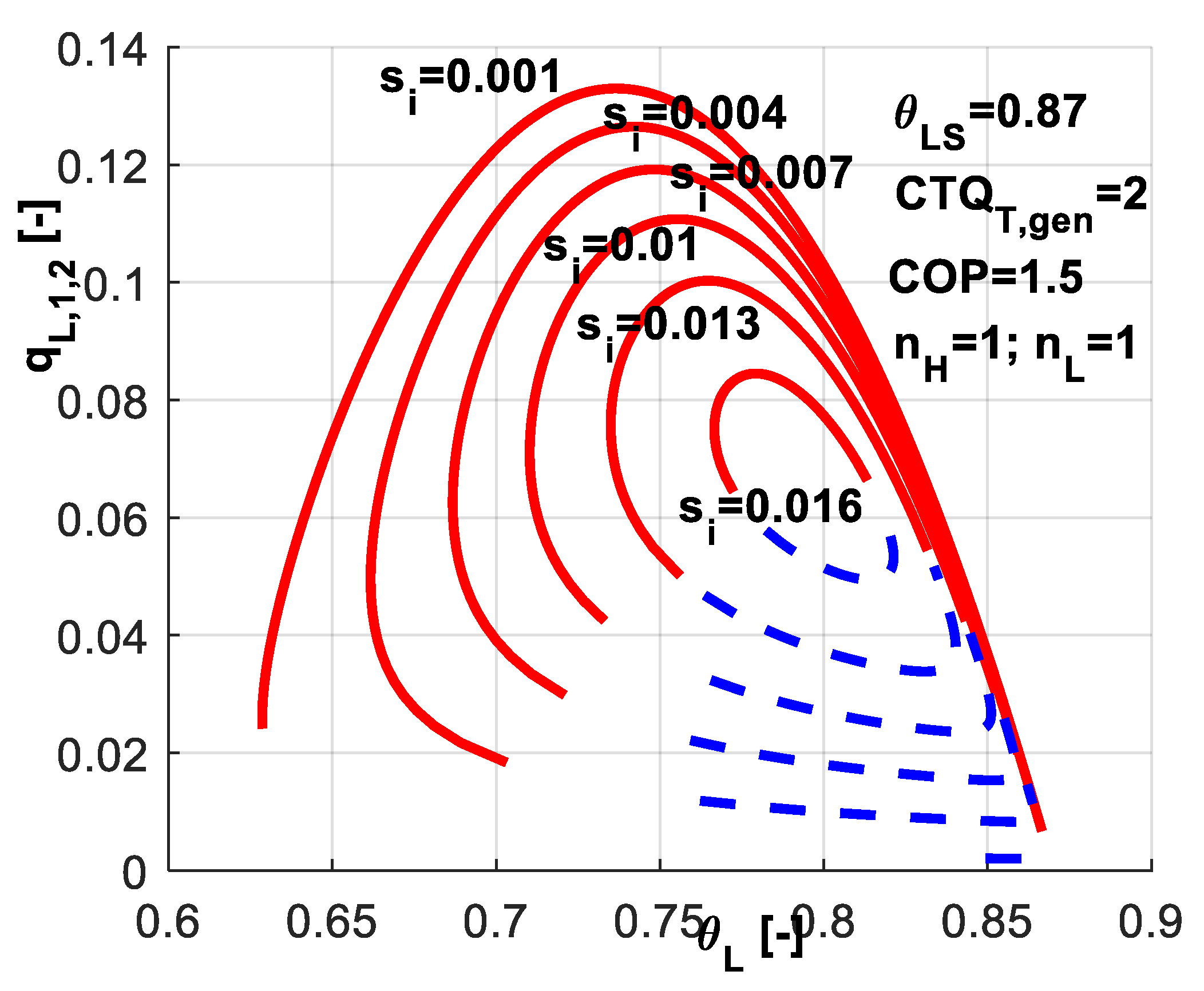
The effect of internal entropy rate s̃i on system variables and performances was studied, too. Its value is closely related to the built machine. Figure 5 reveals that higher s̃i values are accompanied by a narrower range for system variables and obviously lower performances. It is interesting to notice that when operating at higher values of the refrigerant temperature θL, the effect of s̃i is more reduced as emphasized by the curves tangent region in the right-hand-side of the plot. Contrary, its effect is very important in the region of lower refrigerant temperatures—left-hand-side of the curves.
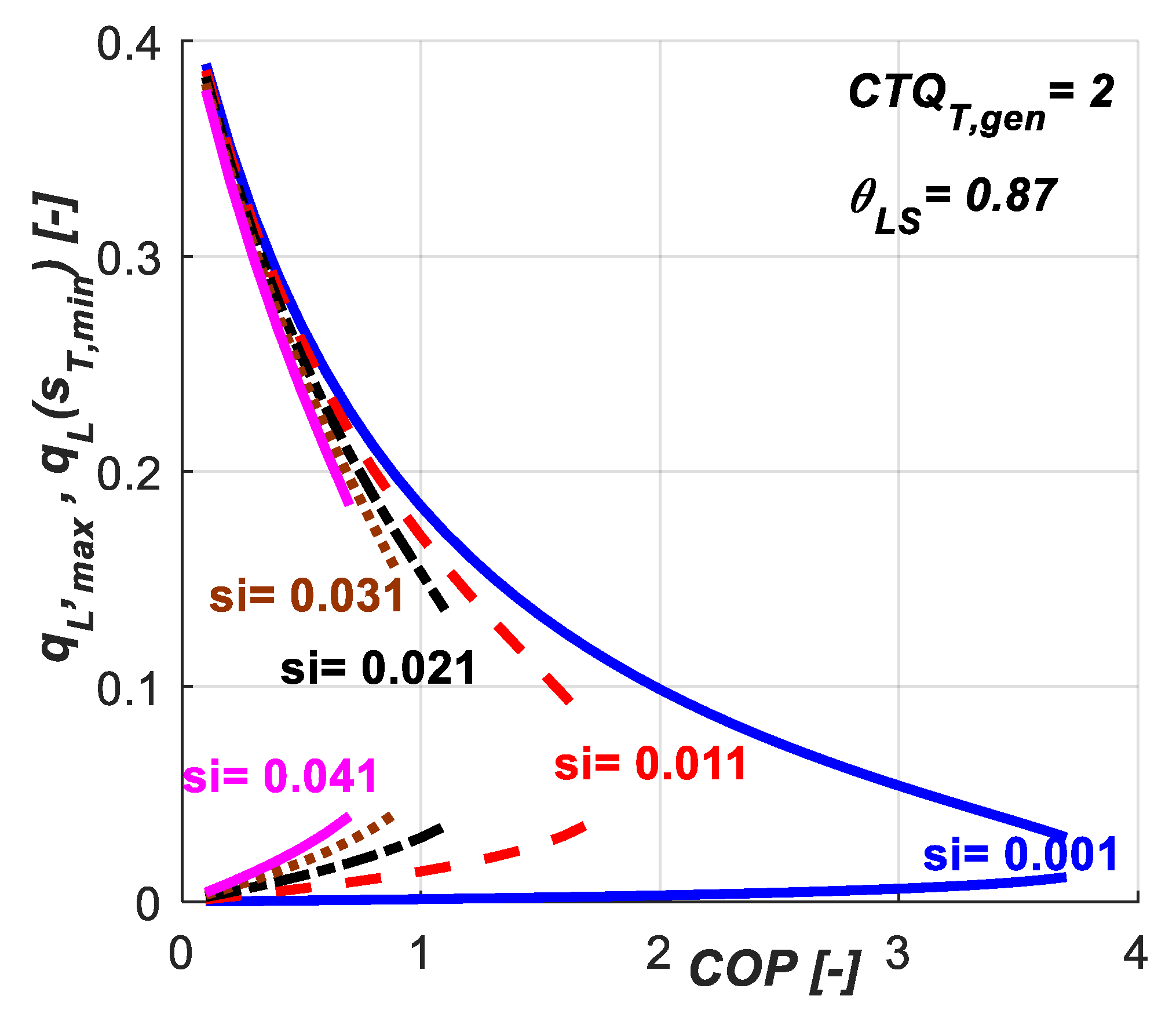
Figure 6 presents the maximum values for the refrigeration load that could be achieved for a given set of COP and s̃i values. It also emphasizes the effect of s̃i on the possible operating range of the system under these constraints. Lower s̃i values let the system operates on a wider range of COP values. Increasing s̃i values limits the system performances in terms of achievable COP and, diminishes the maximum refrigeration load attainable limit (the upper curves) for a given COP value.
3.1.2. Non-Linear Heat Transfer Laws
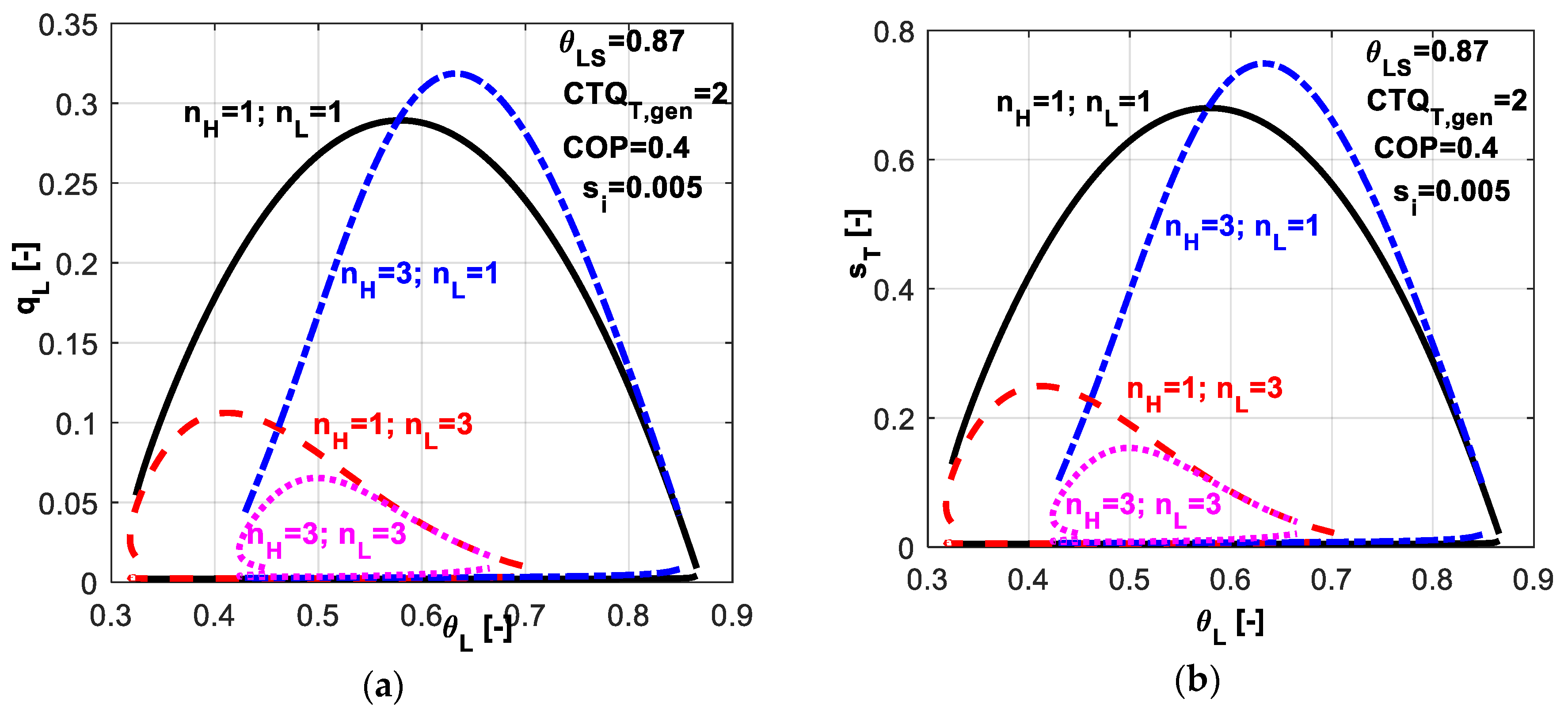
In Figure 7, one might analyze the effect of different nature of heat transfer laws at the source and sink on the non-dimensional refrigerating load (Figure 7a) and total entropy production (Figure 7b). Symmetric and non-symmetric combinations of exponents nH and nL have been chosen. The value of 3 corresponds to a phase change process. The nature of the considered heat transfer laws affects the optimum values of system parameters for obtaining maximum system performances and also the magnitude of system performances.
As revealed by Figure 7a, a phase change process at the cold source (nL = 3) involves lower refrigerating loads and shifts the maximum achievable one towards lower temperature values; the peak of the curves is shifted towards left with respect to the linear case (nH = nL = 1). By constraining the operation at a COP value of 0.4 leads to a maximum achievable non-dimensional refrigerating load of about 0.28 in the case of linear heat transfer laws, and 0.06 respectively for the case of phase change processes at both reservoirs. The justification relies on the temperature difference between the two heat sources and the refrigerant that also depends on the heat transfer law, becoming lower for the phase change processes. We also notice that the nature of the heat transfer law influences the range for possible values of the system variables, especially in the case of phase-change processes.
A sensitivity study with respect to COP values associated to different combinations of heat transfer laws emphasize the results obtained in Figure 8. One might notice that the different considered combinations of exponents nH and nL lead to different possible ranges for COP as a constraint. Maintaining the same settings for the machine as previously (CTQT,gen = 2, θLS = 0.87, s̃i = 0.005), one observes that:
- in the case of linear heat transfer laws at both reservoirs, the COP values could be imposed up to a maximum value of 2.2 (Figure 4);
- when a phase change process in considered at the cold source (Figure 8a,b), the maximum possible COP is about 0.9;
- if the phase change process in considered at the hot sink (Figure 8c,d), the maximum possible COP is about 1.1;
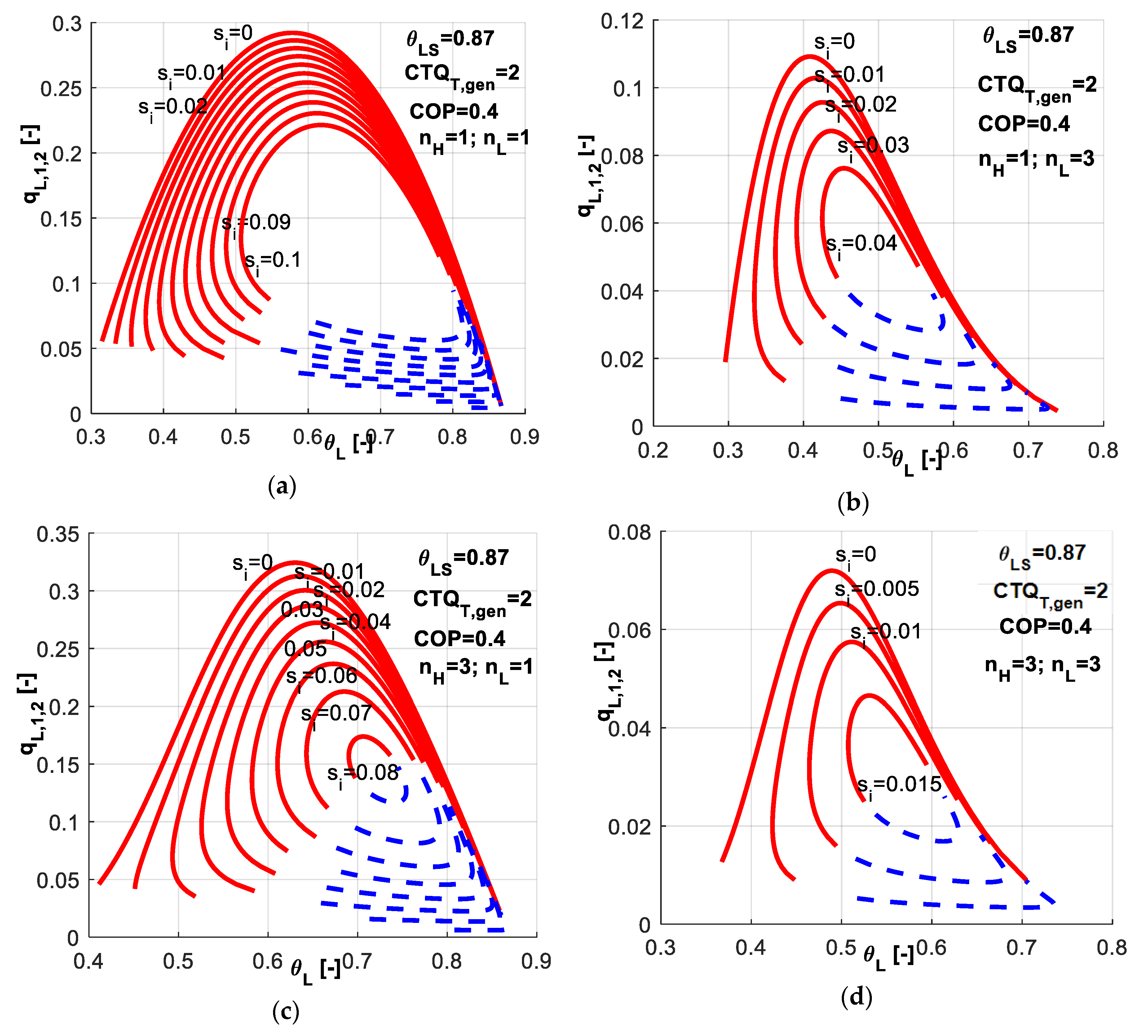
Figure 9 presents the combined effect of heat transfer laws and s̃i constraint values on the non-dimensional refrigerating load and possible range values of refrigerant cold temperature. The first observation regards the s̃i constraint values. Linear heat transfer laws allow the system to operate at higher internal irreversibilities (Figure 9a) when needed, while a phase change process occurring at a heat source limits the operation to lower internal irreversibilities (Figure 9b,c). The most restrictive case is the one at which phase change processes occur at both reservoirs (Figure 9d), for which the maximum acceptable constraint in terms of s̃i is about 0.015 under the other given settings (CTQT,gen, θLS). The second observation refers to the range of achievable θL values. The limit case of endoreversible operation (s̃i = 0) is obviously the most generous in all cases, while the most restrictive one is the case of phase change processes occurring at both reservoirs. For a given value of s̃i = 0.04 for example, the linear case allows θL to be obtained from 0.4 to 0.9 (Figure 9a). When phase change occurs at the cold source (Figure 9b), θL is limited to the range 0.42–0.58, while if the phase change occurs at the hot sink (Figure 9c), the range is 0.55–0.81. The four combinations of heat transfer laws (Figure 9d) do not allow at all the system operation in this case.
The above results contribute to the understanding of the system limits in operation under different constraints and allow the engineer to choose the most convenient variables in certain circumstances.
3.2. Imposed Refrigeration Load
Similar to the previous case, a numerical simulation was carried out when imposing the refrigeration load instead of COP. The considered imposed values for the non-dimensional parameters are q̃L = 0.1 and s̃i = 0.005. The other parameters have the same values, namely θLS = 0.87 and CTQT,gen = 2.
This time the system of equations reveals only one physical solution θL and θH. This solution corresponds to maximum COP operating regime and in the same time to minimum total entropy production one, as proved before (the extrema in both regimes correspond to the same optimum values of system parameters). Results are further presented for the case of linear and non-linear heat transfer laws.
3.2.1. Linear Heat Transfer Laws
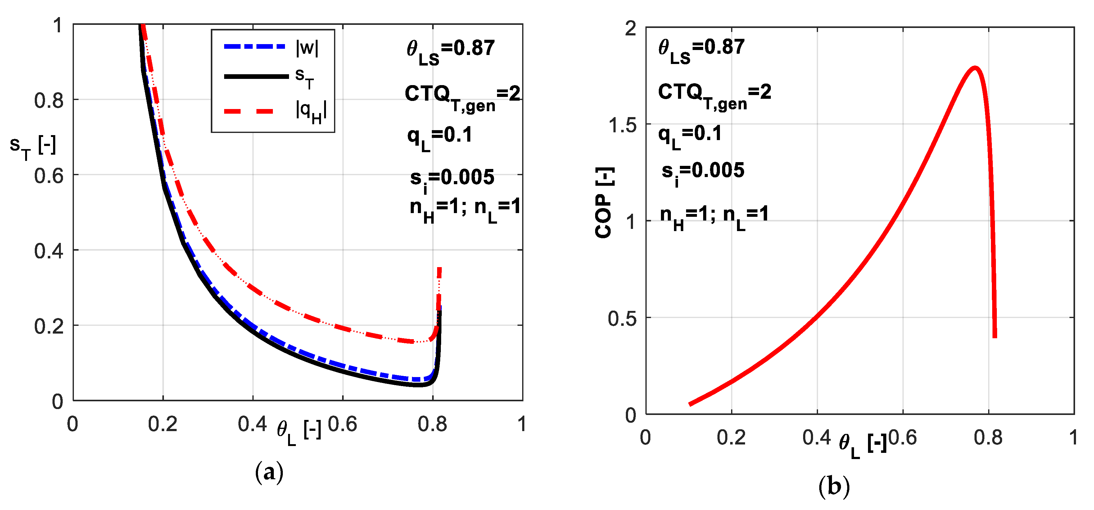
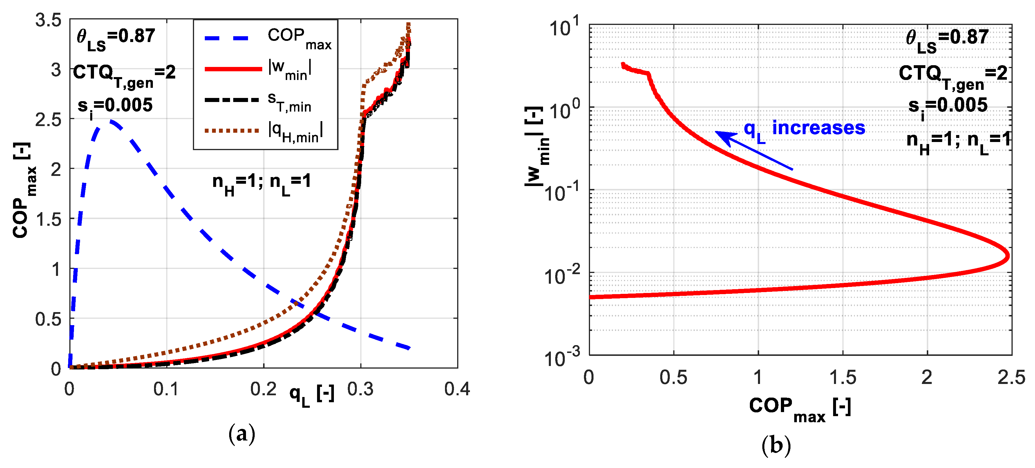
For the case of linear heat transfer laws, the results are plotted in Figure 10. One might notice a large range for the refrigerant cold non-dimensional temperature θL and the existence of an optimum value corresponding to minimum non-dimensional power consumption w̃ and minimum total entropy production s̃T (Figure 10a). This optimum value leads also to maximum COP as revealed by Figure 10b. Numerically, this point tends to equal distribution of CTQ between sources, namely CTQL,gen = CTQH,gen. The results are similar to the previous case where the imposed value of COP leads to an optimum value of θL corresponding to maximum q̃L.
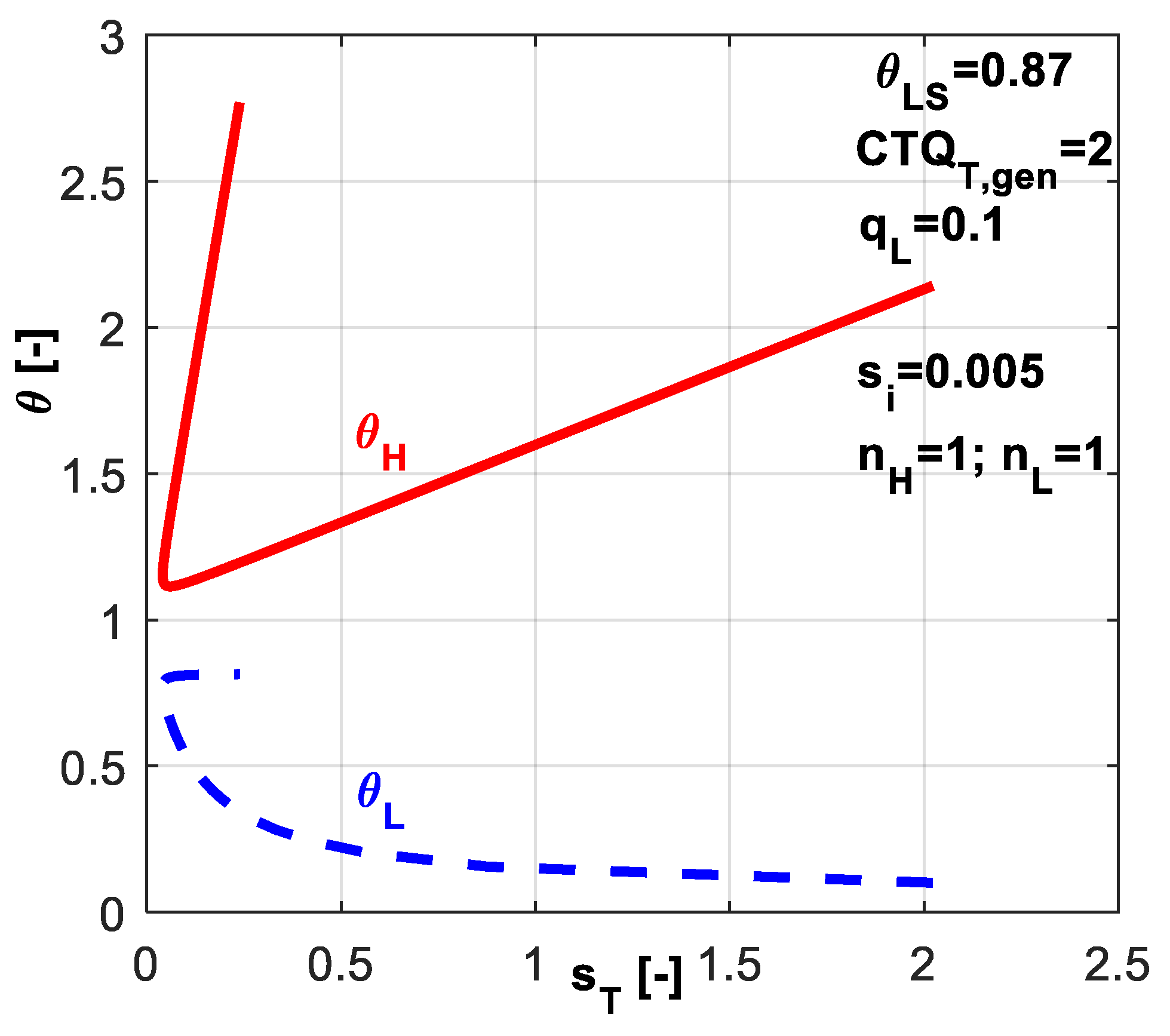
In Figure 11, the non-dimensional temperatures θL and θH are plotted versus dimensionless total entropy production s̃T. Obviously, the cycle operating between minimum difference in refrigerant temperatures is accompanied by the minimum total dissipation (left extrema in Figure 11). As this difference increases, the total dissipation increases.
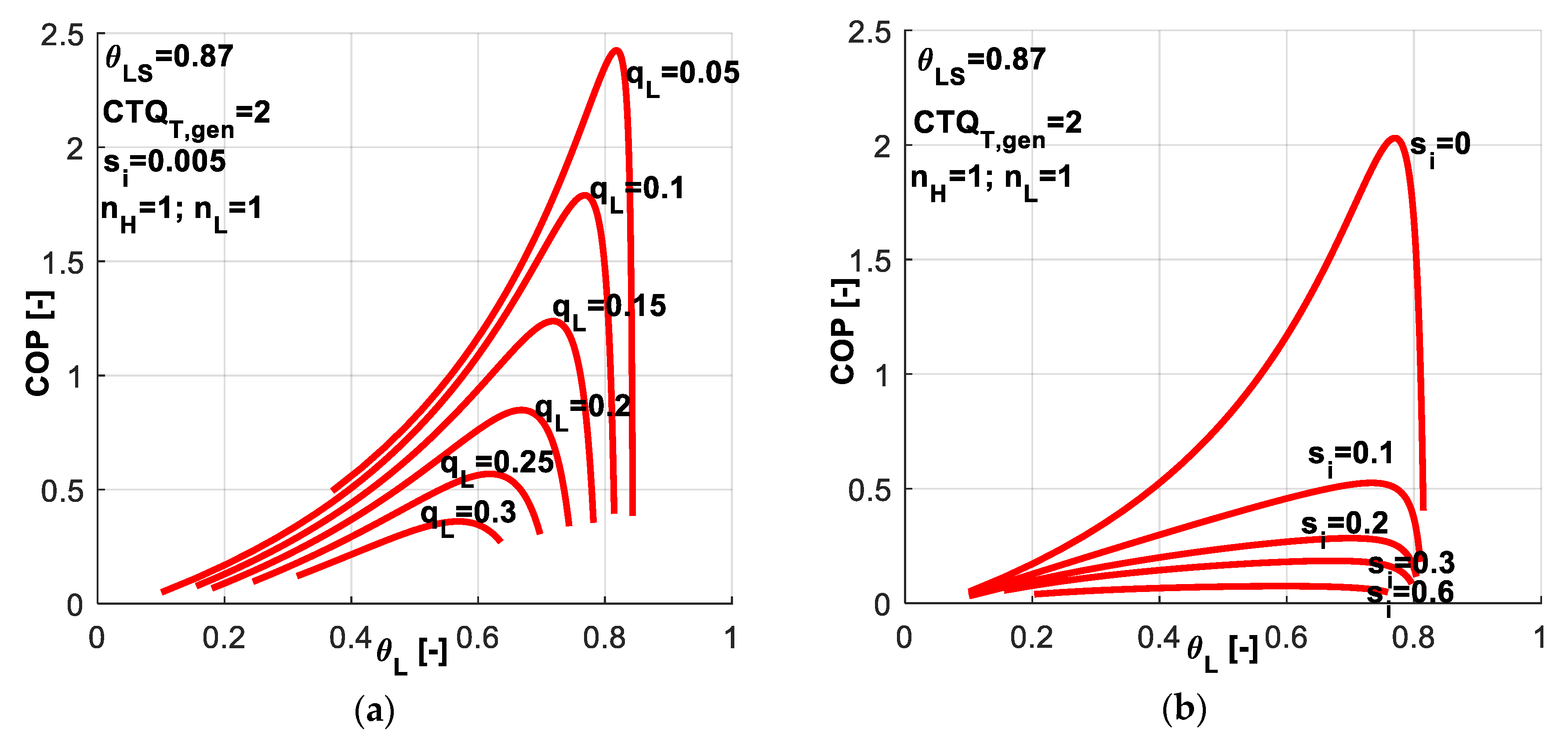
A sensitivity study with respect to the refrigerating load emphasizes the variation range for dimensionless cold refrigerant temperature θL limiting the values of COP (Figure 12a). The behavior is similar to the one presented for the previous case in Figure 4a limiting the values of q̃L when imposing COP. For each imposed q̃L value, an optimum θL value exists for which the system COP is maximum. Higher values of constraint refrigeration load q̃L diminishe the COP values and shift the maximum COP towards lower cold refrigerant temperature values θL. For the chosen set of system parameters, a dimensionless refrigeration load of 0.3 is the maximum attainable in the range of 0.35–0.62 for θL values. The internal entropy production effects are emphasized in Figure 12b. The most important effect is noticed on limiting the COP values, rather than limiting θL.
Figure 13 presents the variation of maximum COP values and the corresponding minimum energy rates and total entropy dissipation with dimensionless refrigerating load. A maximum value among the COP maxima is obtained for q̃L = 0.04 in the given conditions. These types of plots could be used to set the system operating regimes for maximum performances under some imposed constraint. Figure 13b emphasizes the variation of dimensionless consumed mechanical power with maximum COP, at logarithmic scale, for increasing q̃L values. This plot puts into evidence that the chosen operating regime is a trade-off between COP and refrigerating load q̃L, for high value of q̃L. The lower part of the curve corresponds to low values of q̃L and w̃, and the value of maximum COP appears as a transition point.
3.2.2. Non-Linear Heat Transfer Laws
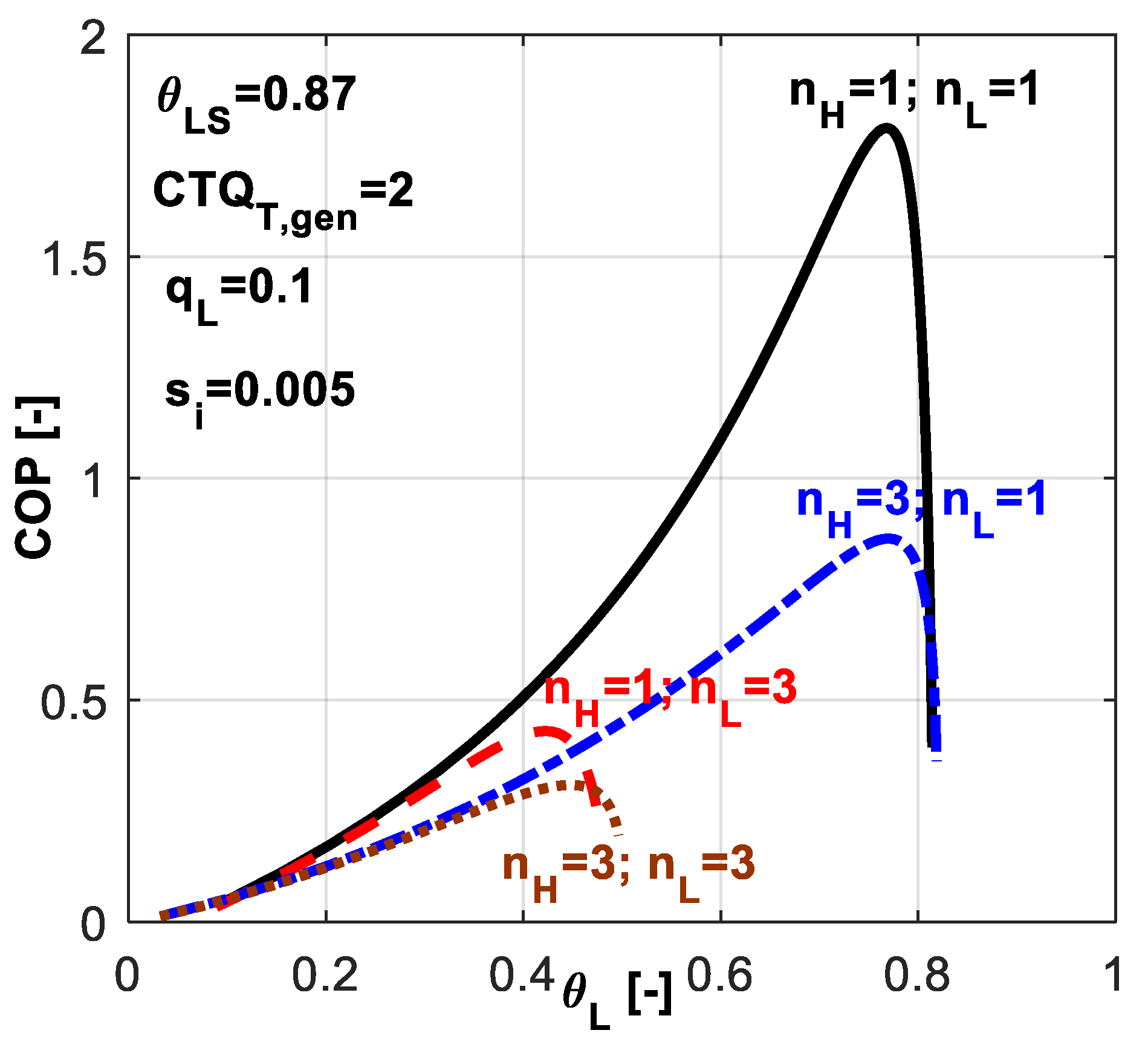
The effect of different combinations of heat transfer laws on the system COP is emphasized in Figure 14. The most favorable combination from COP point of view is the case of linear heat transfer laws at both sides, while the most constrainable is the one considering phase change processes at both sides. These two combinations constraint the COP values and also the range for allowable θL values.
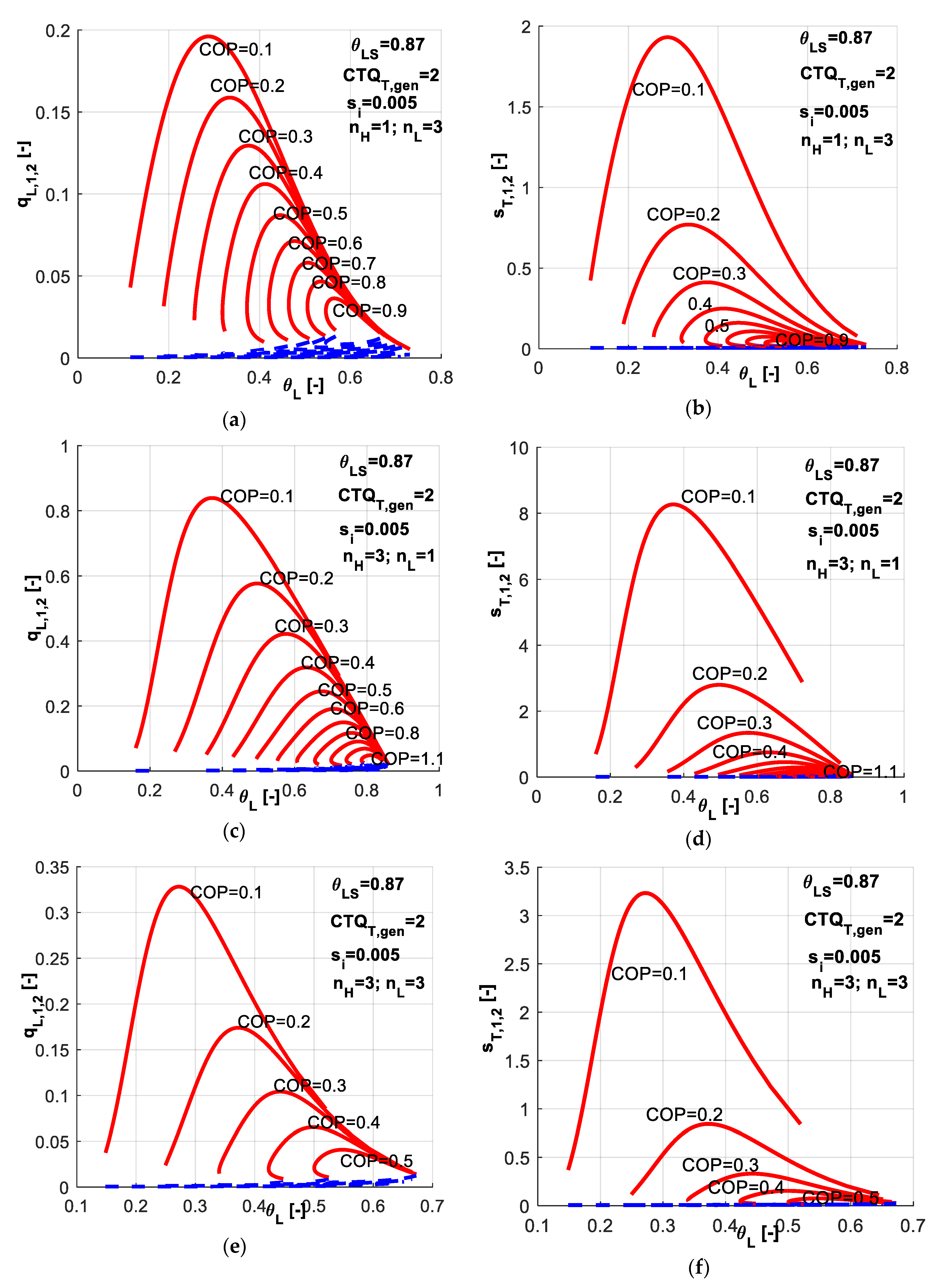
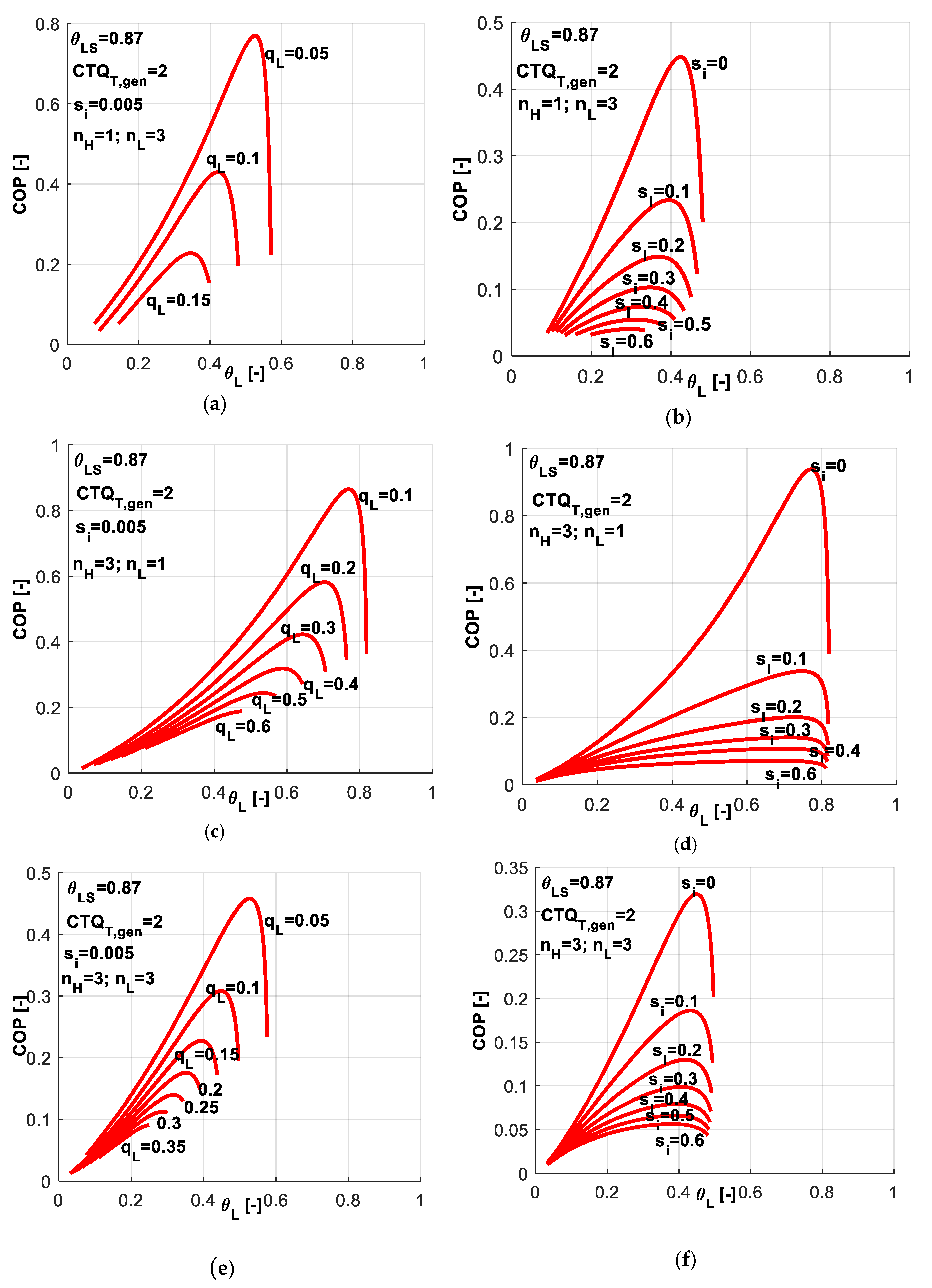
Figure 15 presents a sensitivity study with respect to q̃L and s̃i values associated to different combinations of heat transfer laws. This study is similar to the one presented in Figure 8 when imposing COP instead of q̃L. One might notice that the different considered combinations of exponents nH and nL lead to different possible ranges for q̃L as a constraint and for θL as control variable. Maintaining the same settings for the machine in all cases (CTQT,gen = 2, θLS = 0.87, s̃i = 0.005), one observes that:
- in the case of linear heat transfer laws at both reservoirs, the q̃L values could be imposed up to a maximum value of about 0.3 (Figure 12a); the limits in θL are quite large and the θL values are naturally decreasing as q̃L decreases;
- when a phase change process in considered at the cold source (Figure 15a,b), the maximum possible q̃L is about 0.15, half of the above-mentioned value; also the limits for θL values are much reduced;
- if the phase change process in considered at the hot sink (Figure 15c,d), the maximum possible q̃L is about 0.6, so twice with respect to the linear case; the limits for θL values are comparable to those obtained for the linear case;
- while in the case of phase change process at both reservoirs (Figure 15e,f), the q̃L is limited to 0.35, and thus the effects of the two phase change processes are cancelling each other when comparing to the linear laws; θL values are more reduced in this case.
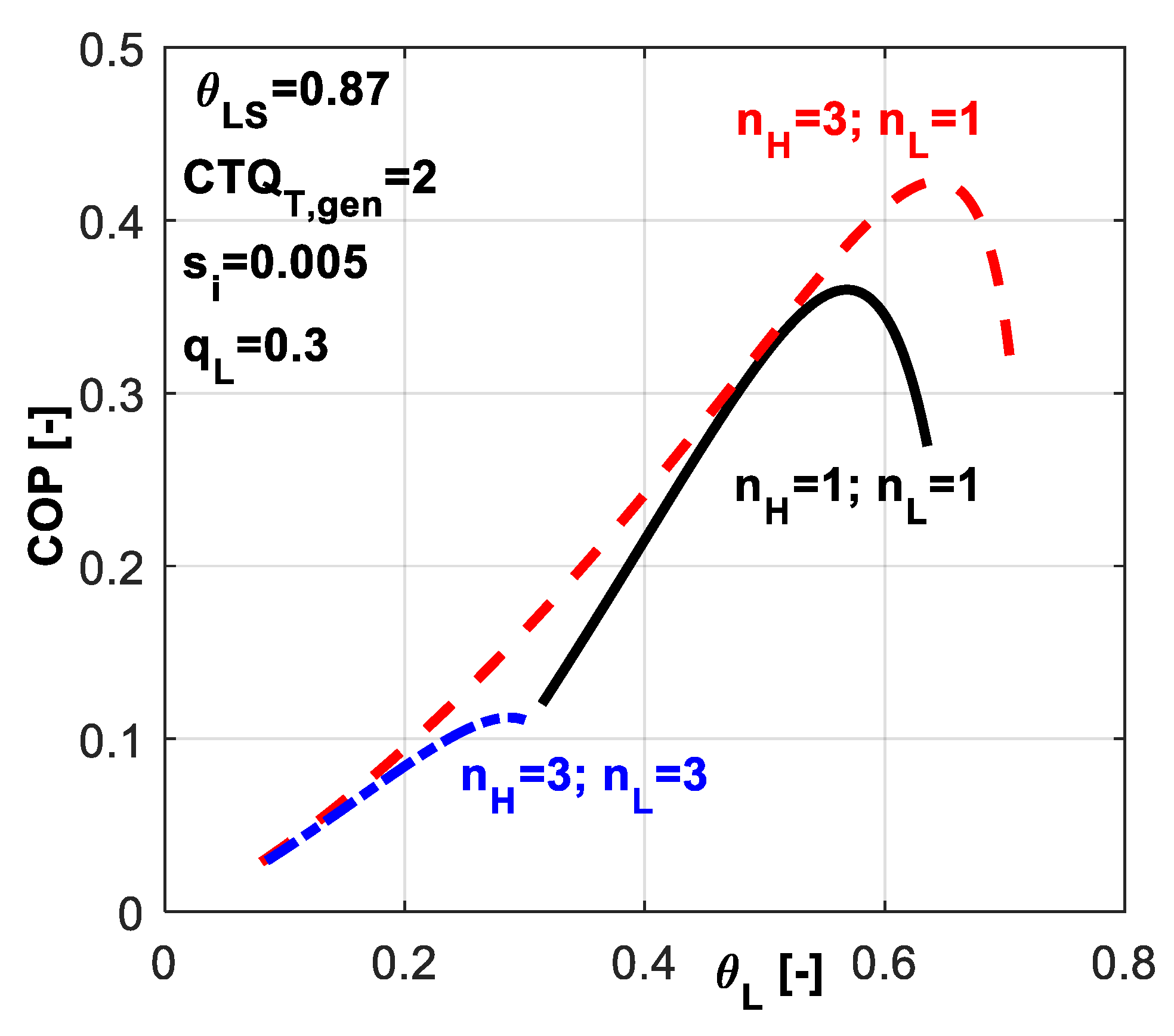
One might deduce from these results that when a system is supposed to undergo a deep cooling process, the nature of the heat transfer law is very important. In this regard, Figure 16 reveals the effect of chosen heat transfer law for such applications, when the required dimensionless refrigerating load is more important, here q̃L = 0.3.
One might notice that for this application, the best alternative is to choose a linear heat transfer law at the sink and a phase change process at the hot source (nH = 3, nL = 1). This combination leads to maximum COP for a required cold temperature and also it allows the system operation over a wider range of θL values. From Figure 15c one may also notice that this combination ensures the system operation at heavier refrigerating loads.
4. Conclusions and Perspectives
A general model for the study and optimization of irreversible refrigeration Carnot-like machines was presented. The study started with machines optimization under different constraints and ended with important aspects related to the intrinsic phenomena affecting the systems operation.
The results confirm that the First and Second Law of Thermodynamics are very useful tools in optimization problems under constraints.
The system limits in operation under different constraints were emphasized from the point of view of possible values for system control variables (such as θL), for imposed constraint (COP or q̃L) and achievable performances (q̃L or COP, s̃T, other dimensionless energy rates). Moreover, the results are useful in deciding the most convenient values and heat transfer laws in particular circumstances and for specific applications.
The above results contribute to the understanding of the system limits in operation under different constraints and allow the engineer to choose the most convenient variables in given circumstances.
Optimal variables are found for the best performances that the system could achieve under specified constraints. Also the limits of the system operation are determined.
Further development of the model for other constraints (imposed w̃ or q̃H) is in progress. Also, a comparison of the direct and reverse machine models and results are under consideration. It seems very promising and gives a new perspective on their optimization through a unitary approach.
Author Contributions
C.S. contributed to the development of the model, design of the study and Matlab programming; M.F. contributed to the state of the art analysis and development of the methodology; M.C. contributed to the preparation of the manuscript and final proof and to the analysis and interpretation of the results; D.S. contributed to the Matlab programming and analysis and interpretation of the results.
Funding
This research received no external funding.
Conflicts of Interest
The authors declare no conflict of interest. The funders had no role in the design of the study; in the collection, analyses, or interpretation of data; in the writing of the manuscript, or in the decision to publish the results.
List of Symbols
| A | heat transfer area, [m2] |
| COP | coefficient of performance, [-] |
| CTQgen | generalized number of heat transfer units, [-] |
| f, g | functions defined in the model |
| Kgen | generalized conductance, [W K−n] |
| heat rate capacity, [W K−1] | |
| n | exponent of the heat transfer law, [-] |
| heat transfer rate, [W] | |
| dimensionless heat transfer rate, [-] | |
| entropy production, [W K−1] | |
| dimensionless entropy production, [-] | |
| T | temperature, [K] |
| U | overall heat transfer coefficient, [W m−2 K−1] |
| mechanical power, [W] | |
| w̃ | dimensionless mechanical power, [-] |
| Greek Symbols | |
| λ | Lagrange multiplier |
| θ | non-dimensional temperature |
| ξ | function defined in the model |
| Subscript | |
| gen | generalized |
| H | working fluid, at the machine hot temperature side |
| HS | source, at the machine hot temperature side |
| i | internal |
| L | working fluid, at the machine low temperature side |
| LS | source, at the machine low temperature side |
| T | total |
| Abbreviations | |
| C | constraint |
| FO | objective function |
| L | Lagrangian function |
References
- Novikov, I. The efficiency of atomic power stations. Atommaya Energiya 1957, 3, 409. [Google Scholar]
- Chambadal, P. Évolution et Applications du Concept D’entropie; Dunod: Paris, France, 1963. (In French) [Google Scholar]
- Curzon, F.L.; Ahlborn, B. Efficiency of a Carnot Engine at Maximum Power Output. Am. J. Phys. 1975, 43, 22–24. [Google Scholar] [CrossRef]
- De Vos, A. Efficiency of some heat engines at maximum power conditions. Am. J. Phys. 1985, 53, 570–573. [Google Scholar] [CrossRef]
- Salamon, P.; Nitzan, A. Finite Time optimizations of a Newton’s law Carnot cycle. J. Chem. Phys. 1981, 74, 3546–3560. [Google Scholar] [CrossRef]
- Blanchard, C.H. Coefficient of performance for finite speed heat pump. J. App. Phys. 1980, 51, 2471–2472. [Google Scholar] [CrossRef]
- Goth, Y.; Feidt, M. Recherche des conditions optimales de fonctionnement des pompes à chaleur ou machines à froid asociées à un cycle de Carnot endoréversible. C. R. Acad. Sci. 1986, 303, 113–122. (In French) [Google Scholar]
- Feidt, M. Optimization of thermal systems and processes, application to heat pumps. In Proceedings of the ICIAM’87 Conference, Paris, France, 29 June–3 July 1987. [Google Scholar]
- Feidt, M. Finite Time Thermodynamics applied to optimization of heat pump and refrigerating machines cycles. In Proceedings of the 12th IMACS World Congress on Scientific Computation, Paris, France, 18–22 July 1988. [Google Scholar]
- Boussehain, R.; Feidt, M. Cycle optimization for a refrigeration system with three heat reservoirs. In Proceedings of the Séminaire Franco-Allemand, Kasel, Germany, 1–4 October 1984. [Google Scholar]
- Feidt, M. Un outil d’aide à la conception des machines à froid et pompes à chaleur à partir de la modélisation des cycles des machines à deux et trois sources de chaleur. Optimisation résultante compte tenu de contraintes en temps de cycle ou en surface d’échange. In Proceedings of the Rencontre S.F.T.’86, Marseille, France, 5–7 May 1986. (In French). [Google Scholar]
- Boussehain, R.; Feidt, M. Optimisation théorique du cycle d’une machine à froid endoréversible à trois sources de chaleur. In Proceedings of the 1st Magrbian Colloque on the Engineering Numerical Models, Alger, Algeria, 22–23 November 1987. (In French). [Google Scholar]
- Feidt, M. Thermodynamics and optimization of reverse cycle machines: Refrigeration, heat pumps, air conditioning, cryogenics. In Thermodynamics Optimization of Complex Energy Systems; Bejan, A., Mamut, E., Eds.; Kluwer Academic Publishers: Dordrecht, The Netherlands, 1999; pp. 385–401. [Google Scholar]
- Feidt, M. Thermodynamics applied to reverse cycle machines, a review. Int. J. Refrig. 2010, 33, 1327–1342. [Google Scholar] [CrossRef]
- Feidt, M. Evolution of thermodynamics modeling for three and four heat reservoirs reverse cycle machines: A review and new trends. Int. J. Refrig. 2013, 36, 8–23. [Google Scholar] [CrossRef]
- Assad, M. Performance characteristics of an irreversible refrigerator. In Recent Advanced in Finite Time Thermodynamics; Nova Science Publishers: New York, NY, USA, 2000. [Google Scholar]
- Feidt, M. Advanced Thermodynamics of reverse cycle machine. In Low Temperature and Cryogenic Refrigeration; Kluwer Academic Publishers: Dordrecht, The Netherlands, 2003. [Google Scholar]
- Medjo Nouadje, B.A.; Ngouateu Wouagfack, P.A.; Tchinda, R. Influence of two internal irreversibilities on the new thermo-ecological criterion for three-heat-source refrigerators. Int. J. Refrig. 2014, 38, 118–127. [Google Scholar] [CrossRef]
- Sieniutycz, S.; Salamon, P. Finite-Time Thermodynamics and Thermoeconomics; Taylor & Francis: New York, NY, USA, 1990. [Google Scholar]
- Calvo Hernández, A.; Medina, A.; Roco, J.M.M.; Velasco, S. Comparison of Optimum Thermal Conductance Distribution for an Irreversible Carnot Cycle under Different Optimization Criteria. In Advances in Finite Time Thermodynamics, Analysis and Optimization; Nova Science Publishers: New York, NY, USA, 2004. [Google Scholar]
- Petrescu, S.; Zaiser, J.; Petrescu, V. Lectures on Advanced Energy Conversion; Bucknell: Lewisburg, PA, USA, 1996. [Google Scholar]
- Bejan, A. Entropy Generation Minimization; Wiley & Sons: New York, NY, USA, 1982. [Google Scholar]
- Feidt, M. Thermodynamique et Optimisation Energétique des Systèmes et Procédés; Tech. & Doc.: Paris, France, 1996. (In French) [Google Scholar]
- Petrescu, S.; Costea, M. Development of Thermodynamics with Finite Speed and Direct Method; AGIR: Bucharest, Romania, 2011. [Google Scholar]
- Bejan, A. Advanced Engineering Thermodynamics; Wiley & Sons: New York, NY, USA, 1988. [Google Scholar]
- Petrescu, S.; Costea, M.; Feidt, M.; Ganea, I.; Boriaru, N. Advanced Thermodynamics of Irreversible Processes with Finite Speed and Finite Dimensions. A Historical and Epistemological Approach, with Extension to Biological and Social Systems; AGIR: Bucharest, Romania, 2015. [Google Scholar]
- Berrich Betouche, E.; Fellah, A.; Ben Brahim, A.; Aloui, F.; Feidt, M. Thermodynamic Analysis of the Irreversibilities in Solar Absorption Refrigerators. Entropy 2016, 18, 107. [Google Scholar] [CrossRef]
- Petre, C.; Feidt, M.; Costea, M.; Petrescu, S. Model général de machine de Carnot à cycle inverse soumise à diverses contraintes de fonctionnement. In Proceedings of the XIVth National Conference on Thermodynamics, SRT 2004; Technical University of Civil Engineering: Bucharest, Romania, 2004. [Google Scholar]
- Petre, C.; Feidt, M.; Petrescu, S.; Costea, M. Thermodynamique en dimensions finies. Optimisation de la machine de Carnot a cycle inverse irreversible avec puissance frigorifique imposée. In Proceedings of the XVth National Conference on Thermodynamics SRT 2005; Technical University of Craiova: Craiova, Romania, 2005. [Google Scholar]
- Feidt, M.; Petre, C.; Costea, M.; Petrescu, S. General Model of Reversed Cycle Carnot Machine with Contraints and Non-Linear Heat Transfer Laws. In Proceedings of the 18th International Conference on Efficiency, Cost, Optimization, Simulation and Enviromental Impact of Energy Systems, ECOS 2005, Trondheim, Norwey, 20–22 June 2005. [Google Scholar]
- Petre, C. Finite-Speed Thermodynamics Use in the Study and Optimization of Carnot Cycle and Stirling Machines. Ph.D. Thesis, University Politehnica of Bucharest, Romania – University “Henri Poincaré”, Nancy, France, 2007. (In Romanian). [Google Scholar]
- Qureshi, B.A.; Zubair, S.M. Thermoeconomic considerations in the allocation of heat transfer inventory for irreversible refrigeration and heat pump systems. Int. J. Refrig. 2015, 54, 67–75. [Google Scholar] [CrossRef]
- Sarbu, I. A review on substitution strategy of non-ecological refrigerants from vapour compression-based refrigeration, air conditioning and heat pump systems. Int. J. Refrig. 2014, 46, 123–141. [Google Scholar] [CrossRef]
- Ngouateu Wouagfack, P.A.; Tchinda, R. Optimal performance of an absorbtion refrigerator based on maximum ECOP. Int. J. Refrig. 2014, 40, 404–415. [Google Scholar] [CrossRef]
- Gordon, J.M.; Ng, K.C. Cool Thermodynamics; Cambridge International Science Publishing: Cambridge, UK, 2000. [Google Scholar]
- Wijeysundera, N.E. Performance of three heat reservoirs absorption cycles with external and internal irreversibilities. Appl. Therm. Eng. 1997, 17, 1151–1161. [Google Scholar] [CrossRef]
Figure 1.
Irreversible Carnot-like refrigeration machine: (a) Scheme; (b) Irreversible cycle in T-S diagram.
Figure 1.
Irreversible Carnot-like refrigeration machine: (a) Scheme; (b) Irreversible cycle in T-S diagram.

Figure 2.
Imposed COP and s̃i constant: (a) Non-dimensional energy rates and total entropy production for the two operating regimes; (b) Non-dimensional refrigerating load for the two operating regimes.
Figure 2.
Imposed COP and s̃i constant: (a) Non-dimensional energy rates and total entropy production for the two operating regimes; (b) Non-dimensional refrigerating load for the two operating regimes.

Figure 3.
The two solutions of the non-dimensional refrigerant temperatures function on s̃T for the case with imposed COP and s̃i constant.
Figure 3.
The two solutions of the non-dimensional refrigerant temperatures function on s̃T for the case with imposed COP and s̃i constant.

Figure 4.
Imposed COP and s̃i constant - sensitivity study with respect to COP (a) Non-dimensional refrigeration load for the two regimes; (b) Non-dimensional total entropy production for the two regimes.
Figure 4.
Imposed COP and s̃i constant - sensitivity study with respect to COP (a) Non-dimensional refrigeration load for the two regimes; (b) Non-dimensional total entropy production for the two regimes.

Figure 5.
Imposed COP and s̃i constant - sensitivity study with respect to s̃i. Non-dimensional refrigeration load for the two regimes.
Figure 5.
Imposed COP and s̃i constant - sensitivity study with respect to s̃i. Non-dimensional refrigeration load for the two regimes.

Figure 6.
Maximum refrigeration load for a given set of COP and s̃i constant values.

Figure 7.
Imposed COP and s̃i constant - sensitivity study with respect to heat transfer laws nature at both reservoirs (a) Non-dimensional refrigerating load; (b) Non-dimensional total entropy production.
Figure 7.
Imposed COP and s̃i constant - sensitivity study with respect to heat transfer laws nature at both reservoirs (a) Non-dimensional refrigerating load; (b) Non-dimensional total entropy production.

Figure 8.
COP and s̃i constant constraints - sensitivity study with respect to heat transfer laws nature at both reservoirs for different combinations (nH, nL).
Figure 8.
COP and s̃i constant constraints - sensitivity study with respect to heat transfer laws nature at both reservoirs for different combinations (nH, nL).

Figure 9.
Imposed COP and s̃i constant – non-dimensional refrigerating load for different combinations of heat transfer laws at both reservoirs (nH, nL).
Figure 9.
Imposed COP and s̃i constant – non-dimensional refrigerating load for different combinations of heat transfer laws at both reservoirs (nH, nL).

Figure 10.
Imposed q̃L and s̃i constant (a) Non-dimensional energy rates and total entropy production; (b) COP variation with respect to θL.
Figure 10.
Imposed q̃L and s̃i constant (a) Non-dimensional energy rates and total entropy production; (b) COP variation with respect to θL.

Figure 11.
Non-dimensional refrigerant temperatures at hot and cold reservoirs for the case of imposed q̃L and s̃i constant.
Figure 11.
Non-dimensional refrigerant temperatures at hot and cold reservoirs for the case of imposed q̃L and s̃i constant.

Figure 12.
COP variation for the case with imposed q̃L and s̃i constant (a) Sensitivity with respect to dimensionless refrigerating load; (b) Sensitivity with respect to dimensionless internal entropy production.
Figure 12.
COP variation for the case with imposed q̃L and s̃i constant (a) Sensitivity with respect to dimensionless refrigerating load; (b) Sensitivity with respect to dimensionless internal entropy production.

Figure 13.
q̃L influence: (a) Dimensionless energy rates and COP variation–sensitivity with respect to q̃L; (b) Dimensionless consumed power versus maximum achievable COP.
Figure 13.
q̃L influence: (a) Dimensionless energy rates and COP variation–sensitivity with respect to q̃L; (b) Dimensionless consumed power versus maximum achievable COP.

Figure 14.
COP variation for the case of imposed q̃L and s̃i constant - sensitivity study with respect to heat transfer laws nature at the source and sink.
Figure 14.
COP variation for the case of imposed q̃L and s̃i constant - sensitivity study with respect to heat transfer laws nature at the source and sink.

Figure 15.
COP variation for the case of imposed q̃L and s̃i constant, for different combinations of heat transfer laws - sensitivity study with respect to q̃L and s̃i.
Figure 15.
COP variation for the case of imposed q̃L and s̃i constant, for different combinations of heat transfer laws - sensitivity study with respect to q̃L and s̃i.

Figure 16.
COP variation for the case of imposed q̃L and s̃i constant - sensitivity study with respect to heat transfer laws nature at the reservoirs.
Figure 16.
COP variation for the case of imposed q̃L and s̃i constant - sensitivity study with respect to heat transfer laws nature at the reservoirs.

© 2018 by the authors. Licensee MDPI, Basel, Switzerland. This article is an open access article distributed under the terms and conditions of the Creative Commons Attribution (CC BY) license (http://creativecommons.org/licenses/by/4.0/).
Share and Cite
MDPI and ACS Style
Stanciu, C.; Feidt, M.; Costea, M.; Stanciu, D. Optimization and Entropy Production: Application to Carnot-Like Refrigeration Machines. Entropy 2018, 20, 953. https://doi.org/10.3390/e20120953
AMA Style
Stanciu C, Feidt M, Costea M, Stanciu D. Optimization and Entropy Production: Application to Carnot-Like Refrigeration Machines. Entropy. 2018; 20(12):953. https://doi.org/10.3390/e20120953
Chicago/Turabian StyleStanciu, Camelia, Michel Feidt, Monica Costea, and Dorin Stanciu. 2018. "Optimization and Entropy Production: Application to Carnot-Like Refrigeration Machines" Entropy 20, no. 12: 953. https://doi.org/10.3390/e20120953
Note that from the first issue of 2016, this journal uses article numbers instead of page numbers. See further details here.