
Spurious Results of Fluctuation Analysis Techniques in Magnitude and Sign Correlations
by
Pedro Carpena
*, 
Manuel Gómez-Extremera
, 
Concepción Carretero-Campos
,
Pedro Bernaola-Galván
and
Ana V. Coronado
Departamento de Física Aplicada II, E.T.S.I. de Telecomunicación, Universidad de Málaga, 29071 Málaga, Spain
*
Author to whom correspondence should be addressed.
Entropy 2017, 19(6), 261; https://doi.org/10.3390/e19060261
Submission received: 10 May 2017
/
Revised: 31 May 2017
/
Accepted: 2 June 2017
/
Published: 7 June 2017
(This article belongs to the Special Issue Complex Systems, Non-Equilibrium Dynamics and Self-Organisation)
Abstract
:Fluctuation Analysis (FA) and specially Detrended Fluctuation Analysis (DFA) are techniques commonly used to quantify correlations and scaling properties of complex time series such as the observable outputs of great variety of dynamical systems, from Economics to Physiology. Often, such correlated time series are analyzed using the magnitude and sign decomposition, i.e., by using FA or DFA to study separately the sign and the magnitude series obtained from the original signal. This approach allows for distinguishing between systems with the same linear correlations but different dynamical properties. However, here we present analytical and numerical evidence showing that FA and DFA can lead to spurious results when applied to sign and magnitude series obtained from power-law correlated time series of fractional Gaussian noise (fGn) type. Specifically, we show that: (i) the autocorrelation functions of the sign and magnitude series obtained from fGns are always power-laws; However, (ii) when the sign series presents power-law anticorrelations, FA and DFA wrongly interpret the sign series as purely uncorrelated; Similarly, (iii) when analyzing power-law correlated magnitude (or volatility) series, FA and DFA fail to retrieve the real scaling properties, and identify the magnitude series as purely uncorrelated noise; Finally, (iv) using the relationship between FA and DFA and the autocorrelation function of the time series, we explain analytically the reason for the FA and DFA spurious results, which turns out to be an intrinsic property of both techniques when applied to sign and magnitude series.
1. Introduction
Since the observation of the Hurst effect [1] in the Nile river, a huge number of dynamical systems whose observable outputs are time series with complex long-range power-law correlations and scaling properties have been identified. The diversity of such time series include meteorological data, physiological signals such as heart rate, brain activity, gait or postural system, biological signals as DNA sequences, stock market activity, seismic signals and many others. In order to properly analyze this great variety of (possibly non-stationary) signals, several techniques were proposed. In this work, we consider two of them: Fluctuation Analysis (FA) [2] and Detrended Fluctuation Analysis (DFA) [3]. Both are based on similar grounds, and try to characterize the scaling properties of the fluctuations of a signal. In particular, DFA has probably become the standard method of choice when analyzing complex time series and it has been used in hundreds of scientific articles.
Often, given a non-stationary strongly correlated time series i.e., of fractional Brownian motion type, its increment time series given by is more informative and can be easier to analyze than the original series itself. On the one hand, the dynamical properties of the increments can shed light on the underlying dynamics of the system. On the other hand, the increment series is very likely (quasi)stationary, i.e., of fractional Gaussian noise type. However, for nonlinear systems, it is worth going beyond the study of linear correlations since they do not account for all the dynamical properties of the systems. For example, increment time series with identical linear correlations may well correspond to systems with different nonlinear and multifractal behavior [4,5]. To overcome this problem and break the possible degeneration, the magnitude and sign decomposition method was proposed [4], consisting of studying separately the correlation properties of the magnitude and sign of the increment time series, typically using DFA or FA. The correlations in the magnitude series (termed volatility series in Economics contexts) are usually related to nonlinear correlations and multifractal properties [4,5,6,7]. Intuitively, the magnitude series carries the information on how big are the changes in the original signal. In contrast, the correlations in the sign series are uniquely determined by the linear correlations [4,6] and, from an intuitive point of view, the sign series provide the information of the direction of the changes of the original signal. The applications of the magnitude and sign decomposition method include heart rate analysis [8,9], fluid dynamics [10], geological [11,12], geophysical [13,14], and economical time series [15].
In this work, we use fractional Gaussian noises with different correlation strengths as a model for typical increment time series, apply to them the magnitude and sign decomposition method and study their correlations by using both FA and DFA. We obtain that, below a certain degree of the strength of the correlations (different for sign and magnitude series), FA and DFA interpret that the magnitude and sign series are purely uncorrelated. However, by studying analytically and numerically the corresponding autocorrelation functions, we show that, in all cases, the magnitude and sign series are power-law correlated, and therefore that FA and DFA provide spurious results. Finally, we explain the origin of these spurious results by obtaining analytically the FA and DFA scaling properties when applied to sign and magnitude series.
The paper is organized as follows: in Section 2, we introduce FA and DFA, and the analytical relationship between both techniques and the autocorrelation function is presented in Section 3. The magnitude and sign decomposition method is described in Section 4, and the results of FA and DFA when analyzing magnitude and sign series obtained from fractional Gaussian noises are presented in Section 5. In Section 6, we obtain the exact autocorrelation functions of the magnitude and sign series analyzed in Section 5 and show that the FA and DFA scaling results are spurious, and the reason for these results is analyzed in Section 7. Finally, we present our conclusions.
2. Fluctuation Analysis and Detrended Fluctuation Analysis
Let us consider a stationary time series (. The autocorrelation function of can be calculated as
where denotes average over the whole time series, and is the variance of the time series. Without loss of generality, in the following, we assume that . When the time series is long-range power-law correlated, such as, for example, in fractional Gaussian noises (fGn), then its autocorrelation function, behaves asymptotically as a power law of the lag r [16]:
where H is the well-known Hurst exponent with values in the range , and then the autocorrelation exponent given by , must be in the range . For (), the correlations are positive, while for the time series is anticorrelated. Note that, for the special case (), the autocorrelation function vanishes, and the time series is uncorrelated (white noise behavior).
However, in many cases, the autocorrelation function is not convenient to determine the exponent , since is noisy and very sensitive to the time series size N [16,17], and it is only properly estimated for large N, very often not available in real experiments. This is the reason motivating the use of indirect methods to quantify correlations and scaling, being paradigmatic examples Fluctuation Analysis and Detrended Fluctuation Analysis.
Fluctuation Analysis (FA) [2,18] is a technique aimed at calculating the scaling properties of the fluctuations of a given stationary signal. It works as follows: the time series is interpreted as the steps of a walk in a diffusion process, and then consider the “accumulated walk” of the signal as
The FA method tries to determine the averaged diffused distance in ℓ steps as the Mean Square Distance obtained as:
Scaling is present when
Typically, is estimated as the slope of a linear fitting of vs. . The exponent quantifies the strength of the correlations present in the time series. The exponents and are related via [19,20,21]
Then, for stationary correlated signals, and it coincides with the Hurst exponent H (Equation (2)). indicates absence of correlations (white noise), indicates positive power-law correlations which are stronger as increases, and indicates anticorrelations, stronger as decreases.
Detrended Fluctuation Analysis was created [3] to solve some drawbacks of FA, especially the ones related to the presence of non-stationarities in the time series. The behavior of DFA when applied to signals with different characteristics (trends, nonlinear filters, etc.) has been intensively studied [22,23] and, since then, DFA has become one of the standard methods used to analyze complex time series in many scientific fields [15,24,25]. DFA works as follows: (i) calculate the “accumulated walk” (3) of the analyzed time series of length N; (ii) divide the walk into boxes of equal length ℓ (the scale of observation); (iii) In each box of length ℓ, calculate a linear fit of to determine the linear trend within that box. The Y coordinate of the fit line in each box is denoted by ; (iv) the walk is detrended by subtracting the local trend in each box of length ℓ; and (v) for a given box size ℓ, the root mean-square (r.m.s.) fluctuation for the detrended walk is calculated:
and (vi) the above computation is repeated for a broad range of scales (box sizes ℓ) in order to provide a relationship between and the scale ℓ. As in the case of FA, scaling is present when
This equation is identical to Equation (5), and the exponent is also the same and with the same interpretation as the one in Equation (5) when the analyzed signal is stationary and power-law correlated (), i.e., of fractional Gaussian noise type. However, DFA can be also applied to non-stationary long-range correlated signals of fractional Brownian motion type, and in this case, . For example, for the standard Brownian motion, .
In this work, we restrict ourselves to the case of stationary long-range correlated signals (), where both FA and DFA can be applied.
3. The Relationship of the Autocorrelation Function with FA and DFA
When the analyzed time series is stationary, then it is possible to obtain analytical equations relating the autocorrelation function and the FA and DFA fluctuation functions and . In the case of FA, the calculation is simpler. Let us consider that has zero mean and variance . Starting from Equation (4), note first that
After expanding the square in the R.H.S. of Equation (9), we obtain
and then, noting that the series is stationary with 0 mean and variance , we can evaluate the averages to get
in agreement with [26].
For the case of DFA, the relationship between and is more complicated with an elaborated derivation recently obtained by Höll and Kantz [27]. The final result is
with
and
We note that, although expressed in a different manner as in Equation (11), the relation between and was also obtained by Talkner and Weber [28].
We end this section with two important remarks on Equations (10) and (11). First, the variance of the time series appears as a multiplicative constant in both equations, and then from now on, we can consider without loss of generality that . Secondly, we want to stress that Equations (10) and (11) are exact results, and therefore independent of the particular behavior of the autocorrelation function of . Then, provided that is stationary, no matter whether the correlations are short- or long-ranged, positive or negative, power-law (with scaling) or exponentially decaying, etc., both equations hold.
4. Magnitude and Sign Decomposition. Volatility
As we mentioned above, the observable output of many complex systems, from heart rate to seismic signals, consists of time series with scaling properties. In many cases, such time series are non-stationary (of fractional Brownian motion type) and are originated as a consequence of the coupling of different underlying mechanisms. In order to shed light on the possible mechanisms responsible for the observed dynamics, the magnitude and sign decomposition method [4,6] is used. The method works as follows: given a non-stationary time series (), first we obtain its increments time series as
Typically, the increment time series is stationary and approximately Gaussian, i.e., of fractional Gaussian noise type. Then, the increment time series is decomposed into the sign and the magnitude time series defined as:
The sign series carries the information about the direction of the increments (positive or negative) and the magnitude time series, the information about the size of the increments, i.e., whether the increment is big or small. The utility of the magnitude and sign decomposition method is then the possibility of studying independently both types of information [4,5,6,7,8,10]. In addition, the correlations of the sign series is associated with the linear correlations of the original signal [4,6], and the sign series contains also important information related to the recurrence intervals of the original signal [29]. In addition, the correlations in the magnitude series are usually associated with nonlinear correlations and multifractal properties [4,5,6,7].
In the particular case of financial time series, which are strongly correlated and non-stationary, a convenient way to make stationary the time series consists of a logarithmic transformation. For example, let us consider a stock prize time series , (), where the index i defines a time unit (minute, hour, day, etc.). For these series, instead of the increments of , the returns time series is defined as [15]
Typically, the return time series is correlated and approximately Gaussian with zero mean, and therefore of fractional Gaussian noise type. Then, in a similar way to Equation (15), one could analyze separately the sign and the magnitude series obtained from . In economics, the magnitude of the returns time series is known as volatility [7,15] time series , i.e.,
Then, in general, both the increment and the return time series are stationary and can be modeled to a first approximation by fractional Gaussian noises. Therefore, the correlation properties of their corresponding sign and magnitude (or volatility) [7] time series can be studied by decomposing fGns as in Equation (15). In the next section, we study the scaling properties of the sign and magnitude of fGns by applying FA and DFA.
5. Magnitude and Sign Study Using FA and DFA
Gaussian linear noises of fGn type can be generated using the Fourier Filtering Method (FFM) [30,31]. FFM works as follows: (i) generate a Gaussian white noise in the time domain ; (ii) Fourier-transform to obtain a white noise in the frequency domain; (iii) multiply by a power-law of the type ; and (iv) Fourier-transform the result back to time domain to obtain . Then, the power spectrum of the final time series behaves by constructions as:
with for stationary time series. Since behaves as a power-law, then according to the Wiener–Khinchim theorem, behaves also as a power law (see Equation (2)), with the exponents and related via . Then, using Equation (6), the three exponents , and are related as [21]
Due to the relation (19), we use for convenience the FA and DFA exponent as the input parameter of FFM, which we term from now on. Then, we choose a large time series size N to avoid as much as possible finite-size effects. For any value, using FFM, we generate a large number of correlated time series , each one with an exponent by construction. Then, we decompose any individual series into its sign series and its magnitude series (see Figure 1 for an example with small N) according to (15) and apply FA and DFA to and to obtain the sign and magnitude scaling exponents. Then, we average the sets of individual and values to obtain and . The behavior of and as a function of is shown in Figure 2. We note that both FA and DFA provide very similar scaling exponents and . For the sign series, for , and when . In the magnitude series case, we observe that for , and when . In both cases, the approximate equality ’≃’ tends to the strict equality as the series size N increases. In the particular case of DFA, these results are in agreement with previous works [5,7]. The most noticeable difference between FA and DFA is that, for a given large series size N, the former presents larger deviations from the asymptotic behaviors (20) and (21) than the latter when (Figure 2). Note that the limiting value corresponds to a non-stationary time series where FA is not applicable, and therefore a slower convergence of FA to the asymptotic results for close to 1 is expected.
In the asymptotic limit , the and results provided by both FA and DFA can be summarized as follows:
The common interpretation of these results is the following: (i) the sign series of fractional Gaussian noises with is uncorrelated (white noise behavior) because in that case = 0.5. However, when , the scaling properties of the time series and of its sign series are the same since for that range . Note that this interpretation precludes the existence of anticorrelations in the sign series, for which are expected; and (ii) the magnitude series of fractional Gaussian noises with is uncorrelated (white noise behavior) since . In contrast, for > 0.75, the magnitude scaling exponent depends linearly on as . According to this, the magnitude time series should behave randomly and thus without correlations for .
However, in the next sections, we show that the above interpretation is misleading: on the one hand, the sign series presents power-law anticorrelations for . On the other hand, the magnitude series is power-law correlated for . The problem is that both FA and DFA do not work properly in the sign and magnitude series, and therefore the scaling provided by both methods is spurious for in the sign case and for in the magnitude case.
6. Exact Autocorrelation Function of Magnitude and Sign Series
The correlations in the sign and magnitude series obtained from correlated and stationary time series of fractional Gaussian noise type can be derived analytically. Let x and y be two stochastic Gaussian variables, and let us assume that the linear correlation between both variables is C, i.e.,
where denotes the standard deviation. Without loss of generality, from now on, we consider that and , i.e., x and y are of type. Note that Equation (22) is equivalent to affirm that the joint probability density of x and y, , is the bivariate Gaussian distribution. If x and y are variables, then . Now, let us consider the pairs of stochastic variables and , and and . Then, the correlation of the pair and , and the correlation of the pair and are given by
where we have used that, as x and y are variables, then = and =. In addition, = = , and ==.
Interestingly, both and are determined exactly by C. For , Apostolov et al. have shown [32] that
In the case, we have obtained recently [9] that
In the time series language, Equations (25) and (26) can be easily written in terms of autocorrelation functions. Note that for a stationary and correlated Gaussian time series , just replacing x by and y by in Equation (22), we obtain the autocorrelation function (Equation (1)). Similarly, replacing and by and , we obtain the autocorrelation function of the sign series . Finally, just replacing and by and in Equation (23), we obtain the autocorrelation function of the magnitude series, . Then, from (25) and (26), we can write directly
As , we can plot and for any , and both curves are shown in Figure 3. The sign autocorrelation is an odd function of , and then negative values of produce negative values of . In other words, when the time series is (anti)correlated, the sign series is also (anti)correlated. In contrast, is an even function of , and then no matter the sign of , the correlations in the magnitude series, , are always positive. In addition, note that both (27) and (28) are exact, independently of the behavior of (positive or negative, power-law or exponentially decaying, etc.).
Very typically, is a decaying function of the lag r and then small for large enough r. Therefore, in these conditions, we can expand Equations (27) and (28) in a Taylor series of and, considering only the first term in the expansions, we get
These two approximations are also shown in Figure 3 (dashed lines), and are fairly precise for . According to Equations (29) and (30), the correlations in the sign series behave as a linear function of , while the correlations in the magnitude series are quadratic with .
These last results have profound implications, especially when the analyzed time series are stationary Gaussian power-law correlated (fGns), as the cases studied in Section 5. Indeed, in that case, behaves as a decaying power-law of r (Equation (2)) and for large enough r, using Equations (29) and (30), we obtain finally:
where, for convenience, we have used the FA and DFA exponents characterizing the original time series instead of H since they are equivalent in this case. Note that Equations (31) and (32) are valid for and then for . The consequences of these two equations are important: given a power-law correlated time series characterized by an exponent (or by ), the corresponding sign and magnitude series are also power-law correlated. In the sign series, its autocorrelation function exponent is identical to that of the original series, (Equation (31)). In the magnitude series, the exponent characterizing is given by twice the exponent of the original series (Equation (32)). The only case in which there is absence of correlations in the three time series corresponds to or , where the three autocorrelation functions, , and , vanish.
To show the validity of these results, in Figure 4, we show the autocorrelation functions , and obtained numerically for power-law correlated synthetic fractional Gaussian noises generated using FFM with different values. We observe that Equations (31) and (32) provide correct results: on the one hand, the sign autocorrelation function behaves as a power law with the same exponent as the original time series. Indeed, both and behave as parallel power-laws and then differ essentially in a multiplicative constant, in agreement with Equation (29). This last equation has been used to plot the solid lines representing in Figure 4. On the other hand, the magnitude autocorrelation function behaves as a power-law with an exponent twice the exponent of the original series, and the results for are also in perfect agreement with Equation (30), which has been used to plot the dotted lines for in Figure 4. One last remark concerning the results on Figure 4: for , both the original and the sign series are power-law anticorrelated, i.e., , and, for this reason, we use the absolute values and in panels (e) and (f) to produce a log-log plot.
6.1. Spurious Results and Misinterpretations of FA and DFA on Sign and Magnitude Series
According to our analytical (Equations (29)–(32)) and numerical results (Figure 4), the sign and magnitude series from power-law correlated fractional Gaussian noises are also power-law correlated. However, when FA and DFA are applied to these series, then the results shown in Figure 2 and summarized in Equations (20) and (21) spuriously indicate a different behavior.
For the sign series, since both and are power-laws with the same exponent , then one should expect that in the whole range . FA and DFA provide the correct result only in the case . However, both FA and DFA predict (white noise behavior) when or, in other words, the two techniques consider that the sign series is completely uncorrelated in this case, which is clearly not the case (see Figure 4e,f).
For the magnitude series, behaves as a power-law with an exponent , twice the exponent of (in Figure 4a–d). Then, according to Equation (6), one has for the original series and for the magnitude series. Combining both expressions, we get that the relation between and should be , and this relation holds for . Both FA and DFA predict (correctly) only in the case . However, the two techniques wrongly estimate that when (Figure 2 and Equation (21)). In other words, FA and DFA consider that, for , the magnitude series in completely uncorrelated (white noise behavior), which is clearly false (see Figure 4b–d).
Then, according to the autocorrelation function behavior, the results for and can be summarized as
The discrepancies between the values of and predicted using FA and DFA (Equations (20) and (21) and Figure 2 ) and the correct expected values for and given by Equation (33) are shown in Figure 5. Indeed, both expected values are linear functions of , and lack of the abrupt corners exhibited by the FA and DFA results.
Before concluding this section, we add a final remark on the behavior of : the correct result indicates that, for , then . Traditionally, values of the FA and DFA scaling exponent smaller than 0.5 are interpreted as an indicator of anticorrelations. However, this is not the case: we have proved above (Equations (28) and (30)) that, in general, the correlations in the magnitude series are always positive (see also Figure 3 and Figure 4) even in the case .
In the next section, we derive an analytical explanation for the spurious scaling results of FA and DFA on sign and magnitude series.
7. Analytical FA and DFA Scaling on Sign and Magnitude Series
Let us consider a fractional Gaussian noise with , and with an autocorrelation function given in terms of by
For this signal, by construction both FA and DFA give a scaling of the type:
We analyze first the FA and DFA scaling properties of the sign series. We recall Equation (10) establishing the relationship between and . Since the sign series is also stationary, from Equation (10), we can also write
where is the FA fluctuation function for the sign series. As decays as a power-law, for large enough ℓ, we can use the approximation (29) to write Equation (36) in terms of :
Note that the sum in Equation (37) also appears in Equation (10) and then, combining both equations, we finally obtain
This equation establishes the relationship between the FA fluctuation functions of the original series, , and of the sign series, , and explains perfectly the (spurious) value provided by FA. Indeed, for an fGn, Equation (35) holds and then . Thus, obviously for , the second term in the sum inside the square root dominates for large ℓ and then , i.e., . In contrast, for , the first term dominates for large ℓ and then , i.e., . In other words, we recover exactly the numerical results in Equation (20).
Similar calculations can be carried out for DFA: in this case, starting from Equation (11) and using Equation (29), we get:
where is the DFA fluctuation function for the sign series. Again, the sum in Equation (39) also appears in Equation (11) and, combining both equations and using the definition of in Equation (12), we obtain
This equation relates the DFA fluctuation function of the sign series, , to the DFA fluctuation function of the original series, . Similarly to the FA case, presents two terms inside the square root, which can explain the value provided by DFA. Indeed, when the original series is a fGn, then Equation (35) holds and . Thus, for , the second term inside the square root dominates for large ℓ, and, therefore, , i.e., . In contrast, for , for large ℓ, the first term dominates and is proportional to ℓ, thus implying , i.e., . In other words, we also recover the numerical results in Equation (20), which are spurious for .
In conclusion, the reason behind the spurious FA and DFA result for is the presence of a first term proportional to ℓ inside the square root of Equations (38) and (40), which dominates for large ℓ when . Note that this ℓ term should be absent in order to obtain the correct result for , but it is an intrinsic property of the FA and DFA techniques.
Next, we study the FA and DFA scaling properties of the magnitude series. Concerning FA, since the original series is an fGn, then the magnitude series is stationary and, from Equation (10), we can write
with the variance of the magnitude series. Noting that we are considering fGns with , then . For large ℓ, we can use the approximation in Equation (30) to obtain
Contrary to the sign case, in this last equation the sum is not the same as the one in Equation (10) because we have the square of . Then, to evaluate Equation (42), we proceed as follows: first, we note that is given by Equation (34) and insert it in Equation (42). Then, in order to evaluate the sum, we substitute it by a definite integral that we solve and simplify by keeping only the highest powers of ℓ with constant and non-constant exponents. In this way, after regrouping terms, we get finally:
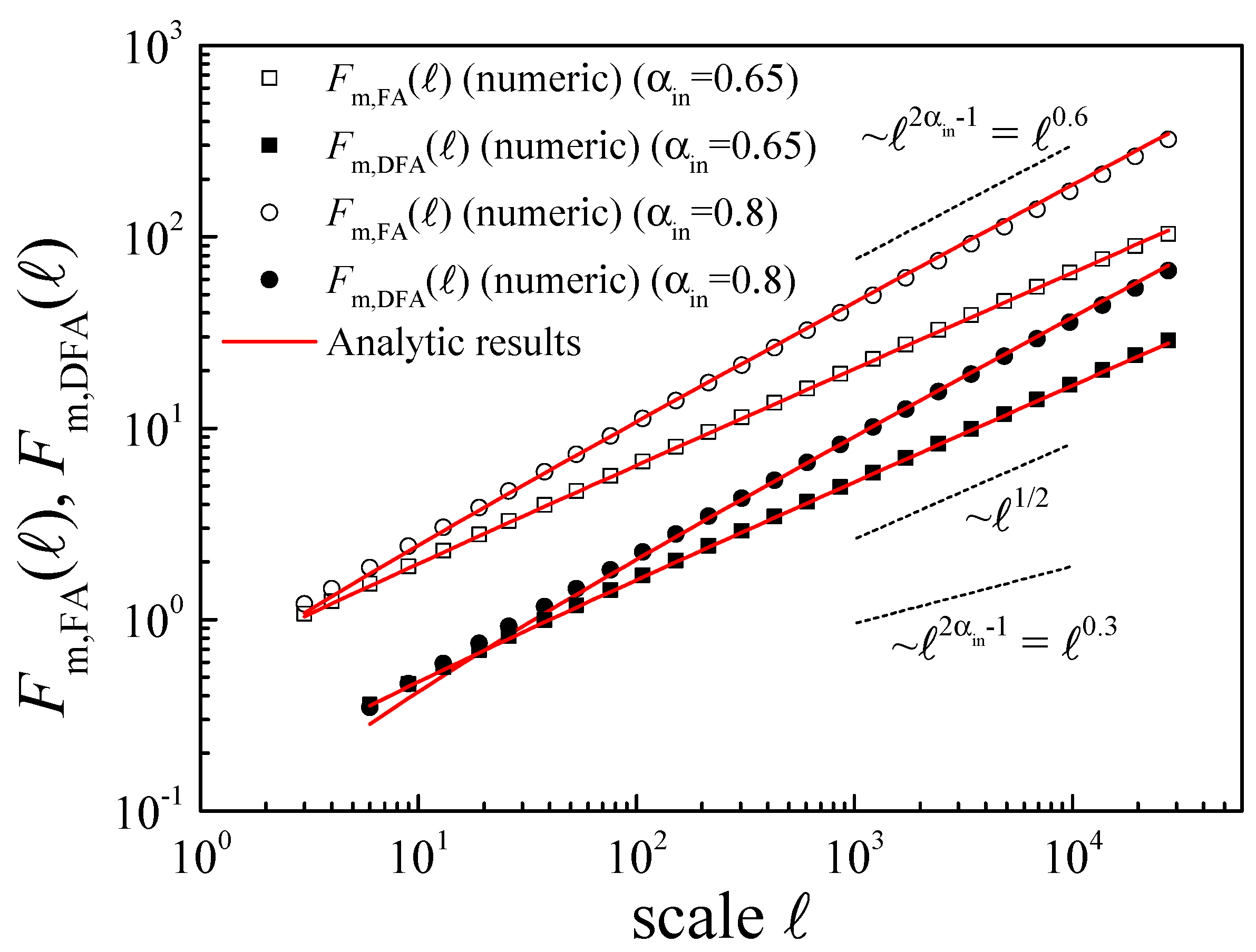
The validity of this analytic result is shown in Figure 6, where we plot obtained numerically in magnitude time series from fGns generated using FFM for two values of (open symbols), and also the corresponding analytical values using Equation (43), shown in solid lines. Equation (43) explains the results obtained using FA (21): for , i.e., , the second term in the sum dominates asymptotically and then leading to (see the case in Figure 6). In contrast, for , i.e., , the first term in the sum is the dominant one and from where , as the case in Figure 6.
A similar, though more elaborated calculation can be carried out for the scaling of the magnitude series using DFA. In this case, starting from Equation (11), we write for the magnitude series
where, as before, . Using Equation (30), we get:
To evaluate this equation, we insert the expression of (Equation (34)), use the definitions of (Equation (12)) and (Equation (13)), substitute the sum by a definite integral and calculate it, and simplify the results by keeping the highest powers of ℓ to get the (asymptotically correct) result:
The validity of this last equation is also shown in Figure 6, where we plot for two different values the numerical functions provided by DFA (solid symbols) and the corresponding analytic functions from Equation (46) (solid lines). Similarly to the FA case, Equation (46) allows for understanding the spurious results (21) obtained using DFA. As before, for , i.e., for (see the case in Figure 6), the second term in the sum dominates for large ℓ and then , or . For , i.e., (see the case in Figure 6), the first term in the sum is the dominant one and from where .
We conclude that the spurious FA and DFA result for is due to the existence of a first term proportional to ℓ in Equations (43) and (46), which dominates asymptotically when . The correct result for could only be obtained by FA and DFA without such ℓ-term in Equations (43) and (46), which, regrettably, is an intrinsic property of both techniques.
8. Conclusions
We have shown that the magnitude and sign series obtained from power-law correlated stationary time series, such as fractional Gaussian noises, are also power-law correlated for any scaling of the original series. Indeed, we have obtained analytical expressions for both power-law autocorrelation functions confirmed by numerical results. However, when the magnitude and sign series are analyzed using Fluctuation Analysis and Detrended Fluctuation Analysis, also known as the magnitude and sign decomposition method, depending on the scaling of the original time series, both techniques can provide spurious scaling results and lead to wrongly interpreting the magnitude and sign series as completely uncorrelated (white noises). By using the relationships between the autocorrelation functions and the fluctuation functions of FA and DFA, we find analytically and confirm numerically the reason for these spurious results, which turns out to be an intrinsic property of both methods.
Acknowledgments
We acknowledge the Spanish Junta de Andalucía for financial support (Grants FQM-362 and FQM-7964).
Author Contributions
Pedro Carpena conceived the research and carried out the analytical calculations; and all authors performed the numerical experiments and wrote the paper.
Conflicts of Interest
The authors declare no conflict of interest.
References
- Hurst, H.E. Long-term storage capacity of reservoirs. Trans. Am. Soc. Civ. Eng. 1951, 116, 770–799. [Google Scholar]
- Peng, C.K.; Buldyrev, S.V.; Goldberger, A.L.; Havlin, S.; Sciortino, F.; Simons, M.; Stanley, H.E. Long-range correlations in nucleotide sequences. Nature 1992, 356, 168–170. [Google Scholar] [CrossRef] [PubMed]
- Peng, C.K.; Buldyrev, S.V.; Havlin, S.; Simons, M.; Stanley, H.E.; Goldberger, A.L. Mosaic organization of DNA nucleotides. Phys. Rev. E 1994, 49, 1685–1689. [Google Scholar] [CrossRef]
- Ashkenazy, Y.; Ivanov, P.C.; Havlin, S.; Peng, C.K.; Goldberger, A.L.; Stanley, H.E. Magnitude and Sign Correlations in Heartbeat Fluctuations. Phys. Rev. Lett. 2001, 86, 1900–1903. [Google Scholar] [CrossRef] [PubMed]
- Gomez-Extremera, M.; Carpena, P.; Ivanov, P.C.; Bernaola-Galván, P.A. Magnitude and sign of long-range correlated time series: Decomposition and surrogate signal generation. Phys. Rev. E 2016, 93, 042201. [Google Scholar] [CrossRef] [PubMed]
- Ashkenazy, Y.; Havlin, S.; Ivanov, P.C.; Peng, C.K.; Schulte-Frohlinde, V.; Stanley, H.E. Magnitude and sign scaling in power-law correlated time series. Physica A 2003, 323, 19–41. [Google Scholar] [CrossRef]
- Kalisky, T.; Ashkenazy, Y.; Havlin, S. Volatility of linear and nonlinear time series. Phys. Rev. E 2005, 72, 011913. [Google Scholar] [CrossRef] [PubMed]
- Kantelhardt, J.W.; Ashkenazy, Y.; Ivanov, P.C.; Bunde, A.; Havlin, S.; Penzel, T.; Peter, J.H.; Stanley, H.E. Characterization of sleep stages by correlations in the magnitude and sign of heartbeat increments. Phys. Rev. E 2002, 65, 051908. [Google Scholar] [CrossRef] [PubMed]
- Bernaola-Galván, P.A.; Gómez-Extremera, M.; Romance, A.R.; Carpena, P. Correlations in magnitude series to assess nonlinearities: Application to multifractal models and heartbeat fluctuations. arXiv 2017. [Google Scholar]
- Zhu, L.; Jin, N.D.; Gao, Z.K.; Zong, Y.B.; Zhai, L.S.; Wang, Z.Y. Magnitude and sign correlations in conductance fluctuations of horizontal oil water two-phase flow. J. Phys. Conf. Ser. 2012, 364, 012067. [Google Scholar] [CrossRef]
- Makse, H.A.; Davies, G.W.; Havlin, S.; Ivanov, P.C.; King, P.R.; Stanley, H.E. Long-range correlations in permeability fluctuations in porous rock. Phys. Rev. E 1996, 54, 3129–3134. [Google Scholar] [CrossRef]
- Makse, H.A.; Havlin, S.; Ivanov, P.C.; King, P.R.; Prakash, S.; Stanley, H.E. Pattern formation in sedimentary rocks: Connectivity, permeability, and spatial correlations. Physica A 1996, 233, 587–605. [Google Scholar] [CrossRef]
- Bartos, I.; Jánosi, I.M. Nonlinear correlations of daily temperature records over land. Nonlinear Process. Geophys. 2006, 13, 571–576. [Google Scholar] [CrossRef]
- Li, Q.; Fu, Z.; Yuan, N.; Xie, F. Effects of non-stationarity on the magnitude and sign scaling in the multi-scale vertical velocity increment. Physica A 2014, 410, 9–16. [Google Scholar] [CrossRef]
- Liu, Y.; Gopikrishnan, P.; Cizeau, P.; Meyer, M.; Peng, C.K.; Stanley, H.E. Statistical properties of the volatility of price fluctuations. Phys. Rev. E 1999, 60, 1390–1400. [Google Scholar] [CrossRef]
- Beran, J. Statistics for Long-Memory Processes; Chapman and Hall/CRC: Boca Raton, FL, USA, 1994. [Google Scholar]
- Coronado, A.V.; Carpena, P. Size effects on correlation measures. J. Biol. Phys. 2005, 31, 121–133. [Google Scholar] [CrossRef] [PubMed]
- Bryce, R.M.; Sprague, K.B. Revisiting detrended fluctuation analysis. Sci. Rep. 2012, 2, 315. [Google Scholar] [CrossRef] [PubMed]
- Allegrini, P.; Barbi, M.; Grigolini, P.; West, B.J. Dynamical model for DNA sequences. Phys. Rev. E 1995, 52, 5281–5296. [Google Scholar] [CrossRef]
- Molchan, G.M. Maximum of fractional Brownian motion: Probabilities of small values. Commun. Math. Phys. 1999, 205, 97–111. [Google Scholar] [CrossRef]
- Rangarajan, G.; Ding, M.Z. Integrated approach to the assessment of long range correlation in time series data. Phys. Rev. E 2000, 61, 4991–5001. [Google Scholar] [CrossRef]
- Hu, K.; Ivanov, P.C.; Chen, Z.; Carpena, P.; Stanley, H.E. Effect of trends on detrended fluctuation analysis. Phys. Rev. E 2001, 64, 011114. [Google Scholar] [CrossRef] [PubMed]
- Chen, Z.; Hu, K.; Carpena, P.; Bernaola-Galván, P.; Stanley, H.E.; Ivanov, P.C. Effect of nonlinear filters on detrended fluctuation analysis. Phys. Rev. E 2005, 71, 011104. [Google Scholar] [CrossRef] [PubMed]
- Blázquez, M.T.; Anguiano, M.; de Saavedra, F.A.; Lallena, A.M.; Carpena, P. Study of the human postural control system during quiet standing using detrended fluctuation analysis. Phys. A 2009, 388, 1857–1866. [Google Scholar] [CrossRef]
- Carpena, P.; Bernaola-Galván, P.; Coronado, A.V.; Hackenberg, M.; Oliver, J.L. Identifying characteristic scales in the human genome. Phys. Rev. E 2007, 75, 032903. [Google Scholar] [CrossRef] [PubMed]
- Karlin, S.; Brendel, V. Patchiness and correlations in DNA sequences. Science 1993, 259, 677–680. [Google Scholar] [CrossRef] [PubMed]
- Höll, M.; Kantz, H. The relationship between the detrended fluctuation analysis and the autocorrelation function of a signal. Eur. Phys. J. B 2015, 88, 327. [Google Scholar] [CrossRef]
- Talkner, P.; Weber, R.O. Power spectrum and detrended fluctuation analysis: Application to daily temperatures. Phys. Rev. E 2000, 62, 150–160. [Google Scholar] [CrossRef]
- Carretero-Campos, C.; Bernaola-Galván, P.; Ivanov, P.C.; Carpena, P. Phase transitions in the first-passage time of scale-invariant correlated processes. Phys. Rev. E 2012, 85, 011139. [Google Scholar] [CrossRef] [PubMed]
- Makse, H.A.; Havlin, S.; Schwartz, M.; Stanley, H.E. Method for generating long-range correlations for large systems. Phys. Rev. E 1996, 53, 5445–5449. [Google Scholar] [CrossRef]
- Bernaola-Galván, P.; Oliver, J.L.; Hackenberg, M.; Coronado, A.V.; Ivanov, P.C.; Carpena, P. Segmentation of time series with long-range fractal correlations. Eur. Phys. J. B 2012, 85, 211. [Google Scholar] [CrossRef] [PubMed]
- Apostolov, S.S.; Izrailev, F.M.; Makarov, N.M.; Mayzelis, Z.A.; Melnyk, S.S.; Usatenko, O.V. The Signum function method for the generation of correlated dichotomic chains. J. Phys. A Math. Theor. 2008, 41, 175101. [Google Scholar] [CrossRef]
Figure 1.
(a) a fractional Gaussian noise-type time series, , generated using the Fourier Filtering Method (FFM) with and ; (b) the sign series obtained from ; and (c) the magnitude (or volatility) series obtained from .
Figure 1.
(a) a fractional Gaussian noise-type time series, , generated using the Fourier Filtering Method (FFM) with and ; (b) the sign series obtained from ; and (c) the magnitude (or volatility) series obtained from .
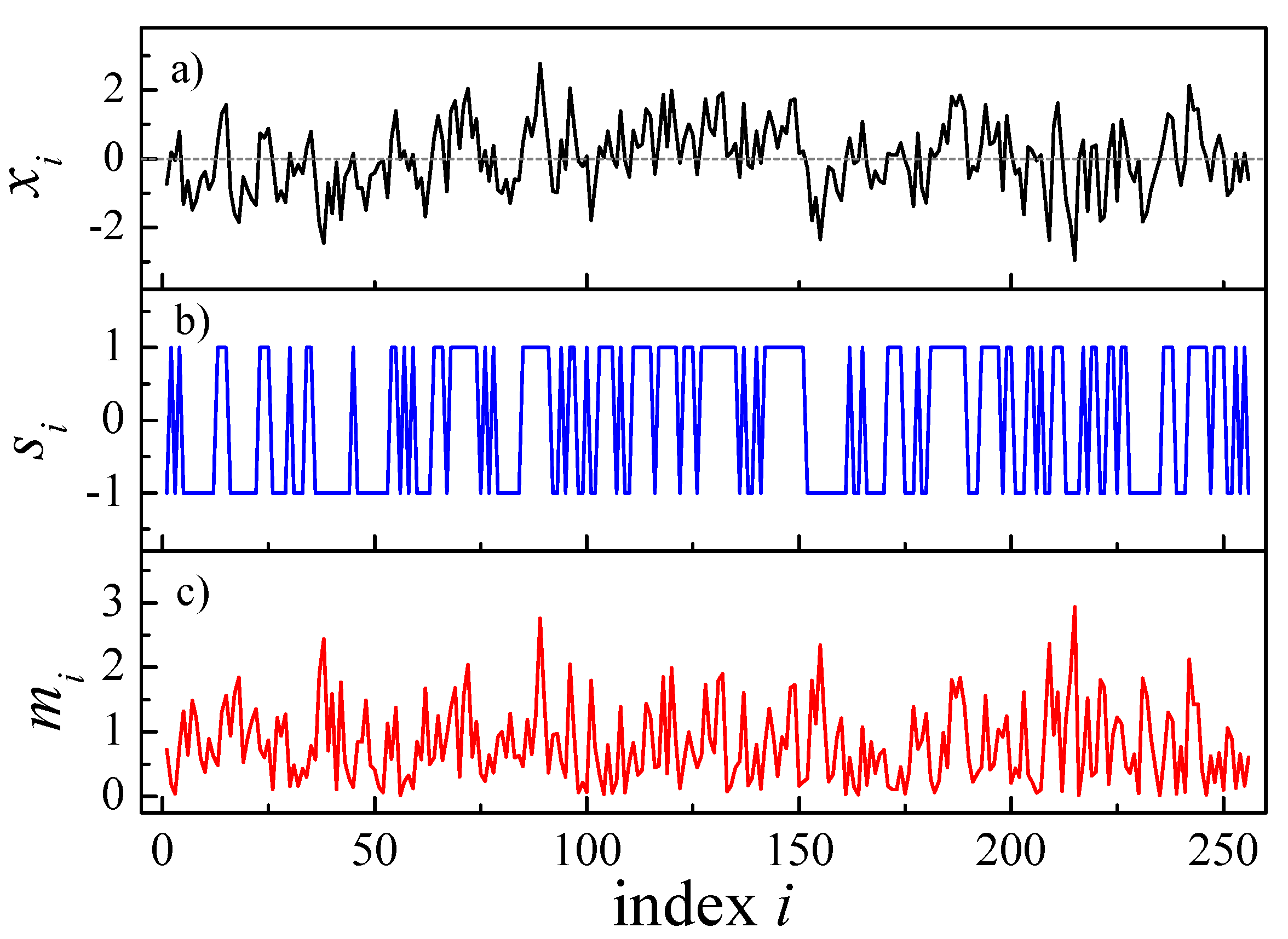
Figure 2.
The sign scaling exponent and the magnitude scaling exponent as a function of the scaling exponent of the original signal. Top panel: results of Fluctuation Analysis (FA); bottom panel: results of Detrended Fluctuation Analysis (DFA). We have used time series with , and we have generated 200 series for any value.

Figure 3.
The sign (a) and magnitude (b) autocorrelation functions, and , as a function of the values of the autocorrelation function of the original time series, . The solid lines correspond to the exact analytical results (Equations (27) and (28)), and the dashed lines to the first term in the corresponding Taylor expansions (Equations (29) and (30)).
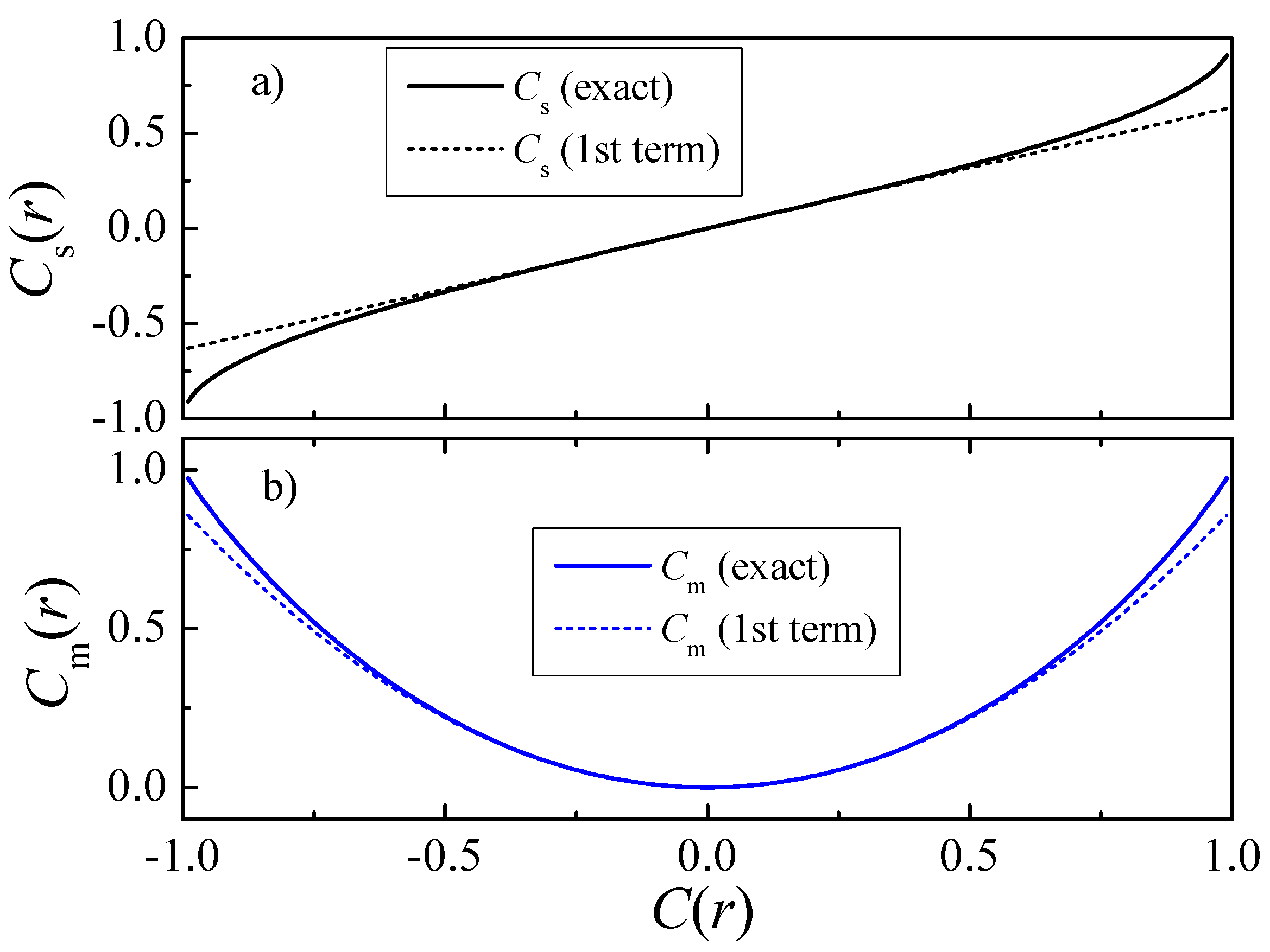
Figure 4.
Autocorrelation function of the original time series (), of the sign series () and of the magnitude series () obtained numerically for synthetic fractional Gaussian noises (fGns) generated with different values. (a–d) correspond to situations where the original fGn presents positive correlations (); (e,f) show examples in which the fGn is anticorrelated (). As, in this case, both and are negative, (e,f) show the absolute value of and . In all cases, the lines correspond to the analytical values of (solid lines) and (dotted lines) obtained from using Equations (29) and (30). For any value, we generate 100 fGns of length and average the corresponding , and .
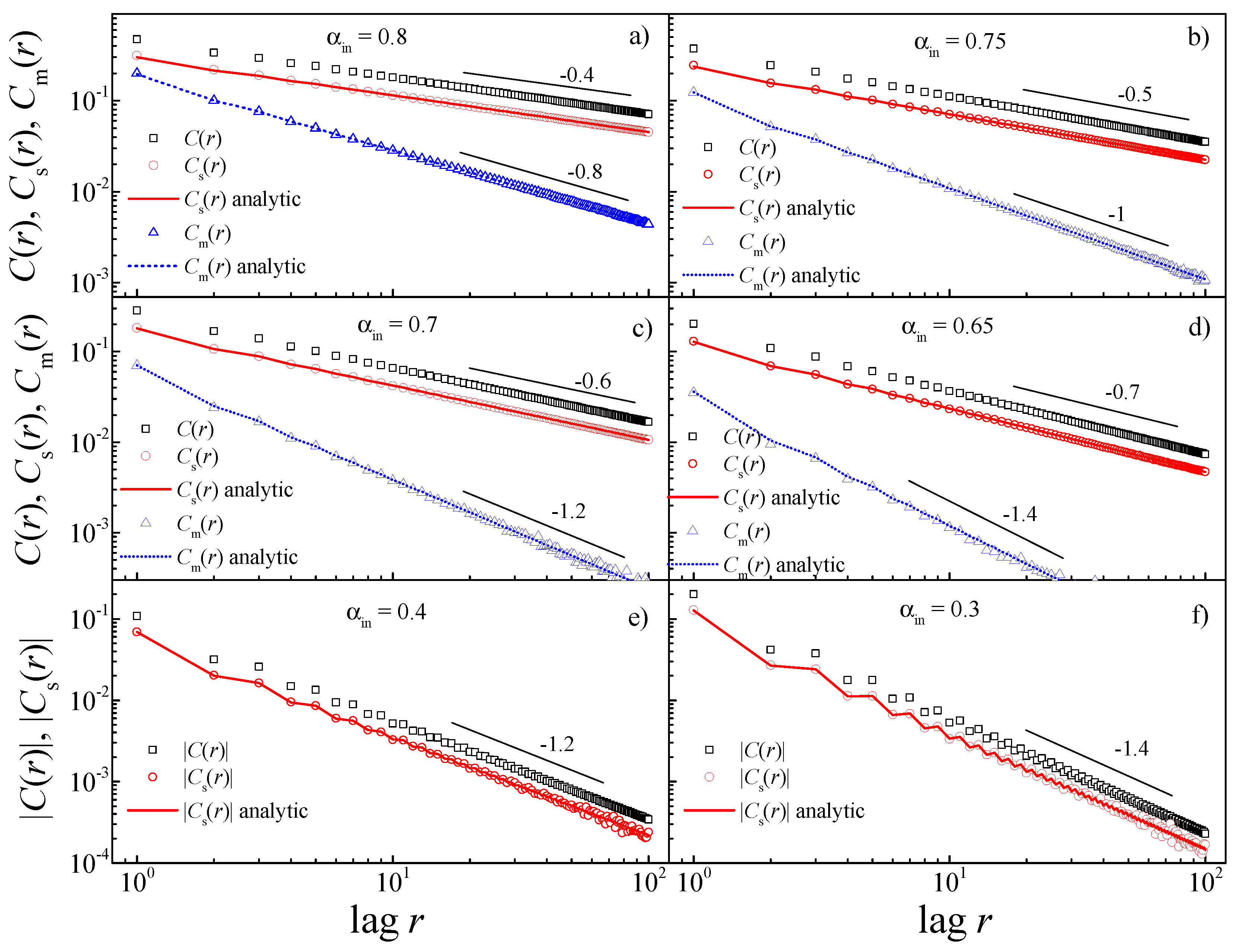
Figure 5.
Magnitude and sign scaling exponents, and provided by FA and DFA (symbols), and the correct results for and (lines) expected from the corresponding autocorrelation functions.
Figure 5.
Magnitude and sign scaling exponents, and provided by FA and DFA (symbols), and the correct results for and (lines) expected from the corresponding autocorrelation functions.

Figure 6.
FA and DFA Fluctuation functions for the magnitude series obtained from two fGns with and , and . The numeric results of applying FA and DFA to the corresponding time series are shown in symbols, and the lines correspond to the analytical results obtained from Equations (43) and (46). We also include dashed lines corresponding to the correct scaling , which gives and for and , respectively, and to the spurious scaling . Note how FA and DFA predict the correct scaling exponent for but fail for since, instead of , both techniques give .
© 2017 by the authors. Licensee MDPI, Basel, Switzerland. This article is an open access article distributed under the terms and conditions of the Creative Commons Attribution (CC BY) license (http://creativecommons.org/licenses/by/4.0/).
Share and Cite
MDPI and ACS Style
Carpena, P.; Gómez-Extremera, M.; Carretero-Campos, C.; Bernaola-Galván, P.; Coronado, A.V. Spurious Results of Fluctuation Analysis Techniques in Magnitude and Sign Correlations. Entropy 2017, 19, 261. https://doi.org/10.3390/e19060261
AMA Style
Carpena P, Gómez-Extremera M, Carretero-Campos C, Bernaola-Galván P, Coronado AV. Spurious Results of Fluctuation Analysis Techniques in Magnitude and Sign Correlations. Entropy. 2017; 19(6):261. https://doi.org/10.3390/e19060261
Chicago/Turabian StyleCarpena, Pedro, Manuel Gómez-Extremera, Concepción Carretero-Campos, Pedro Bernaola-Galván, and Ana V. Coronado. 2017. "Spurious Results of Fluctuation Analysis Techniques in Magnitude and Sign Correlations" Entropy 19, no. 6: 261. https://doi.org/10.3390/e19060261
Note that from the first issue of 2016, this journal uses article numbers instead of page numbers. See further details here.