
The Entropy of Words—Learnability and Expressivity across More than 1000 Languages


Abstract
:
1. Introduction
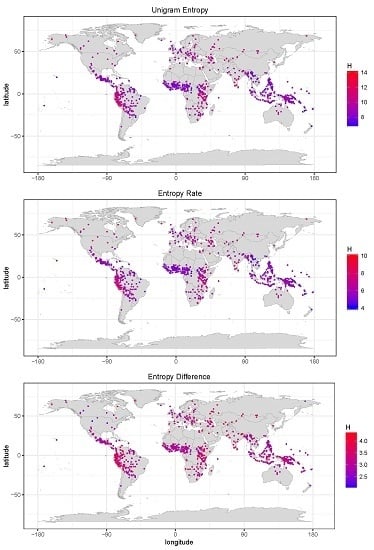
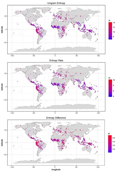
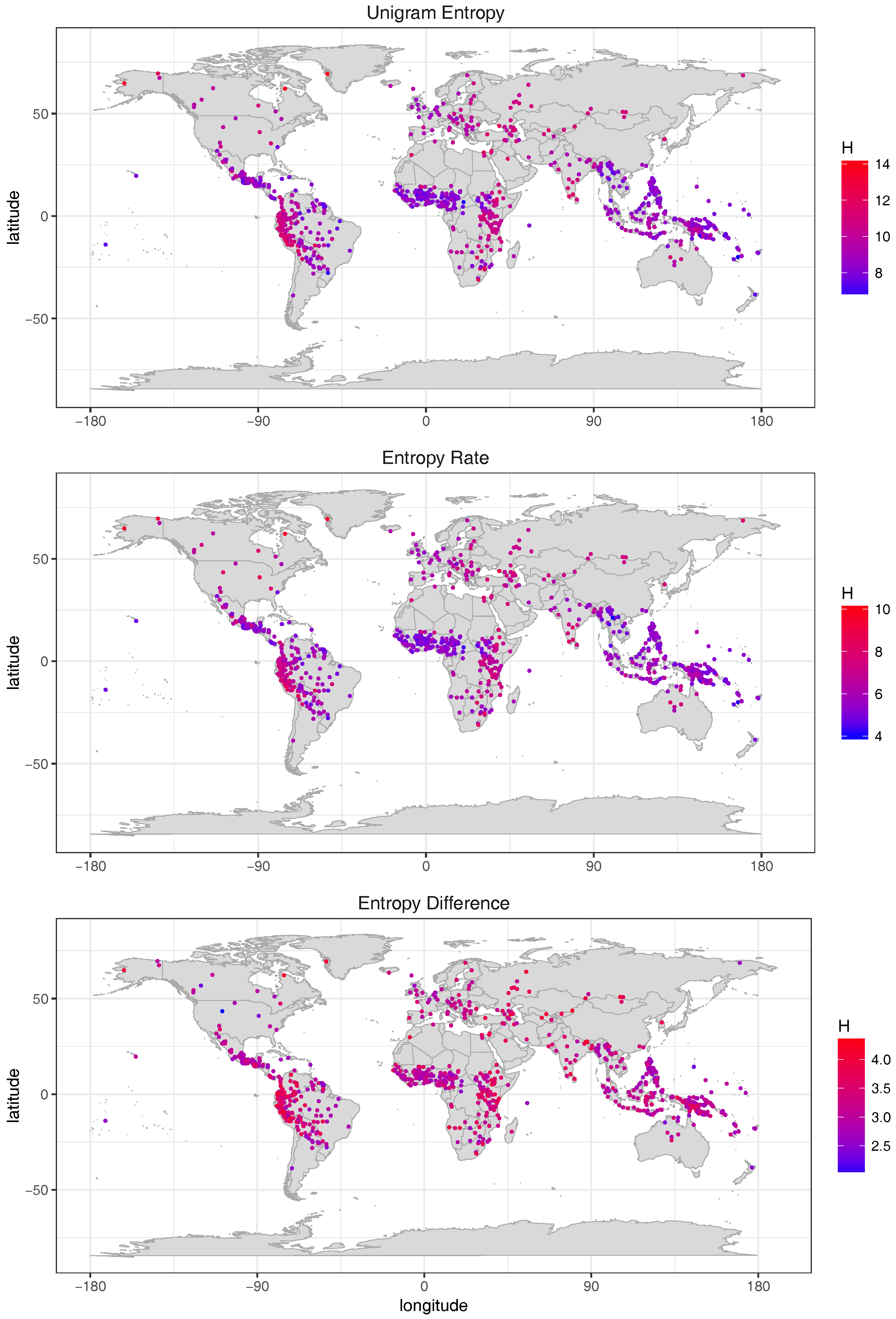
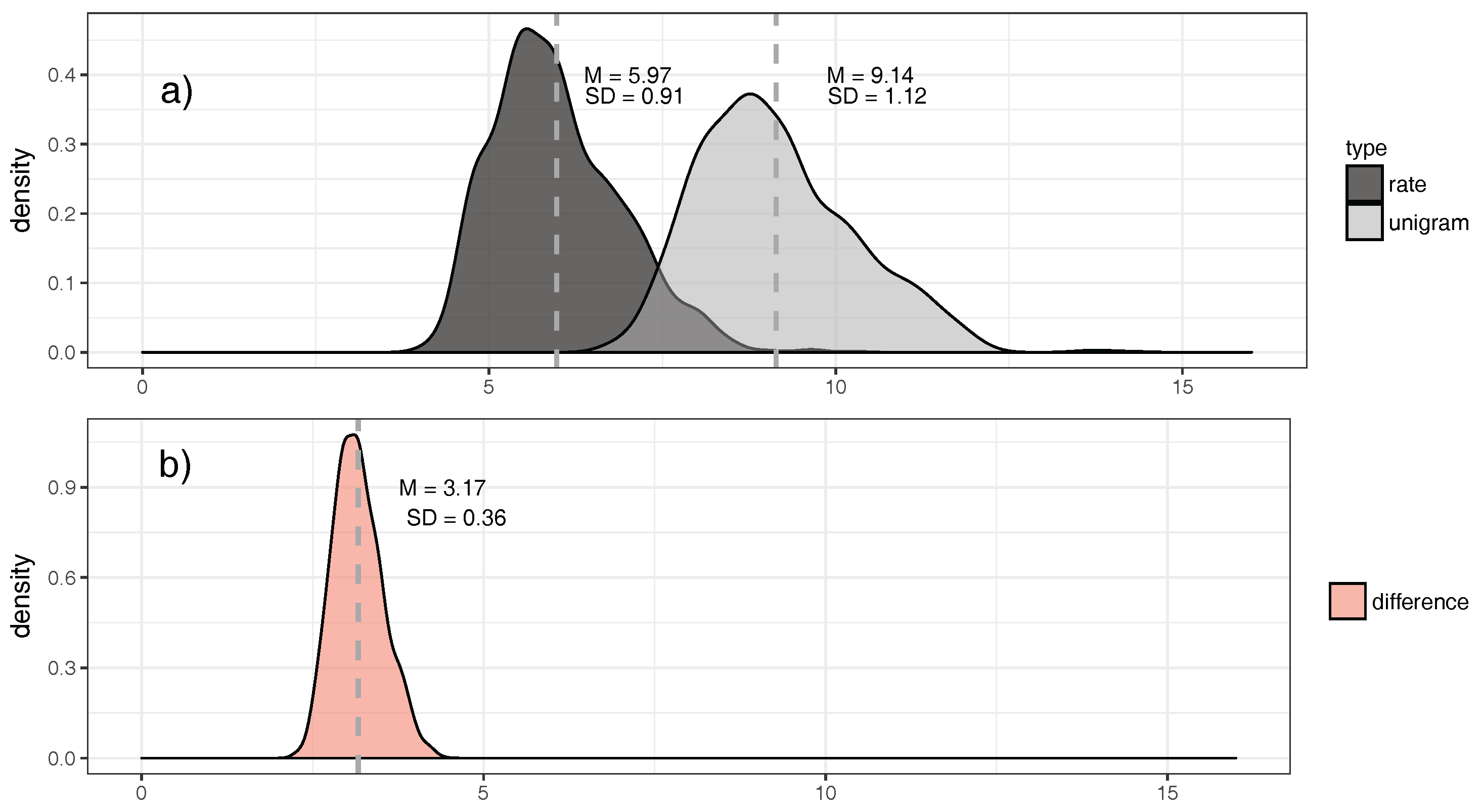
- Across languages of the world, unigram entropies display a unimodal distribution around a mean of ca. nine bits/word, with a standard deviation of ca. one bit/word. Entropy rates have a lower mean of ca. six bits/word, with a standard deviation of ca. one bit/word. Hence, there seem to be strong pressures keeping the mass of languages in a relatively narrow entropy range. This is particularly salient for the difference between unigram entropy and entropy rate (Section 5.2).
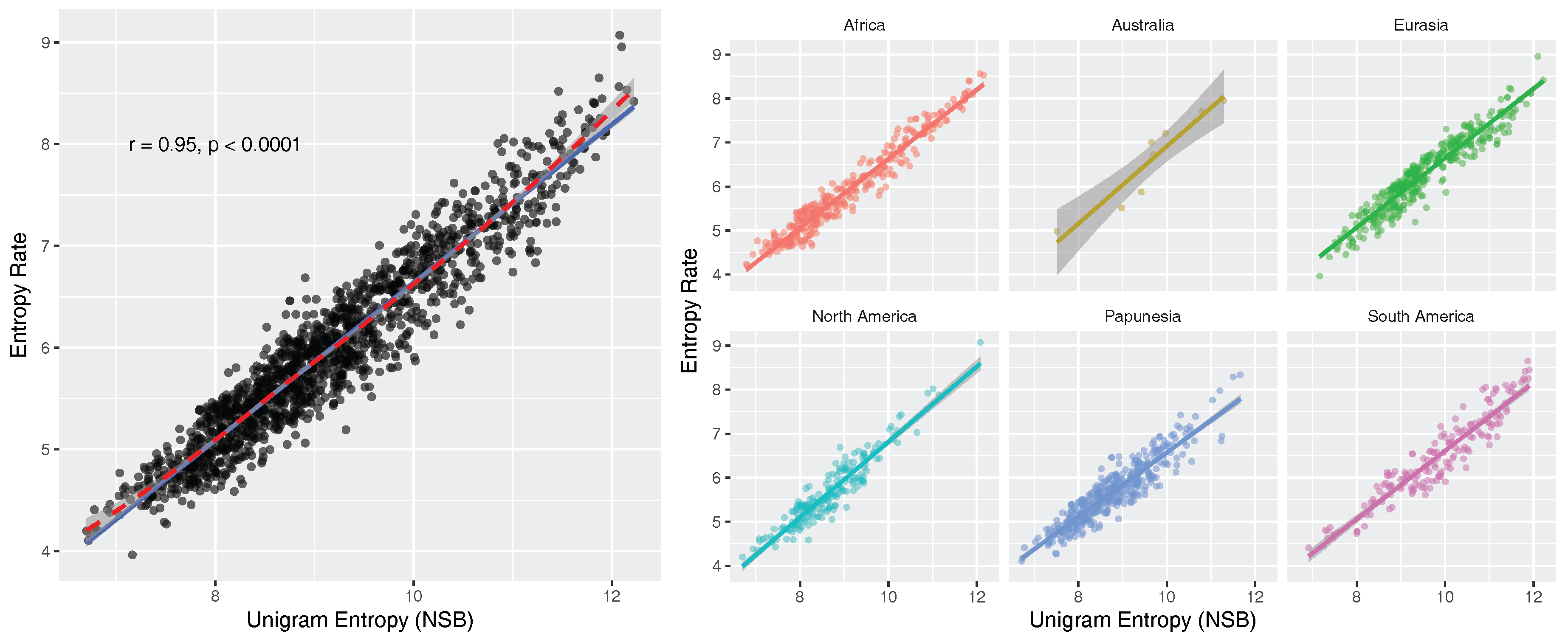
- There is a strong positive linear relationship between unigram entropies and entropy rates (). To our knowledge, this has not been reported before. We formulate a simple linear model that predicts the entropy rate of a text from the unigram entropy of the same text: , where and (Section 5.3). The implication of this relationship is that uncertainty-reduction by co-textual information is approximately linear across languages of the world.
2. Data
3. Theory
3.1. Word Types and Tokens
The set of word types (in lower case) for this sentence is:in the beginning god created the heavens and the earth and the earth was waste and empty [...]
3.2. Entropy Estimation
3.2.1. General Conditions
3.2.2. Word Entropy Estimation
in the beginning god created the heavens and the earth and the earth was waste and empty [...]
3.2.3. Problem 1: The Infinite Productive Potential of Languages
3.2.4. Problem 2: Short- and Long-Range Correlations between Words
3.2.5. Our Perspective
3.2.6. n-Gram Entropies
3.2.7. Entropy Rate
in1 the2 beginning3 god4 created5 the6 heavens7 and8 the9 earth10 and11 the12 earth13 was14 waste15 and16 empty17 [...]
4. Methods
4.1. Entropy Estimation Software
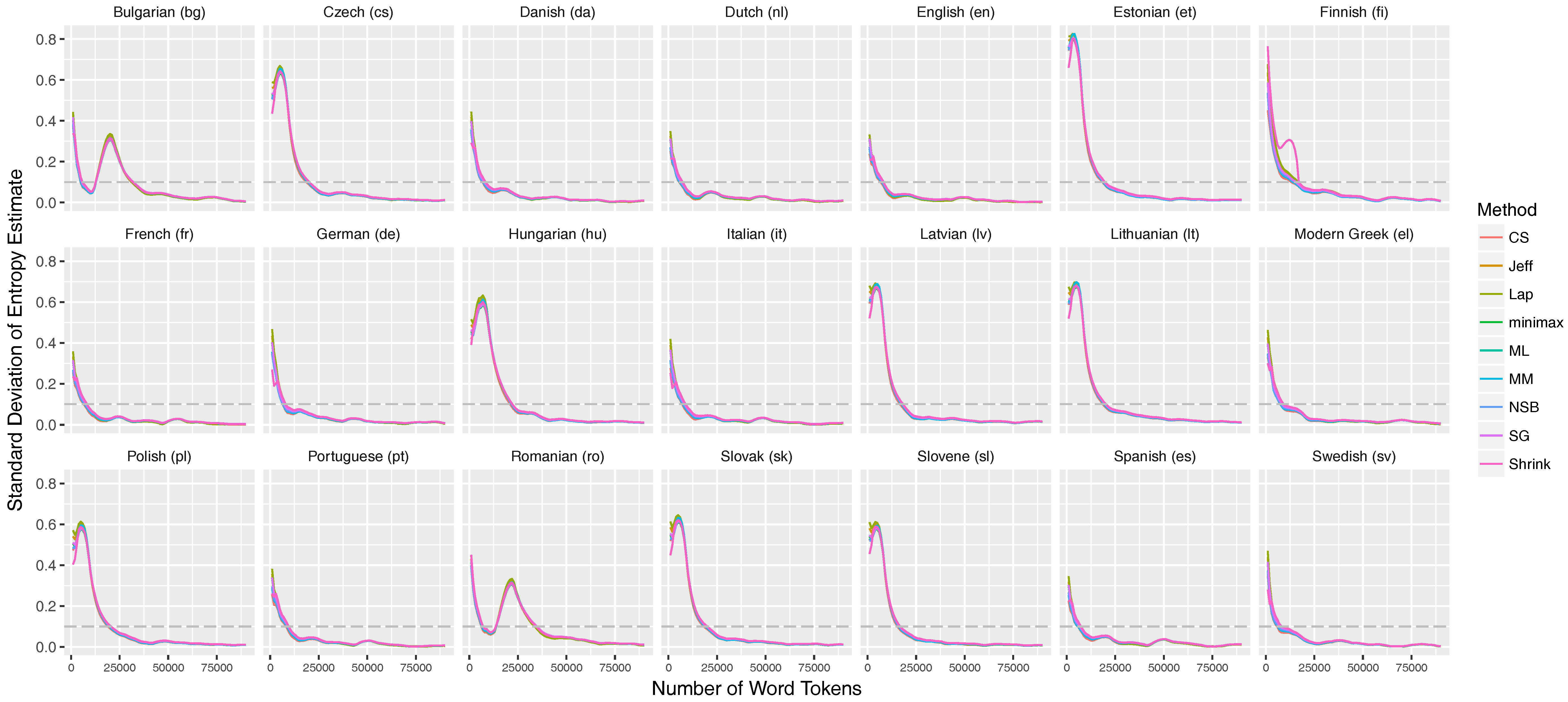
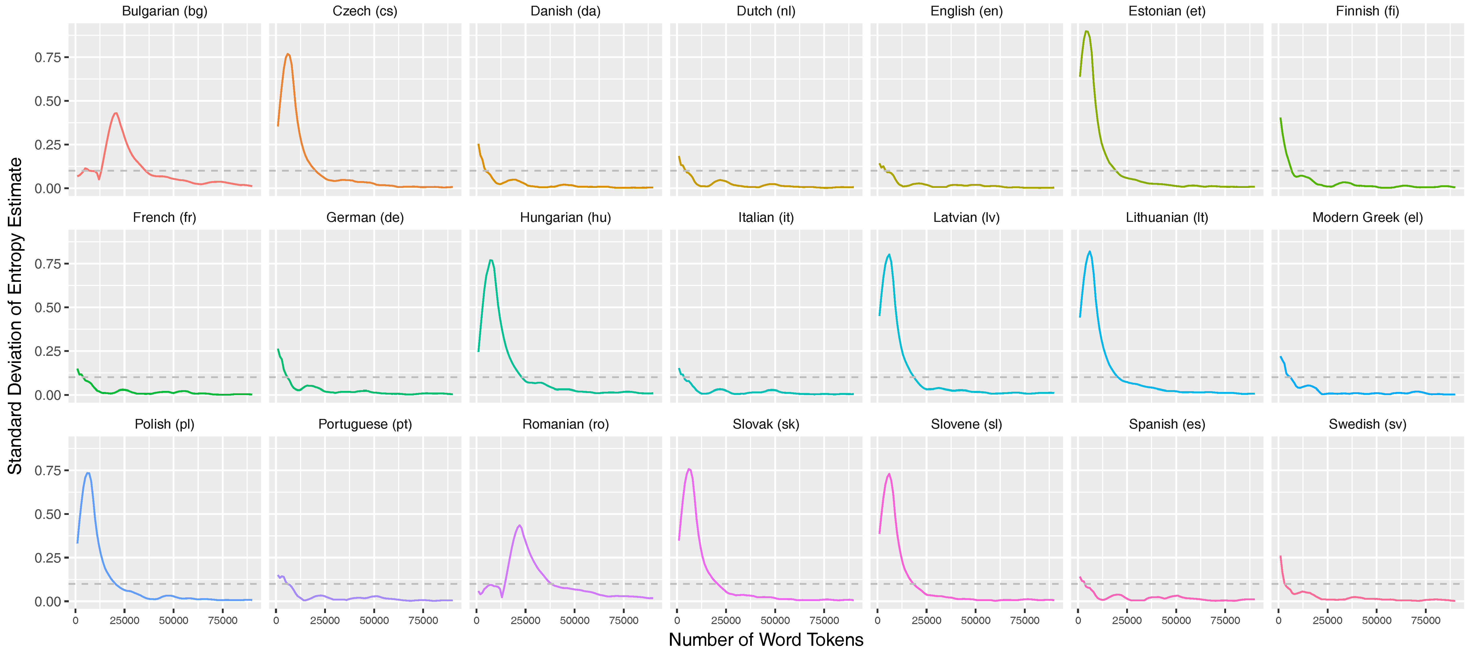
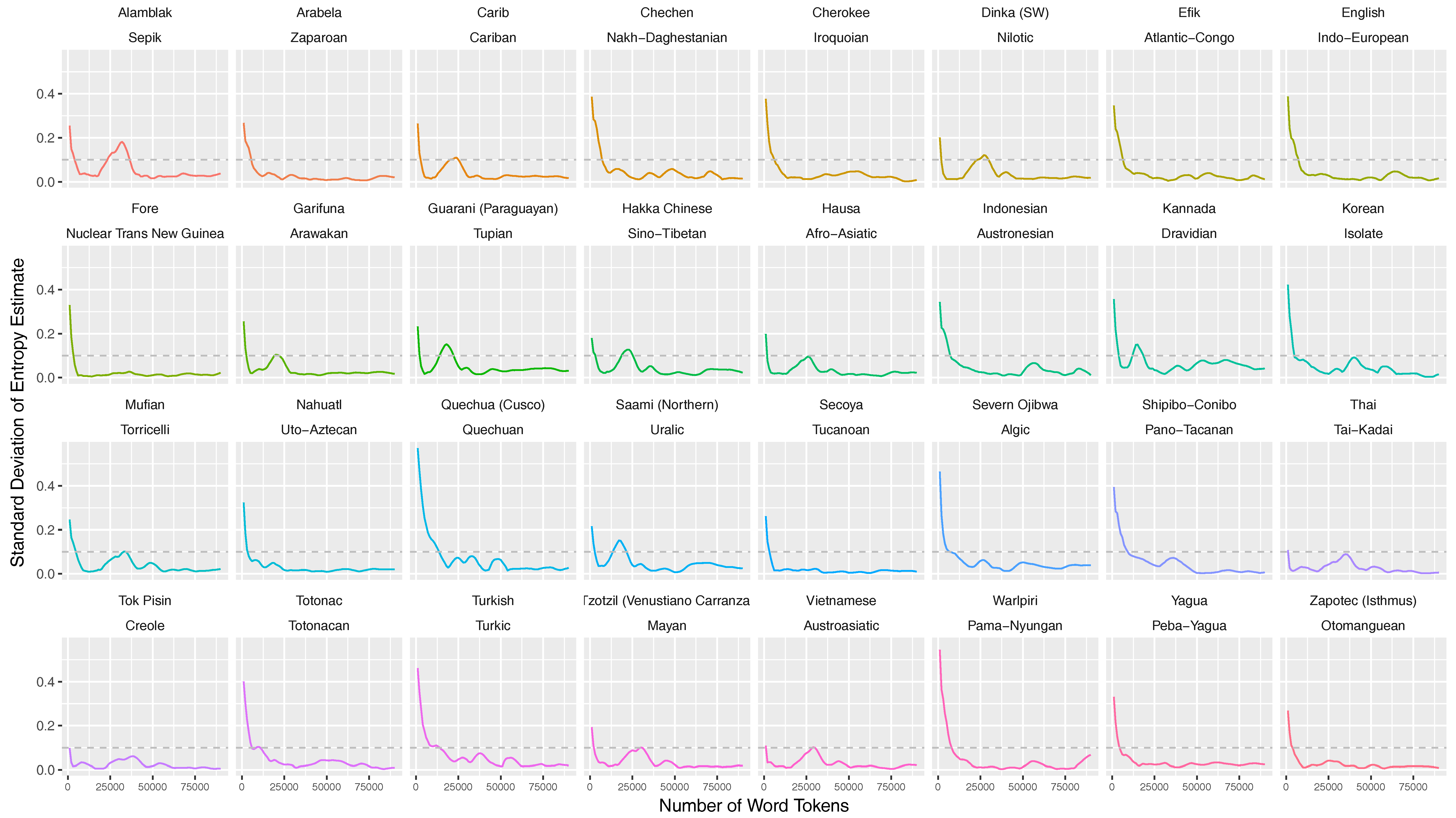
4.2. Stabilization Criterion
4.3. Corpus Samples
5. Results
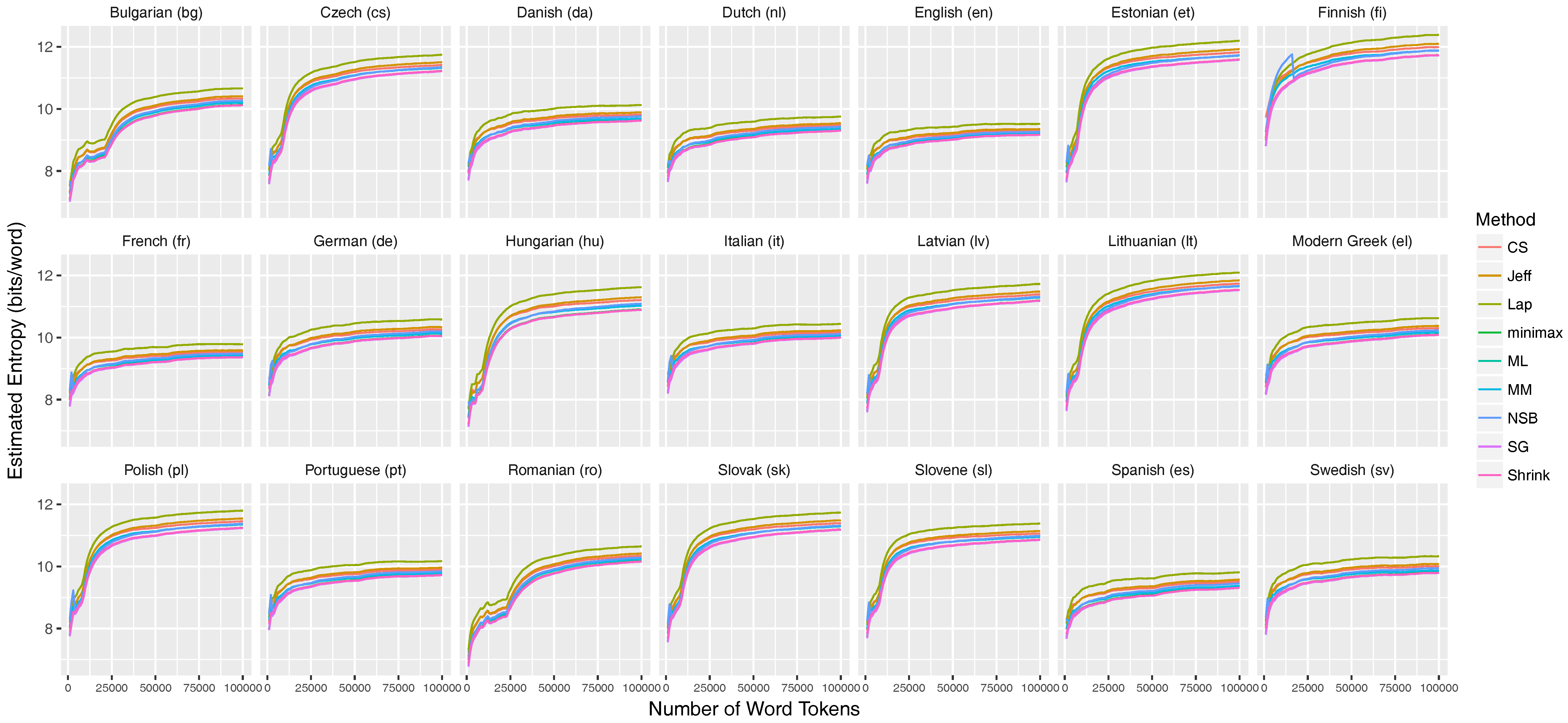
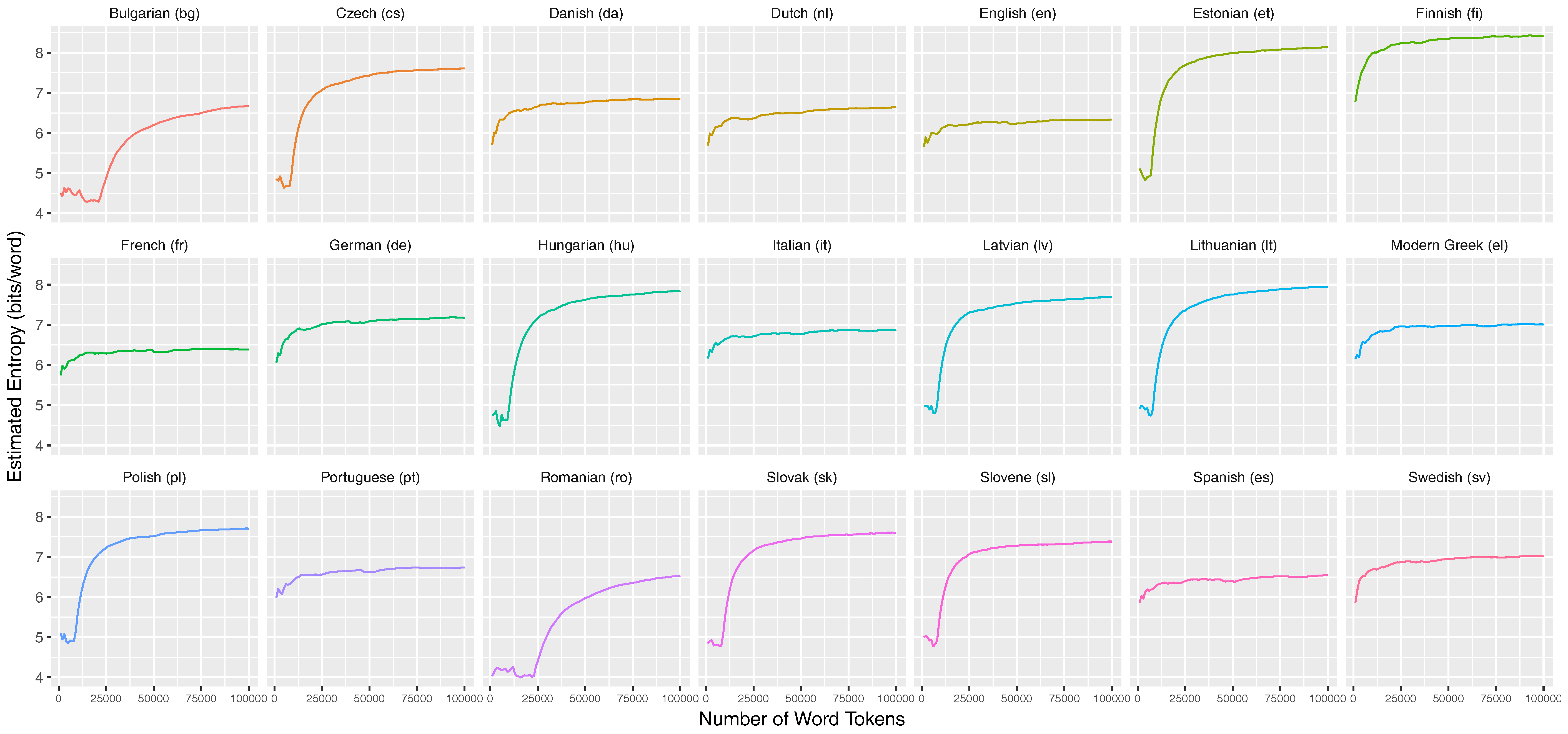
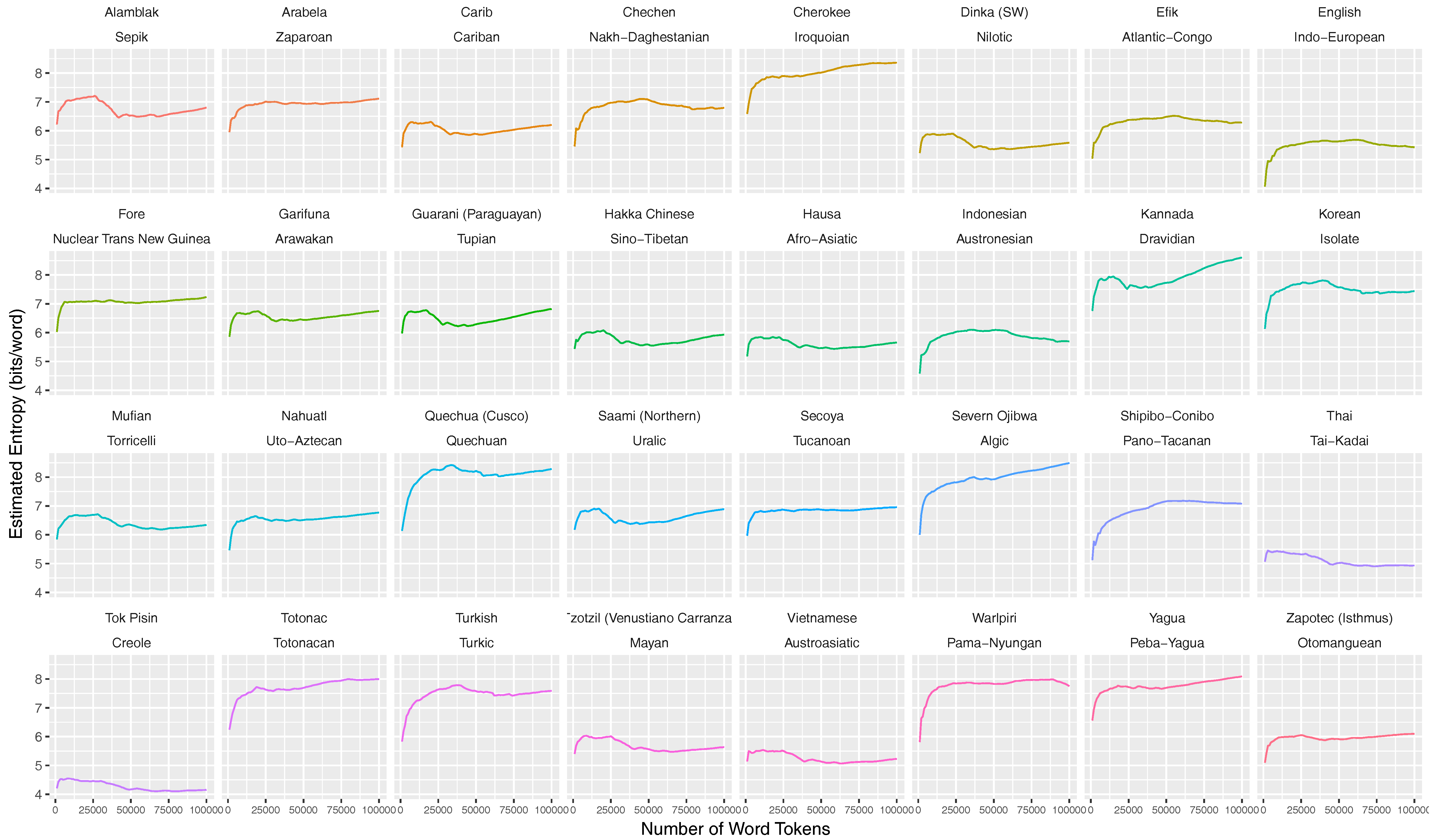
5.1. Entropy Stabilization throughout the Text Sequence
5.2. Word Entropies across More than 1000 Languages
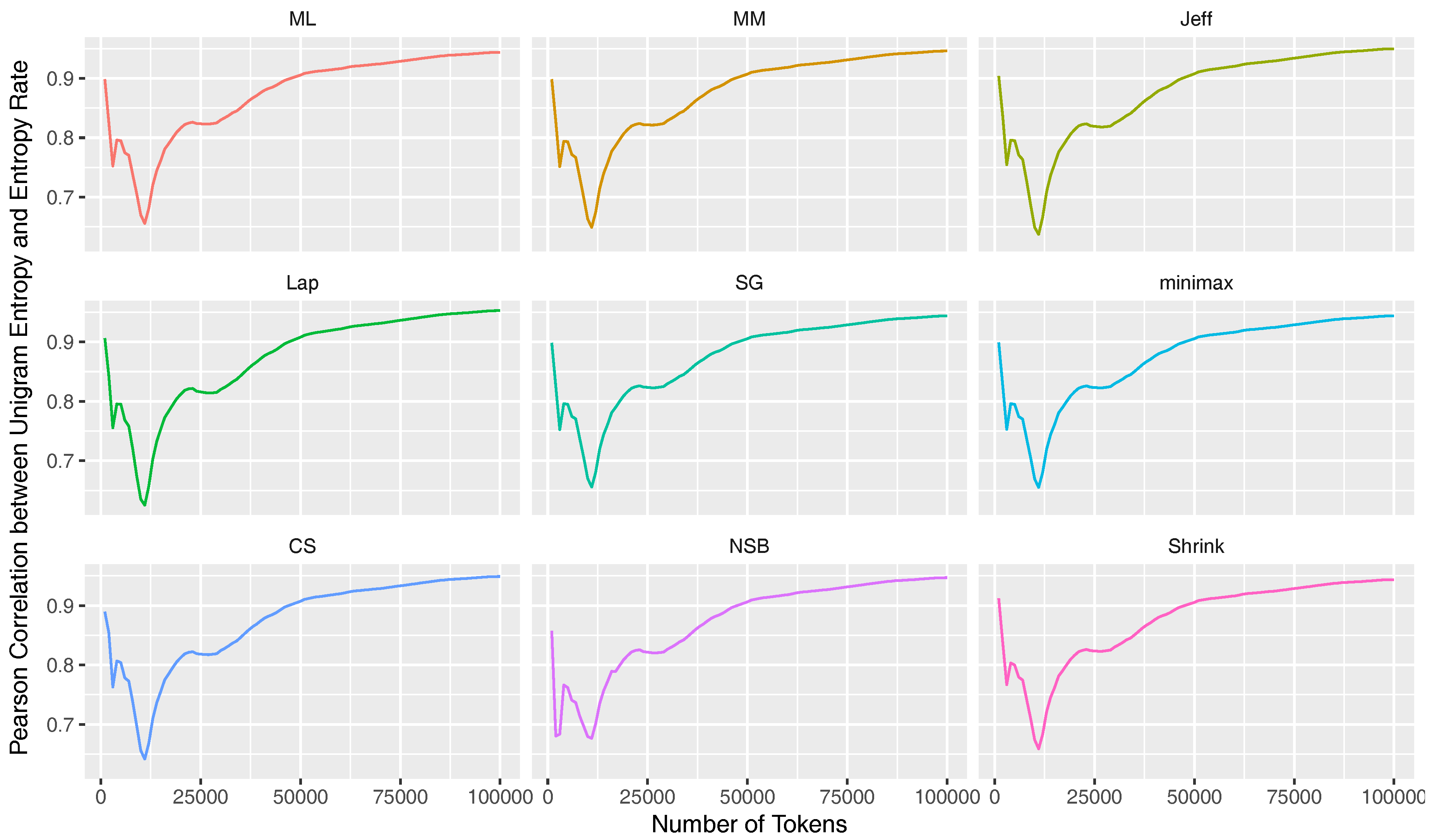
5.3. Correlation between Unigram Entropy and Entropy Rate
6. Discussion
6.1. Entropy Diversity across Languages of the World
6.2. Correlation between Unigram Entropies and Entropy Rates
7. Conclusions
Acknowledgments
Author Contributions
Conflicts of Interest
Abbreviations
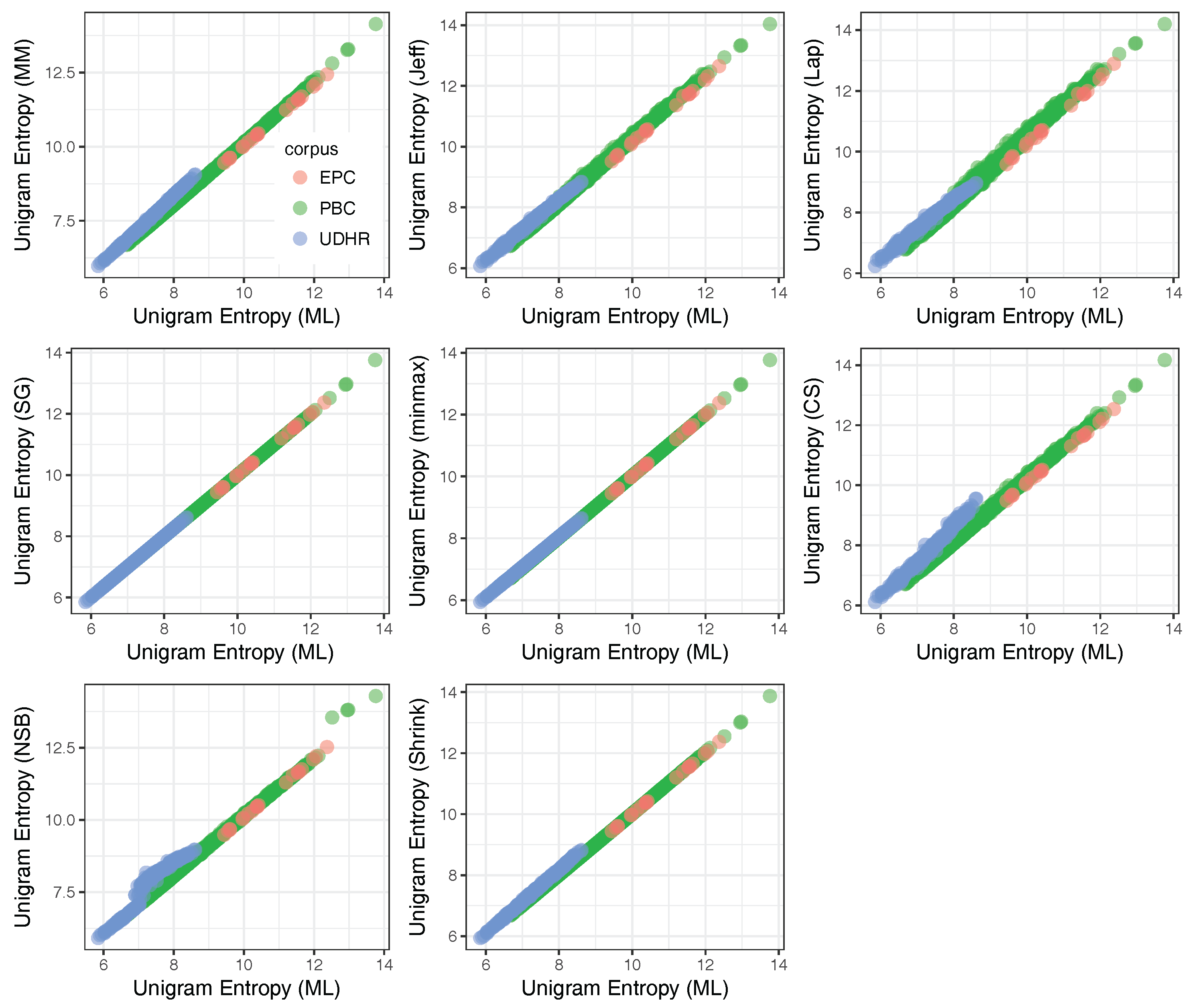
| EPC | European Parliament Corpus |
| PBC | Parallel Bible Corpus |
| UDHR | Universal Declaration of Human Rights |
| NSB | Nemenman–Shafee–Bialek |
Appendix A. Text Pre-Processing
Appendix A.1. Converting Letters to Lower Case
Appendix A.2. Removal of Punctuation
Although, as you will have seen, the dreaded “millennium bug” failed to materialise, [...]EPC (English, line 3)
And God said, let there be light . And there was light . [...]PBC (English, Genesis 1:3)
Furthermore, no distinction shall be made on the basis of the political, jurisdictional or international status of the country [...]UDHR (English, paragraph 3)
- For the EPC, we use the regular expression \\W+ in combination with the R function strsplit() to split strings of UTF-8 characters on punctuation and white spaces.
- For the PBC and UDHR, we define a regular expression meaning “at least one alpha-numeric character between white spaces” which would be written as: .*[[:alpha:]].*This regex can then be matched with the respective text to yield word types. This is done via the functions regexpr() and regmatches() in R.
Appendix B. Advanced Entropy Estimators
Appendix B.1. The Miller–Madow Estimator
Appendix B.2. Bayesian Estimators
Appendix B.3. The Chao–Shen Estimator
Appendix B.4. The James–Stein Shrinkage Estimator
Appendix C. Stabilization of the Entropy Rates for 21 Languages of the European Parliament Corpus
Appendix C.1. Unigram Entropies
Appendix C.2. Entropy Rate


Appendix D. Stabilization of Entropy Rates for 32 Languages of the Parallel Bible Corpus


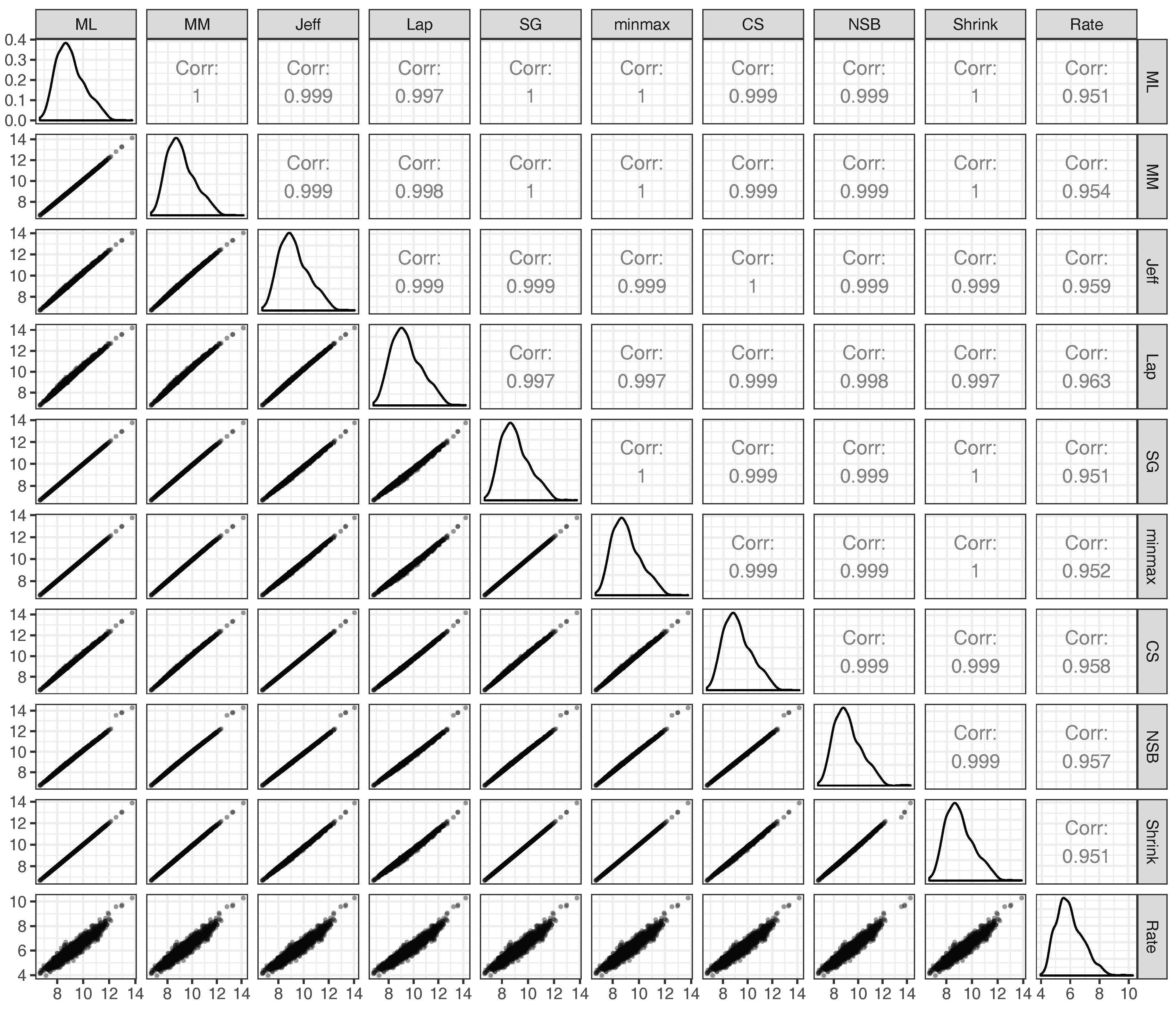
Appendix E. Correlations between Estimated Unigram Entropies


| - | ML | MM | Jeff | Lap | SG | minmax | CS | NSB | Shrink |
|---|---|---|---|---|---|---|---|---|---|
| ML | - | ||||||||
| MM | 0.9999405 | - | |||||||
| Jeff | 0.9994266 | 0.9996888 | - | ||||||
| Lap | 0.9983479 | 0.998819 | 0.9997185 | - | |||||
| SG | 1 | 0.9999405 | 0.9994267 | 0.998348 | - | ||||
| minmax | 0.9999999 | 0.9999445 | 0.9994415 | 0.9983733 | 0.9999999 | - | |||
| CS | 0.9993888 | 0.9996607 | 0.9999867 | 0.9997199 | 0.9993889 | 0.9994037 | - | ||
| NSB | 0.9997953 | 0.9999065 | 0.9998969 | 0.9992965 | 0.9997954 | 0.9998041 | 0.9998719 | - | |
| Shrink | 0.9999945 | 0.9999059 | 0.9993348 | 0.9981998 | 0.9999945 | 0.9999935 | 0.9992906 | 0.9997419 | - |
| - | ML | MM | Jeff | Lap | SG | minmax | CS | NSB | Shrink |
|---|---|---|---|---|---|---|---|---|---|
| ML | - | ||||||||
| MM | 0.9998609 | - | |||||||
| Jeff | 0.9989818 | 0.9993252 | - | ||||||
| Lap | 0.9969406 | 0.9975655 | 0.999441 | - | |||||
| SG | 1 | 0.9998611 | 0.9989821 | 0.9969412 | - | ||||
| minmax | 0.9999988 | 0.9998743 | 0.9990352 | 0.9970343 | 0.9999989 | - | |||
| CS | 0.998965 | 0.999388 | 0.9999208 | 0.9992828 | 0.9989654 | 0.9990176 | - | ||
| NSB | 0.999173 | 0.9994438 | 0.9992162 | 0.9979161 | 0.9991732 | 0.9992024 | 0.9993134 | - | |
| Shrink | 0.9999805 | 0.9998643 | 0.9988525 | 0.9967172 | 0.9999806 | 0.9999785 | 0.9988745 | 0.9991464 | - |
| - | ML | MM | Jeff | Lap | SG | minmax | CS | NSB | Shrink |
|---|---|---|---|---|---|---|---|---|---|
| ML | - | ||||||||
| MM | 0.9979922 | - | |||||||
| Jeff | 0.9975981 | 0.9952309 | - | ||||||
| Lap | 0.9928889 | 0.9895672 | 0.9986983 | - | |||||
| SG | 0.9999999 | 0.9980081 | 0.9976072 | 0.9929003 | - | ||||
| minmax | 0.999976 | 0.9979101 | 0.9980311 | 0.9936525 | 0.9999768 | - | |||
| CS | 0.9854943 | 0.9932518 | 0.9826871 | 0.9763849 | 0.985522 | 0.985383 | - | ||
| NSB | 0.9623212 | 0.9621106 | 0.9663655 | 0.964961 | 0.9623601 | 0.962801 | 0.9459217 | - | |
| Shrink | 0.9986898 | 0.9984146 | 0.9942842 | 0.9877932 | 0.9986974 | 0.9984619 | 0.9866643 | 0.9607329 | - |
Appendix F. Correlations between Unigram Entropies and Entropy Rates for the PBC
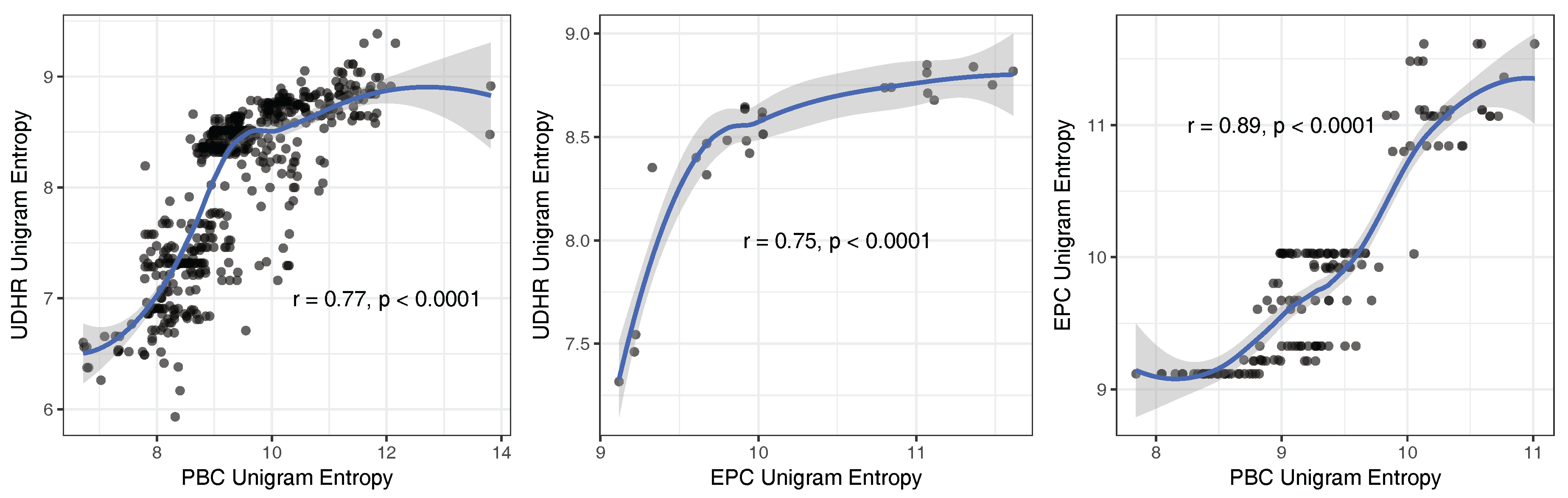
Appendix G. Correlations between PBC, EPC and UDHR Unigram Entropies
References
- Shannon, C.E. A mathematical theory of communication. Bell Syst. Tech. J. 1948, 27, 379–423. [Google Scholar] [CrossRef]
- Shannon, C.E. Prediction and entropy of printed English. Bell Syst. Tech. J. 1951, 30, 50–65. [Google Scholar] [CrossRef]
- Brown, P.F.; Pietra, V.J.D.; Mercer, R.L.; Pietra, S.A.D.; Lai, J.C. An estimate of an upper bound for the entropy of English. Comput. Linguist. 1992, 18, 31–40. [Google Scholar]
- Kontoyiannis, I.; Algoet, P.H.; Suhov, Y.M.; Wyner, A.J. Nonparametric entropy estimation for stationary processes and random fields, with applications to English text. IEEE Trans. Inf. Theory 1998, 44, 1319–1327. [Google Scholar] [CrossRef]
- Gao, Y.; Kontoyiannis, I.; Bienenstock, E. Estimating the entropy of binary time series: Methodology, some theory and a simulation study. Entropy 2008, 10, 71–99. [Google Scholar] [CrossRef]
- Schürmann, T.; Grassberger, P. Entropy estimation of symbol sequences. Chaos Interdiscip. J. Nonlinear Sci. 1996, 6, 414–427. [Google Scholar] [CrossRef] [PubMed]
- Behr, F.H.; Fossum, V.; Mitzenmacher, M.; Xiao, D. Estimating and comparing entropies across written natural languages using PPM compression. In Proceedings of the DCC 2003 Data Compression Conference, Snowbird, UT, USA, 25–27 March 2003; p. 416. [Google Scholar]
- Montemurro, M.A.; Zanette, D.H. Universal entropy of word ordering across linguistic families. PLoS ONE 2011, 6, e19875. [Google Scholar] [CrossRef] [PubMed]
- Montemurro, M.A.; Zanette, D.H. Complexity and universality in the long-range order of words. In Creativity and Universality in Language; Springer: Berlin/Heidelberg, Germany, 2016; pp. 27–41. [Google Scholar]
- Koplenig, A.; Meyer, P.; Wolfer, S.; Müller-Spitzer, C. The statistical trade-off between word order and word structure–Large-scale evidence for the principle of least effort. PLoS ONE 2017, 12, e0173614. [Google Scholar] [CrossRef] [PubMed]
- Takahira, R.; Tanaka-Ishii, K.; Dębowski, Ł. Entropy Rate Estimates for Natural Language—A New Extrapolation of Compressed Large-Scale Corpora. Entropy 2016, 18, 364. [Google Scholar] [CrossRef]
- Bentz, C.; Verkerk, A.; Kiela, D.; Hill, F.; Buttery, P. Adaptive communication: Languages with more non-native speakers tend to have fewer word forms. PLoS ONE 2015, 10, e0128254. [Google Scholar] [CrossRef] [PubMed]
- Ehret, K.; Szmrecsanyi, B. An information-theoretic approach to assess linguistic complexity. In Complexity and Isolation; Baechler, R., Seiler, G., Eds.; de Gruyter: Berlin, Germany, 2016. [Google Scholar]
- Bentz, C. The Low-Complexity-Belt: Evidence for large-scale language contact in human prehistory? In Proceedings of the 11th International Conference (EVOLANG11) on The Evolution of Language, New Orleans, LA, USA, 21 March 2016. [Google Scholar]
- Juola, P. Measuring linguistic complexity: The morphological tier. J. Quant. Linguist. 1998, 5, 206–213. [Google Scholar] [CrossRef]
- Juola, P. Assessing linguistic complexity. In Language Complexity: Typology, Contact, Change; Miestamo, M., Sinnemäki, K., Karlsson, F., Eds.; John Benjamins: Amsterdam, The Netherlands, 2008; pp. 89–108. [Google Scholar]
- Gerlach, M.; Font-Clos, F.; Altmann, E.G. Similarity of symbol frequency distributions with heavy tails. Phys. Rev. X 2016, 6, 021009. [Google Scholar] [CrossRef]
- Bentz, C.; Berdicevskis, A. Learning pressures reduce morphological complexity: Linking corpus, computational and experimental evidence. In Proceedings of the Workshop on Computational Linguistics for Linguistic Complexity (CL4LC), 26th International Conference on Computational Linguistics, Osaka, Japan, 11 December 2016. [Google Scholar]
- Bochkarev, V.; Solovyev, V.; Wichmann, S. Universals versus historical contingencies in lexical evolution. J. R. Soc. Interface 2014, 11, 20140841. [Google Scholar] [CrossRef] [PubMed]
- Rao, R.P.N.; Yadav, N.; Vahia, M.N.; Joglekar, H.; Adhikari, R.; Mahadevan, I. Entropic evidence for linguistic structure in the Indus script. Science 2009, 324, 1165. [Google Scholar] [CrossRef] [PubMed]
- Rao, R.P.N. Probabilistic analysis of an acient undeciphered script. Computer 2010, 43, 76–80. [Google Scholar] [CrossRef]
- Sproat, R. A statistical comparison of written language and nonlinguistic symbol systems. Language 2014, 90, 457–481. [Google Scholar] [CrossRef]
- Rao, R.P.; Yadav, N.; Vahia, M.N.; Joglekar, H.; Adhikari, R.; Mahadevan, I. Entropy, the Indus script, and language: A reply to R. Sproat. Comput. Linguist. 2010, 36, 795–805. [Google Scholar] [CrossRef]
- Piantadosi, S.T.; Tily, H.; Gibson, E. Word lengths are optimized for efficient communication. Proc. Natl. Acad. Sci. USA 2010, 108, 3526–3529. [Google Scholar] [CrossRef] [PubMed]
- Mahowald, K.; Fedorenko, E.; Piantadosi, S.T.; Gibson, E. Info/information theory: Speakers choose shorter words in predictive contexts. Cognition 2013, 126, 313–318. [Google Scholar] [CrossRef] [PubMed]
- Ferrer-i Cancho, R.; Bentz, C.; Seguin, C. Compression and the origins of Zipf’s law of abbreviation. arXiv, 2015; arXiv:1504.04884. [Google Scholar]
- Bentz, C.; Ferrer-i-Cancho, R. Zipf’s law of abbreviation as a language universal. In Proceedings of the Leiden Workshop on Capturing Phylogenetic Algorithms for Linguistics, Leiden, The Netherlands, 26–30 October 2015; Bentz, C., Jäger, G., Yanovich, I., Eds.; University of Tübingen: Tübingen, Germany, 2016. [Google Scholar]
- Futrell, R.; Mahowald, K.; Gibson, E. Quantifying word order freedom in dependency corpora. In Proceedings of the Third International Conference on Dependency Linguistics (Depling 2015), Uppsala, Sweden, 24–26 August 2015; pp. 91–100. [Google Scholar]
- Ackerman, F.; Malouf, R. Morphological organization: The low conditional entropy conjecture. Language 2013, 89, 429–464. [Google Scholar] [CrossRef]
- Milin, P.; Kuperman, V.; Kostic, A.; Baayen, R.H. Paradigms bit by bit: An information theoretic approach to the processing of paradigmatic structure in inflection and derivation. In Analogy in Grammar: Form and Acquisition; Blevins, J.P., Blevins, J., Eds.; Oxford University Press: Oxford, UK, 2009; pp. 214–252. [Google Scholar]
- Levy, R. Expectation-based syntactic comprehension. Cognition 2008, 106, 1126–1177. [Google Scholar] [CrossRef] [PubMed]
- Jaeger, T.F. Redundancy and reduction: Speakers manage syntactic information density. Cognit. Psychol. 2010, 61, 23–62. [Google Scholar] [CrossRef] [PubMed]
- Fenk, A.; Fenk, G. Konstanz im Kurzzeitgedächtnis-Konstanz im sprachlichen Informationsfluß. Z. Exp. Angew. Pshychol. 1980, 27, 400–414. [Google Scholar]
- Fenk-Oczlon, G. Familiarity, information flow, and linguistic form. In Frequency and the Emergence of Linguistic Structure; Bybee, J.L., Hopper, P.J., Eds.; John Benjamins: Amsterdam, The Netherlands, 2001; pp. 431–448. [Google Scholar]
- Ferrer-i Cancho, R.; del Prado Martín, F.M. Information content versus word length in random typing. J. Stat. Mech. Theory Exp. 2011, L12002. [Google Scholar] [CrossRef]
- Ferrer-i Cancho, R.; Dębowski, Ł.; del Prado Martín, F.M. Constant conditional entropy and related hypotheses. J. Stat. Mech. Theory Exp. 2013, L07001. [Google Scholar] [CrossRef]
- Ferrer-i-Cancho, R.; Díaz-Guilera, A. The global minima of the communicative energy of natural communication systems. J. Stat. Mech. Theory Exp. 2007, 2007, P06009. [Google Scholar]
- Ferrer-i-Cancho, R.; Solé, R.V. Least effort and the origins of scaling in human language. Proc. Natl. Acad. Sci. USA 2003, 100, 788–791. [Google Scholar] [CrossRef] [PubMed]
- Ferrer-i-Cancho, R. Zipf’s law from a communicative phase transition. Eur. Phys. J. B 2005, 47, 449–457. [Google Scholar] [CrossRef]
- Ferrer-i-Cancho, R. The optimality of attaching unlinked labels to unlinked meanings. Glottometrics 2016, 36, 1–16. [Google Scholar]
- Berger, A.L.; Pietra, V.J.D.; Pietra, S.A.D. A maximum entropy approach to natural language processing. Comput. Linguist. 1996, 22, 39–71. [Google Scholar]
- Och, F.J.; Ney, H. Discriminative training and maximum entropy models for statistical machine translation. In Proceedings of the 40th Annual Meeting on Association for Computational Linguistics, Philadelphia, PA, USA, 7–12 July 2002; pp. 295–302. [Google Scholar]
- Herbelot, A.; Ganesalingam, M. Measuring semantic content in distributional vectors. In Proceedings of the 51st Annual Meeting of the Association for Computational Linguistics, Short Papers (ACL Short Papers 2013), Sofia, Bulgaria, 4–9 August 2013; pp. 440–445. [Google Scholar]
- Padó, S.; Palmer, A.; Kisselew, M.; Šnajder, J. Measuring Semantic Content To Assess Asymmetry in Derivation. In Proceedings of the Workshop on Advances in Distributional Semantics, London, UK, 14 April 2015. [Google Scholar]
- Santus, E.; Lenci, A.; Lu, Q.; Im Walde, S.S. Chasing Hypernyms in Vector Spaces with Entropy. In Proceedings of the 14th Conference of the European Chapter of the Association for Computational Linguistics, Gothenburg, Sweden, 26–30 April 2014; pp. 38–42. [Google Scholar]
- Resnik, P. Using information content to evaluate semantic similarity in a taxonomy. In Proceedings of the IJCAI’95 Proceedings of the 14th International Joint Conference on Artificial Intelligence, Montreal, QC, Canada, 20–25 August 1995; Volume 1, pp. 448–453. [Google Scholar]
- Boon, M. Information density, Heaps’ Law, and perception of factiness in news. In Proceedings of the ACL Workshop on Language Technology and Computational Social Science (ACL LACSS 2014), Baltimore, MD, USA, 26 June 2014; p. 33. [Google Scholar]
- Stetson, P.D.; Johnson, S.B.; Scotch, M.; Hripcsak, G. The sublanguage of cross-coverage. Proc. AMIA Symp. 2002, 2002, 742–746. [Google Scholar]
- McFarlane, D.J.; Elhadad, N.; Kukafka, R. Perplexity analysis of obesity news coverage. AMIA Annu. Symp. Proc. 2009, 2009, 426–430. [Google Scholar] [PubMed]
- Zhang, Y.; Kordoni, V.; Villavicencio, A.; Idiart, M. Automated multi-word expression prediction for grammar engineering. In Proceedings of the Workshop on Multiword Expressions: Identifying and Exploiting Underlying Properties, Association for Computational Linguistics, Sydney, Australia, 23 July 2006; pp. 36–44. [Google Scholar]
- Ramisch, C.; Schreiner, P.; Idiart, M.; Villavicencio, A. An evaluation of methods for the extraction of multi-word expressions. In Proceedings of the LREC Workshop-Towards a Shared Task for Multiword Expressions (MWE 2008), Marrakech, Morocco, 1 June 2008; pp. 50–53. [Google Scholar]
- Nemenman, I.; Shafee, F.; Bialek, W. Entropy and inference, revisited. Adv. Neural Inf. Process. Syst. 2002, 1, 471–478. [Google Scholar]
- Kalimeri, M.; Constantoudis, V.; Papadimitriou, C.; Karamanos, K.; Diakonos, F.K.; Papageorgiou, H. Entropy analysis of word-length series of natural language texts: Effects of text language and genre. Int. J. Bifurc. Chaos 2012, 22, 1250223. [Google Scholar] [CrossRef]
- Koehn, P. Europarl: A parallel corpus for statistical machine translation. In Proceedings of the tenth Machine Translation Summit, Phuket, Thailand, 12–16 September 2005; Volume 5, pp. 79–86. [Google Scholar]
- Mayer, T.; Cysouw, M. Creating a massively parallel Bible corpus. In Proceedings of the Ninth International Conference on Language Resources and Evaluation (LREC-2014), Reykjavik, Iceland, 26–31 May 2014; Calzolari, N., Choukri, K., Declerck, T., Loftsson, H., Maegaard, B., Mariani, J., Moreno, A., Odijk, J., Piperidis, S., Eds.; European Language Resources Association (ELRA): Paris, France, 2014; pp. 3158–3163. [Google Scholar]
- Haspelmath, M. The indeterminacy of word segmentation and the nature of morphology and syntax. Folia Linguist. 2011, 45, 31–80. [Google Scholar] [CrossRef]
- Wray, A. Why are we so sure we know what a word is? In The Oxford Handbook of the Word; Taylor, J., Ed.; Oxford University Press: Oxford, UK, 2014; Chapter 42. [Google Scholar]
- Geertzen, J.; Blevins, J.P.; Milin, P. Informativeness of linguistic unit boundaries. Ital. J. Linguist. 2016, 28, 25–47. [Google Scholar]
- Dębowski, Ł. Consistency of the plug-in estimator of the entropy rate for ergodic processes. In Proceedings of the 2016 IEEE International Symposium on Information Theory (ISIT), Barcelona, Spain, 10–15 July 2016; pp. 1651–1655. [Google Scholar]
- Jiao, J.; Venkat, K.; Han, Y.; Weissman, T. Minimax estimation of functionals of discrete distributions. IEEE Trans. Inf. Theory 2015, 61, 2835–2885. [Google Scholar] [CrossRef]
- Lesne, A.; Blanc, J.L.; Pezard, L. Entropy estimation of very short symbolic sequences. Phys. Rev. E 2009, 79, 046208. [Google Scholar] [CrossRef] [PubMed]
- Basharin, G.P. On a statistical estimate for the entropy of a sequence of independent random variables. Theory Probab. Appl. 1959, 4, 333–336. [Google Scholar] [CrossRef]
- Hausser, J.; Strimmer, K. Entropy inference and the James–Stein estimator, with application to nonlinear gene association networks. J. Mach. Learn. Res. 2009, 10, 1469–1484. [Google Scholar]
- Shannon, C.E.; Weaver, W. The Mathematical Theory of Communication; The University of Illinois Press: Urbana, IL, USA, 1949. [Google Scholar]
- Harris, B. The statistical estimation of entropy in the non-parametric case. In Topics in Information Theory; Csiszar, I., Ed.; North-Holland: Amsterdam, The Netherlands, 1975; pp. 323–355. [Google Scholar]
- Chomsky, N. Aspects of the Theory of Syntax; MIT Press: Cambridge, MA, USA, 1965. [Google Scholar]
- Baroni, M. Distributions in text. In Corpus Linguistics. An international handbook; Lüdeling, A., Kytö, M., Eds.; De Gruyter: Berlin, Germany, 2009; pp. 803–821. [Google Scholar]
- Ferrer, R.; Solé, R.V. Two Regimes in the Frequency of Words and the Origins of Complex Lexicons: Zipf ’s Law Revisited. J. Quant. Linguist. 2001, 8, 165–173. [Google Scholar] [CrossRef]
- Gerlach, M.; Altmann, E.G. Stochastic model for the vocabulary growth in natural languages. Phys. Rev. X 2013, 3, 021006. [Google Scholar] [CrossRef]
- Petersen, A.M.; Tenenbaum, J.; Havlin, S.; Stanley, H.E.; Perc, M. Languages cool as they expand: Allometric scaling and the decreasing need for new words. Sci. Rep. 2012, 2, 943. [Google Scholar] [CrossRef] [PubMed]
- Manning, C.D.; Schütze, H. Foundations of Statistical Natural Language Processing; MIT Press: Cambridge, MA, USA, 1999; Chapter 5. [Google Scholar]
- Montemurro, M.; Pury, P.A. Long-range fractal correlations in literary corpora. Fractals 2002, 10, 451–461. [Google Scholar] [CrossRef]
- Cover, T.M.; Thomas, J.A. Elements of Information Theory; John Wiley and Sons: Hoboken, NJ, USA, 2006. [Google Scholar]
- Ziv, J.; Lempel, A. A universal algorithm for sequential data compression. IEEE Trans. Inf. Theory 1977, 23, 337–343. [Google Scholar] [CrossRef]
- Ziv, J.; Lempel, A. Compression of individual sequences via variable-rate coding. IEEE Trans. Inf. Theory 1978, 24, 530–536. [Google Scholar] [CrossRef]
- Hausser, J.; Strimmer, K. Entropy: Estimation of Entropy, Mutual Information and Related Quantities, R Package Version 1.2.1; 2014. Available online: https://CRAN.R-project.org/package=entropy (accessed on 13 June 2017).
- Bates, D.; Mächler, M.; Bolker, B.; Walker, S. Fitting Linear Mixed-Effects Models Using lme4. J. Stat. Softw. 2015, 67, 1–48. [Google Scholar] [CrossRef]
- Hammarström, H.; Forkel, R.; Haspelmath, M.; Bank, S. Glottolog 2.7; Max Planck Institute for the Science of Human History: Jena, Germany, 2016. [Google Scholar]
- Kirby, S.; Tamariz, M.; Cornish, H.; Smith, K. Compression and communication in the cultural evolution of linguistic structure. Cognition 2015, 141, 87–102. [Google Scholar] [CrossRef] [PubMed]
- Ferrer-i-Cancho, R. Optimization models of natural communication. arXiv, 2014; arXiv:1412.2486. [Google Scholar]
- Bentz, C.; Ruzsics, T.; Koplenig, A.; Samaržić, T. A comparison between morphological complexity measures: typological data vs. language corpora. In Proceedings of the Workshop on Computational Linguistics for Linguistic Complexity (CL4LC), 26th International Conference on Computational Linguistics, Osaka, Japan, 11 December 2016. [Google Scholar]
- Baayen, H.R. Word Frequency Distributions; Kluwer: Dordrecht, The Netherlands; Boston, MA, USA; London, UK, 2001. [Google Scholar]
- Agresti, A.; Hitchcock, D.B. Bayesian inference for categorical data analysis. Stat. Methods Appl. 2005, 14, 297–330. [Google Scholar] [CrossRef]
- Chao, A.; Shen, T.J. Nonparametric estimation of Shannon’s index of diversity when there are unseen species in sample. Environ. Ecol. Stat. 2003, 10, 429–443. [Google Scholar] [CrossRef]


| Corpus | Register | Size * | Mean Size * | Texts | Lang |
|---|---|---|---|---|---|
| EPC | Political | ca. 21 M | ca. 1 M | 21 | 21 |
| PBC | Religious | ca. 430 M | ca. 290 K | 1525 | 1137 |
| UDHR | Legal | ca. 500 K | ca. 1.3 K | 370 | 341 |
| Total: | ca. 450 M | 1916 | 1259 |
© 2017 by the authors. Licensee MDPI, Basel, Switzerland. This article is an open access article distributed under the terms and conditions of the Creative Commons Attribution (CC BY) license (http://creativecommons.org/licenses/by/4.0/).
Share and Cite
Bentz, C.; Alikaniotis, D.; Cysouw, M.; Ferrer-i-Cancho, R. The Entropy of Words—Learnability and Expressivity across More than 1000 Languages. Entropy 2017, 19, 275. https://doi.org/10.3390/e19060275
Bentz C, Alikaniotis D, Cysouw M, Ferrer-i-Cancho R. The Entropy of Words—Learnability and Expressivity across More than 1000 Languages. Entropy. 2017; 19(6):275. https://doi.org/10.3390/e19060275
Chicago/Turabian StyleBentz, Christian, Dimitrios Alikaniotis, Michael Cysouw, and Ramon Ferrer-i-Cancho. 2017. "The Entropy of Words—Learnability and Expressivity across More than 1000 Languages" Entropy 19, no. 6: 275. https://doi.org/10.3390/e19060275
APA StyleBentz, C., Alikaniotis, D., Cysouw, M., & Ferrer-i-Cancho, R. (2017). The Entropy of Words—Learnability and Expressivity across More than 1000 Languages. Entropy, 19(6), 275. https://doi.org/10.3390/e19060275