
Horton Ratios Link Self-Similarity with Maximum Entropy of Eco-Geomorphological Properties in Stream Networks

1
Department of Biology, 1 University of New Mexico, MSC03-2020, Albuquerque, NM 87131, USA
2
Department of Civil, Environmental and Architectural Engineering and Cooperative Institute for Research in Environmental Sciences, University of Colorado, Boulder, CO 80309, USA
*
Author to whom correspondence should be addressed.
Entropy 2017, 19(6), 249; https://doi.org/10.3390/e19060249
Submission received: 17 March 2017
/
Revised: 25 May 2017
/
Accepted: 27 May 2017
/
Published: 30 May 2017
(This article belongs to the Special Issue Entropy in Landscape Ecology)
Abstract
:Stream networks are branched structures wherein water and energy move between land and atmosphere, modulated by evapotranspiration and its interaction with the gravitational dissipation of potential energy as runoff. These actions vary among climates characterized by Budyko theory, yet have not been integrated with Horton scaling, the ubiquitous pattern of eco-hydrological variation among Strahler streams that populate river basins. From Budyko theory, we reveal optimum entropy coincident with high biodiversity. Basins on either side of optimum respond in opposite ways to precipitation, which we evaluated for the classic Hubbard Brook experiment in New Hampshire and for the Whitewater River basin in Kansas. We demonstrate that Horton ratios are equivalent to Lagrange multipliers used in the extremum function leading to Shannon information entropy being maximal, subject to constraints. Properties of stream networks vary with constraints and inter-annual variation in water balance that challenge vegetation to match expected resource supply throughout the network. The entropy-Horton framework informs questions of biodiversity, resilience to perturbations in water supply, changes in potential evapotranspiration, and land use changes that move ecosystems away from optimal entropy with concomitant loss of productivity and biodiversity.
Keywords:
Budyko; coupled eco-hydrology; Horton law; networks; scaling; Strahler streams; vegetation1. Introduction
Energy expenditure is fundamental to the development of an ecosystem’s structure, function, resilience, sustainability, and species diversity [1,2,3,4]. Several consistent goal functions [5,6,7] admit that ecosystems organize to dissipate energy at maximum rate with minimal work per volume [8], subject to constraints of land area, size of the species pool, densities of individuals, and metabolic rates [9,10]. These categories of constraint constitute many modes of heat transport and thereby combinations by which the work accomplished balances the given heat flow [5]. Parsimony allows solutions to the problem of energy dissipation as the outcome of reaching the most probable state, indicated by a maximum value of Shannon entropy [11].
For total global energy dissipation to proceed, modes of dissipation at finer scales of continents, mountain ranges, catchments, hillslopes, and individual plants participate in coupled networks that operate to varying degrees, day and night. Energy dissipation in each parcel of land adds to the total according to entropy being an extensive property. Thus, the partitioning of entropy through space is inherently a matter of scaling in networks of streams characterized by ubiquitous Horton relations and laws that relate basin area to ecohydrological properties [12]. Horton laws characterize the availability of water in successively larger basins, channels, and riparian areas.
Kleidon [13] conceptualizes the global system as coupled circuits composed of storages and resistors wherein water and carbon cycles depart from thermodynamic equilibrium. Thermodynamic arguments define a requisite spatial scale at which energy dissipation dominates entropy to produce fluvial networks [14]. As the conduits for flow of water and materials, rivers and streams that stretch ~8.82 × 10¹⁰ m across the globe [15] divide landscapes into hierarchies of channels, hillslopes, and ridges that establish topographical and environmental support. Leopold and Langbein [16] consider entropy an organizing principle in hydrology, without considering vegetation. In the water-limited Rio Puerco basin in New Mexico, entropy explains the spatial distribution of functional types of vegetation as the most probable state, on the basis that ecological entropy production is equivalent to maximizing canopy photosynthesis [17]. Synthesis is needed to understand entropy production by coupled hydro-geomorphological and ecological processes that establish spatial variation in temperature, moisture, and consequently production and biodiversity.
Entropy is an extensive property, being additive across space. With watershed basins as natural units, and under the assumption that inputs balance outputs at annual time scales, we assumed precipitation (PPT) is the sum of actual evapotranspiration (ET), and flow (Q) out the main drainage channel. We focused on Shannon information entropy calculated from the two fractions, ET/PPT and Q/PPT. By closing budgets within basins, we examined the partitioning of input energy between dissipated and free components across a range of climates, examined the active role of vegetation in the partitioning, and detailed the manner of entropy partitioning among sub-basins in scale-dependent fashion. Accordingly, we hypothesized that observed configurations of sub-basins, stream numbers and lengths, vegetated area along channels, and the number of species per stream, will be the most probable arrangements of parts among the whole.
Coupling between ecological and hydrological systems is subject to: (1) Pervasive biological regularities; and (2) contingencies that restrict ecological activity in deference to abiotic modes of dissipation. In ecological systems composed of individuals and populations, regularity takes allometric form, or quarter-power scaling between body mass and virtually all aspects of life [18]. Allometry gives rise to invariant properties of energy use per unit area [19,20,21]. For example, Damuth’s [22] law for faunal metabolic power per unit area (D) and an equivalent temperature-corrected relation for plants [23], depends on individual body mass (M). Population density and energy use per individual vary as mass to the −3/4 and 3/4 power, respectively, thereby . Energy use by plants that vary the seven orders of magnitude in individual mass averages 10,000 W/km2 [23]. This uniformity agrees with Field et al.’s [24] observation of a narrow range in light-use efficiency, from 0.135 to 0.354 g·C·MJ−1 of photosynthetically active radiation, observed from deserts to broadleaf evergreen forests. Thus, invariance implies that a ~25-fold variation in net primary production [25] is explained by fluctuations in temperature, radiation, and water availability with season, latitude and topography.
Contingencies at subannual time scales restrict ecological work to less than 100% of input energy [26]. Vegetation partitions precipitation into flow and evapotranspiration even in basins of 1000 km2 or less [27,28]. Rainfall may be out of synchrony with seasonal and temperature-dependent metabolic demand, so water escapes as runoff or re-enters the atmosphere by evaporation at a maximum rate [29,30]. To protect against photo-oxidation, plants lose through photorespiration one of every six carbon atoms captured by photosynthesis [31]. This lost carbon could otherwise be invested in roots and shoots with concomitant diversion from flow and evaporation. In general, vegetation composition and functional types configure to match the frequency spectrum of energy supply [32,33] subject to physiological constraints. Inherent tradeoffs between dissipation as flow versus evapotranspiration brings into question whether energy dissipation always reaches the theoretical maximum.
We examined four hypotheses to trace out how landscapes and stream networks partition precipitation into flow and evapotranspiration. First, we ascertained from Budyko’s [34] theory how net radiation, or equivalently potential evapotranspiration, and rainfall set entropy for a given climate, from which we hypothesized maximum entropy appears as an optimum. Second, to study entropy as an extensive property we analyzed basin-wide water balance for systems near and far from optimum entropy and showed opposite effects of rainfall rate on entropy, suggesting that vegetation change enables systems to move toward higher biodiversity. Third, with our Lagrange equivalence hypothesis (LEH), we established one-to-one correspondence between constraints that ensure Shannon entropy is maximal and the scaling exponent of classic Horton relations. Fourth, we evaluated the network entropy hypothesis (NEH) by numerical experimentation for a set of Horton laws to assess how closely vegetation reaches maximum entropy in a network of 13,062 streams. The hypotheses bridge between global energetics and the coupled systems by which energy is dissipated across space, down to scales as small as individual organisms.
1.1. Optimal Entropy Hypothesis (OEH)
Bejan and Lorente [7] posit the constructal law wherein optimal structures emerge that facilitate maximum flow, subject to constraint. Accordingly, configurations of streams and vegetation within a basin share the burden of dissipating incoming radiation and precipitation. Because free energy is lowest where the product of entropy and input energy is highest, we expect maximum dissipation at maximum entropy, which implies an optimal combination of energy and water inputs.
We developed our optimal entropy hypothesis (OEH) from Budyko’s theory [28,34,35]. Budyko arranged global climates and biomes according to the ratio of net radiation to rainfall, to give aridity index B. These factors interact to yield actual evapotranspiration, as described by the geometric mean of two functions, one describing the effect of precipitation and a second the effect of radiation,
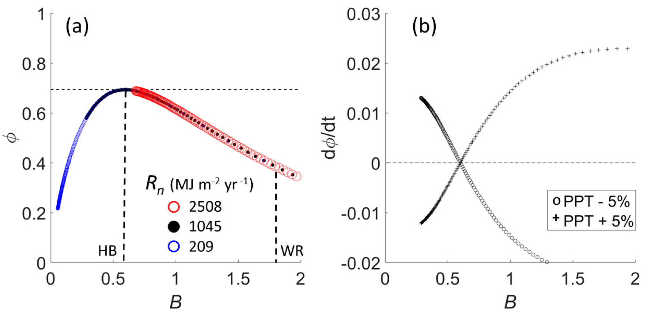
where Rn is net radiation, r is rainfall, and L is the latent heat of vaporization by which rainfall is converted to units of energy [34]. The portion of precipitation manifest as ET increases monotonically with aridity index. Under the assumption that r = Q + ET, we normalized runoff and flow by rainfall to obtain two probabilities. These gave Shannon information entropy that reaches unconstrained maximum log(2) at optimum B* = 0.6 (Figure 1a). Because B and the fractions Q/r, and ET/r are dimensionless, entropy as a function of B is universal for all combinations of net radiation and rainfall (see [36]). Varying Rn to include values typical of tundra, mid-latitude deciduous forests, and subtropical biomes merely translates entropies for a given set of rainfall rates along the curve. Hereafter we replace symbol r with the symbol for precipitation, PPT.
Perturbing rainfall rates by ±5% changes entropy in opposite ways for systems on either side of B* (Figure 1b). Thus, we hypothesized that energy-limited (humid) systems reach maximum entropy under drying conditions while water-limited (arid) systems approach maximum entropy in years of high rainfall. We expect coupled systems to configure vegetation within stream networks to reach the most likely state of maximum entropy allowed by rainfall. Due to self-similar topology, stream networks concentrate moisture in higher order streams through contributions from lower-order side branches [37]. We elaborate this idea with the next two hypotheses.
1.2. Lagrange Equivalence Hypothesis
Stream networks and sub-basins form scale-invariant branching hierarchies indexed by Horton–Strahler orders, ω = 1, 2, …, Ω [38]. Theory of scaling in stream networks has an assumption of strict self-similarity [12,39,40]. In ubiquitous empirical Horton laws observed for Horton ratios associated with basin areas and stream numbers [12], a Horton ratio, , describes the exponential increase (or decrease) in a variable, X, from one order to the next. In exponential form, with prefactor c and . A Horton law with exponent γ relates the Horton ratio of basin area to the Horton ratio of another variable, as .
A Horton ratio for Shannon entropy of seven riparian vegetation types along 13,062 streams in the Whitewater River basin in Kansas [41] indicates that resource availability increases with stream order. We hypothesized that Horton laws and maximum entropy are directly related; indeed we claim parameter b for stream numbers is identical to the Lagrange multiplier by which the Shannon function is maximal for a set of constraints [11].
1.3. Network Entropy Hypothesis
Horton scaling implies coherence within Strahler networks, wherein fluxes at each location are both differentiating and integrating of inputs via physical and ecological processes, resulting in non-local water balance at all scales [37]. Riparian vegetation participates in the balance by populating the basin sufficiently to match expected resource availability. Local over-stocking of vegetation will deplete water supply for downstream plants, while understocking will enable proliferation of plants downstream. Vegetation demand for water can adjust to meet supply via the number of streams occupied, the lengths of occupied streams, the areal cover along stream channels, and the number of vegetation types per stream. Assuming these properties obey Horton scaling, we expect exponents in corresponding Horton laws will relate basin area to vegetation at maximum total entropy summed across all orders.
2. Materials and Methods
We re-examined the classic vegetation removal experiment of an energy-limited watershed at Hubbard Brook, New Hampshire [42], to establish maximum information entropy as the attractive state, in keeping with the optimal entropy hypothesis (OEH). We developed an analogous budget for the water-limited Whitewater River basin and examined the classic Horton scaling of eco-hydrological properties [41] to show homology between Horton laws and Lagrange multipliers used in the extremum function that defines Shannon entropy as maximal.
2.1. Study Watersheds
We used annual precipitation and streamflow at Hubbard Brook Experimental Forest, New Hampshire [42] to assess entropy, dissipated energy, and free energy of this energy-limited system. The classic study involved the experimental removal of vegetation from an entire watershed. During the experiment, mean annual precipitation of 1230 mm was evenly distributed throughout the year, but peak streamflows occurred in April and November with minimal deep infiltration, thereby supporting the assumption that PPT = Q + ET. Likens et al. [42] report annual measurements for 1 June–31 May (beginning in 1963–1964 through 1967–1968) for five control watersheds and one treatment (Watershed 2, 15.6 ha). From latitude (43.9° N) and [1], the lower estimate of potential evapotranspiration (PET) was ~850 mm/yr. Based on highest annual PPT, the corresponding aridity index was ~0.6 (Figure 1a).
Land cover in the more arid Whitewater River basin (1080 km2) is 85% agricultural as a mixture of cultivated (58.6%) and prairie managed for grazing (25.5%). Forests occupy 6.1%, predominantly in riparian areas and flood plains, where soil moisture recharge through stream channels is adequate to support trees [43]. Dunn et al. [41] describe delineation of stream networks for characterization of Horton laws and the mapping of seven riparian vegetation types [44]. Vegetation types and areas were tallied within 100-m wide buffers along stream channels. Here, we restricted vegetation data to the “exclusive” subset [41] where buffers did not overlap. This avoided difficulties of ascribing vegetation to order in overlap zones.
We developed long-term water balance for the Whitewater River basin from precipitation records for El Dorado and Potwin, Kansas. El Dorado is located near USGS gauge 07147070 at Towanda, on the order-7 stream. We used daily flows (n = 15,706) recorded at Towanda to construct water balance for years 1962–2004, contemporaneous with vegetation data. We multiplied daily mean flows (m3/s) by seconds per day to obtain daily volumes (m3) and summed throughout the year for the annual volume. Dividing volume by the basin area gave an annual rate (mm/yr). We used annual precipitation at El Dorado to obtain basin-wide ET (mm/yr) by subtraction. Our assumption of zero infiltration at sufficiently long time scales does not preclude sub-annual infiltration to satisfy vegetation demand. We compared median annual PPT to the sum of median annual Q plus median annual ET, which would be equal for zero infiltration. The sum was 95% of median PPT, supporting the assumption that a trivial fraction of PPT was unaccounted for in the long-term water balance. Potwin is 24 km northwest of the gauge, which allowed testing the assumption of spatially uniform precipitation. From latitude (37.9° N) and [1], PET was ~1500 mm/yr. With mean PPT of 850 mm/yr, the aridity index was ~1.8 (Figure 1a).
2.2. Basin-Wide Entropy and Energy Dissipation
Free energy (F) is the solution to minimizing energy while maximizing entropy, accomplished by setting the ratio of probabilities [45]. It is axiomatic that, by setting k = 1, the Boltzmann probabilities allow for “temperature” to be measured in convenient units of energy. Depth of water is a more natural measure for ecohydrology. Recognizing that a millimeter of water over a square meter is 1 kg, multiplying depth by the latent heat of vaporization (2.450 MJ·kg−1) transforms depth of water to units of energy [34]. The equation for free energy, , posits PPT as input energy, with an amount dissipated. Free energy (F) escapes without fulfilling the potential for work, as when spates deny vegetation water that otherwise could be transpired, or during the non-growing season.
2.3. Lagrange Equivalence Hypothesis
We tested the hypothesis that the Horton relation for stream numbers () is equivalent to maximum entropy, in that exponent b is the Lagrange multiplier, λ, used to derive the Shannon entropy function. Equivalently, the Horton ratio for stream numbers RB = exp(λ).
We defined a set i = ω = 1, 2, … Ω and probabilities pi of having streams each with a “score,” εi, which is order ω = εi. To derive the entropy function to be maximum for a given set of probabilities, the constraint equations are, first, conservation of probability,
and second, expected value of stream order,
To connect Horton scaling to the entropy function, we have Lagrange multipliers α and λ by which to multiply derivatives of the constraint equations, and , respectively. This gives the extremum equation,
which, summed over all i gives total derivative,
As the test, we substituted the known expression for the partial derivative of the Shannon function,
into Equation (3) which gave
or,
which has the same functional form as a Horton relation. Thus, we hypothesized the Lagrange multiplier relates empirical probabilities to stream order with a slope equal to the empirical parameter of the Horton scaling relation.
2.4. Network Entropy Hypothesis and Horton Laws
Dissipation of precipitation as ET and Q in fluvial networks are alternative modes of energy expenditure. We designed a numerical experiment to assess which measures of vegetation couple to the Strahler network through entropy, as defined for the LEH. Unlike a classic Horton law that relates mean values, we examined ratios of nonlinearly scaled variables stream by stream, which allowed the covariance to inform the scaling exponent.
The experiment had two parts. First, as a null model, we estimated the exponents of Horton laws from mean values. This gave exponents . Second, we obtained entropies with explicit reference to order for a wide range of exponent values thereby to identify at which entropy was maximal. The experiment had null hypotheses for exponents, , and for the corresponding entropies, . Inferences for outcomes of the tests are given in Table 1. An alternative hypothesis was that extensive properties of vegetation among Strahler streams are sensitive to basin area, understood as surrogate for resource supply, and that per stream, the network enables higher entropy throughout the basin.
Here, we detail the experimental treatments using Equations (6)–(8). By the LEH, the distribution of expected values for a variable among orders is most probable. In Whitewater River basin, orders 1 through 6 contained complete Strahler streams, whereas the single order-7 stream did not join another order-7, which made it incomplete and ignored for this purpose. A quantity distributed equally among six orders has probability 1/6, which gives uniform distribution and maximum unconstrained entropy
We rearranged the Horton law to define ratios
for each stream (i) of order ω. For the null model, we estimated the exponent in power law form where and are geometric means [46]. This treats the two variables separately, while Equation (6) binds them stream-by-stream, thereby allowing the covariance to affect the exponent.
The extent to which geometric mean ratios are constant with order is the extent to which the distribution is uniform. We normalized each mean by the sum of means to obtain probabilities
which gave Shannon entropy
To test the NEH, we found where entropy reached maximum for comparison to Hmax and to entropy from the null model, . The comparison required bootstrapping, with replacement, total entropy summed across orders, using 250,000 iterations to obtain a stable value for the standard deviation.
3. Results
3.1. Hubbard Brook Vegetation Removal Experiment
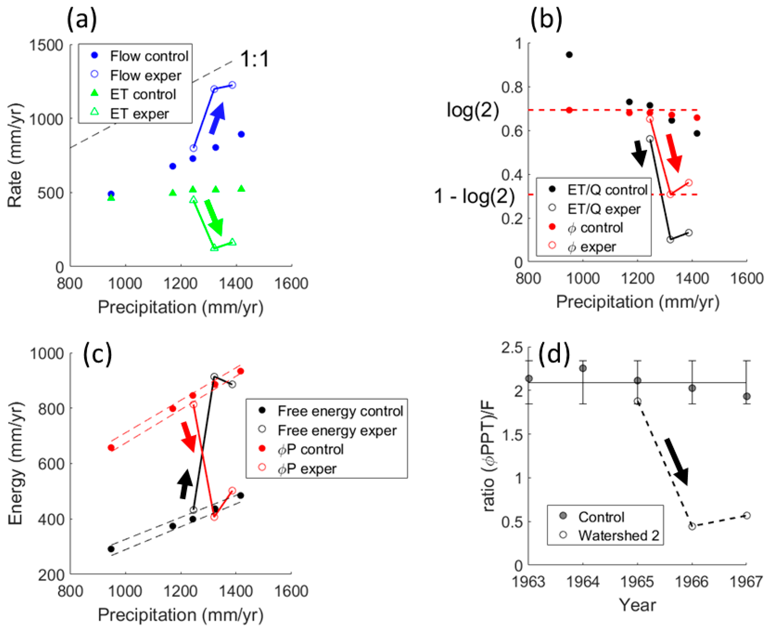
The energy-limited watersheds of Hubbard Brook converted 58% of precipitation to flow, 42% greater than evapotranspiration (Figure 2a). We calculated a lowest feasible value for the Budyko aridity index of B = 0.6, as the ratio of lowest potential evapotranspiration at 44° latitude [1] to highest precipitation measured during the original study [42]. This, in excellent agreement with Budyko [33] expectation (his Figure 103), would place Hubbard Brook at maximum entropy (Figure 1a). A more typical aridity index based on mean annual precipitation would be 900 mm potential evapotranspiration, PET, per 1220 mm PPT, giving B = 0.74. As predicted from the OEH, the ratio ET/Q approached unity at low precipitation, which gave maximum unconstrained entropy (Figure 2b). Experimental removal of vegetation mid-way through water year 1963–1964, followed by two years of herbicide treatment, shifted ET/Q downward (Figure 2b). Entropy of control watersheds centered around the theoretical maximum of log(2) but plunged abruptly after vegetation removal to 1 − log(2).
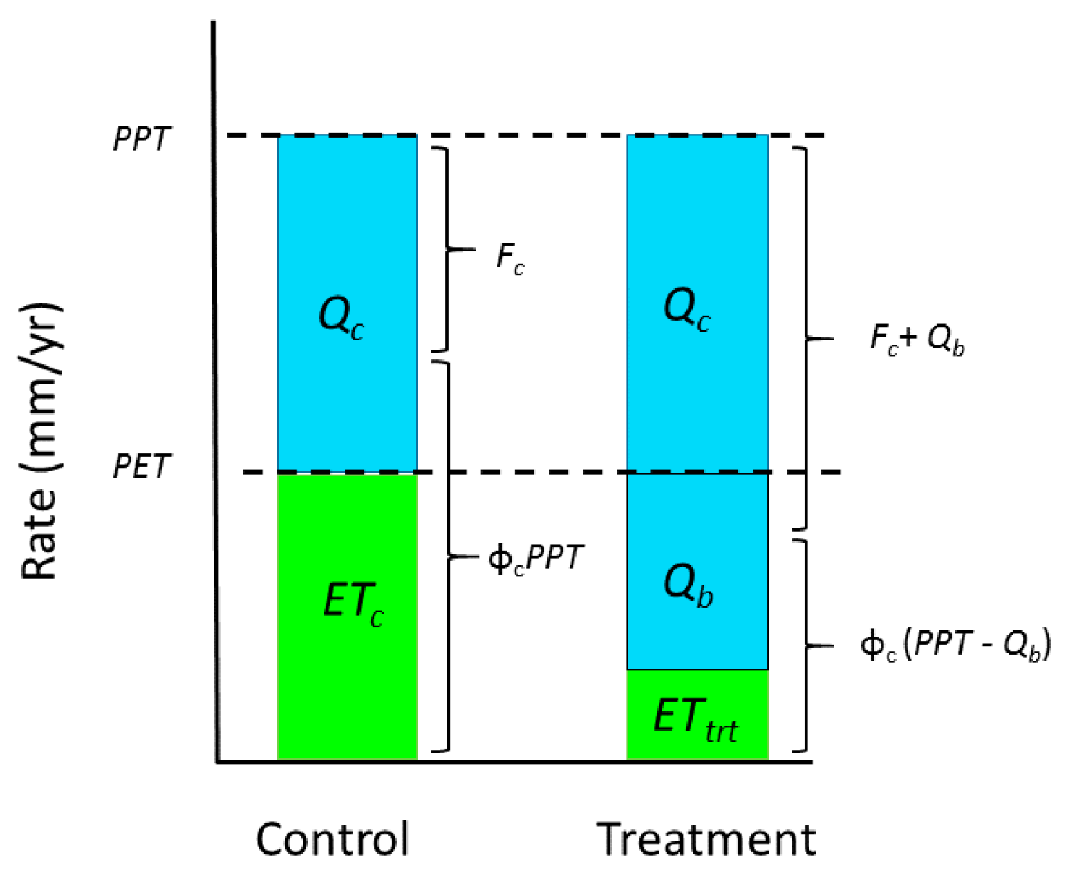
Similarly, vegetation removal flipped the partitioning of precipitation into dissipated energy,PPT, and free energy, PPT(1 − ), corresponding to a 4-fold drop in relative efficiency (Figure 2c,d). The discrete drop in entropy was due to conversion of some ET to flow in the amount Qb = PPT − ETc − Qc, where subscript c denotes control (Figure 3). We assumed that in control watersheds, ET was set by potential evapotranspiration, PET [47]. Entropy allowed ~60% of precipitation to be dissipated (Figure 2c; PPT = 97.25 + 0.595PPT, F[2,3] = 996, P < 0.0001). Removal of vegetation centered the free energy of Watershed 2 on this relation, while in reciprocal fashion, dissipated energy straddled the free energy relation of controls (Figure 2c). Thus, dissipated energy of the treatment watershed complemented the free energy of the controls and vice versa, thereby confirming an active role of vegetation in determining energetics of the system.
3.2. Water Balance for the Whitewater River Basin
Annual precipitation (1954–2005) was uniform across the relatively large basin of Whitewater River. Precipitation at El Dorado, PPTED, tended to be 10 percent higher than at Potwin in years with less than 975 mm, but converged to the 1:1 relation in wetter years (PPTED = 168.48 + 0.858 PPTPot; F[2,50] = 222, P < 0.0001).
On average, 82% of precipitation in the water-limited Whitewater basin was converted to evapotranspiration, consistent with Budyko [34] aridity index ~1.8 (Figure 1a), typical of this geographic location (see Budyko’s [34] Figure 103). Flows and evapotranspiration had power-law dependence with precipitation (Figure 4a; Q = 1.6297 × 10⁻⁶ PPT2.68, F[2,41] = 45.5, P = 3.7 × 10⁻⁸; ET = 7.03 PPT0.68, F[2,41] = 86.3, P = 1.2 × 10⁻¹¹) which compared well with power-law dependence in 11 mid-western basins [48]. In support of the OEH, the ratio ET/Q varied as PPT−2 (Figure 4b) to approach unity with higher precipitation, thereby taking entropy to the unconstrained maximum. As for Hubbard Brook control watersheds, dissipated energy exceeded free energy (Figure 4c) and was linear with precipitation (PPT = −67.03 + 0.7179 PPT, F[2,41] = 1910; P = 5 × 10−36). The steeper slope made Whitewater 20% more effective at dissipating precipitation than Hubbard Brook. Whitewater supported the hypothesis that entropy per volume is minimal (Figure 4d). Entropy per unit flow was highly sensitive in years with below average precipitation, precisely when entropy was below the unconstrained maximum.
3.3. Horton Ratios as Lagrange Multipliers
Number of streams at each order is a special case among eco-hydrological variables because there can be but one value at each order, as opposed to distributions of values. This limits the number of Lagrange multipliers to just two: one for the probability constraint and one for the expected value.
We calculated empirical probabilities of stream orders for all 13,062 streams in Whitewater as . As predicted, the l.h.s. of Equation (4) was a linear function of order (F[2,4] = 10,700; P < 0.0001), with slope λ = 1.52 (0.015 s.e.). This agreed with b obtained as the geometric mean of successive ratios, which gave (0.012 s.e.) The Lagrange multiplier for the probability constraint, (0.057 s.e.) gave c = 0.107, by which the relation passed through the origin.
Restricting stream counts to the 2537 streams occupied by riparian vegetation gave Horton relation (F[2,4] = 272, P < 0.0001). From Equation (4), Lagrange multiplier λ = 1.458 (0.0884 s.e.) supported the LEH, albeit with smaller RB = 4.29 than for the set of all streams, RB = 4.667 (0.0545 s.e.). Intercept α = −2.077 (0.3444 s.e.; t = −6.03, P = 0.004) gave 0.125 as Lagrange multiplier for the probability constraint.
We repeated the second test 100 times, using random subsets of 2537 streams regardless of vegetation occupation and found perfect correlation between parameter b and λ (mean b = 1.488, s.d. 0.136; range 1.238–1.836), which was statistically indistinguishable from parameters of the entire set of streams. Thus, vegetation occupancy was not required to satisfy the LEH.
Richness of vegetation types, stream length, and vegetated area supported the LEH, where was defined using means at each order. These gave significant Horton relations and Lagrange relations with order (P < 0.0001), with perfect agreement between b and λ to at least four decimal places. The four variables, ranked from highest to lowest constraint, were stream number, richness, length, and vegetated area, with λ values 1.52, 1.16 (s.e. 0.104), 0.86 (s.e. 0.049), and 0.28 (s.e. 0.043), respectively.
3.4. Network Entropy Hypothesis and Horton Laws
We related vegetation to basin area under the network entropy hypothesis that exponents of Horton laws taken stream-by-stream correspond to maximum entropy, subject to constraint. In the null model, the number of streams at each order occupied by vegetation, and mean values at each order for lengths of occupied streams, vegetated area, and richness of vegetation types, gave Horton laws . For number of vegetated streams, nω, we fit a power law with geometric mean basin area (, F[2,4] = 5340; P < 0.0001). Length of occupied streams varied as ; F[2,4] = 833, P < 0.00001). Vegetated area of occupied streams (F[2,4] = 691, P < 0.00001). In keeping with exponents typical of the maximum entropy species-area relation [10], richness of types was (F[2,4] = 26.2, P < 0.007, R2 = 0.83).
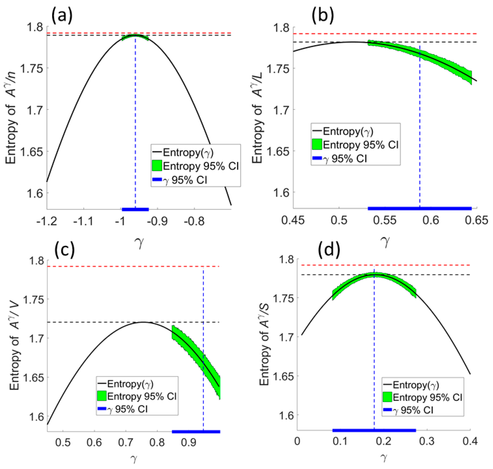
We tested the network entropy hypothesis by experimentally varying exponent values over the 95% confidence of the null exponent and comparing total entropy of the geometric mean ratio, , with the null hypotheses . Null models for number of streams occupied by vegetation and richness of vegetation types supported classic Horton laws being maximum entropy outcomes, given constraint (Figure 5a,d). The NEH was consistent with there being different exponents for number and richness.
The null model for stream length was consistent with the NEH at the low end of the CI, although the most likely value for the null exponent exceeded that of the experimental maximum (Figure 5b), as for vegetation area (Figure 5c). According to Table 1, we inferred that by conditioning the variables stream-by-stream on nonlinearly scaled basin area, entropy was raised above that of the null model.
4. Discussion
Our hypotheses bridged from broad characterizations of climate-related optimum entropy, which is a statement about conditions at a geographic point, to elaborate about spatial scaling of eco-hydrological properties among streams. Sposito’s [49] elucidation of the Budyko equation as scale invariant supports our contention that stream networks of various sizes and orders are manifestations of water and energy relations governed by fundamental rules. Thus, drainage networks can be understood as parts of the globe that participate coherently in energy flow of the whole.
Our demonstration of one-to-one correspondence between classic Horton relations and the principle that information entropy is maximal, given a set of constraints, makes both constructs available for quantifying constraints and the set of options by which coupled systems are able to dissipate potential energy. Support for the Lagrange equivalence hypothesis for stream number established this Horton relation as a maximum entropy outcome, independent of vegetation occupancy, indicating that the stream network is a primary support upon which vegetation organizes simultaneously at multiple scales. The hypothesis had equally strong support for mean values of vegetation properties, commensurate with how strongly each departed from unconstrained maximum entropy. Thus, Horton relations give direct measures of constraint and establish a hierarchy of constraints.
The theory of Horton laws is based on an empirically robust assumption of topological self-similarity [50], which being both simple and stringent, is central to Tokunaga theory [39], wherein the mean number of side branches of streams of one order joining a stream of higher order is a constant ratio. McConnell and Gupta [40] proved a solution of the Tokunaga model that gives Horton ratio for stream number. Raymond et al. [37] elaborate Tokunaga theory to understand the role of low-frequency, large flow events for regulating dissolved organic matter. Their pulse-shunt concept addresses the intermittent, contingent dynamics in multi-scale Strahler networks. The theory should find further application to problems of entropy and energy dissipation across landscapes, perhaps where changes in land use practices alter riparian vegetation cover. We expect it would require wholesale impacts on land cover, as result from herbivore invasions or pathogens, to induce a coherent shift in how energy is partitioned, as for Hubbard Brook (Figure 2).
The extensive nature of entropy and scaling within networks as shown by the network entropy hypothesis may constitute a basis for resilience from the branched network itself. Stream length, richness of vegetation types, and vegetative cover had network entropies below theoretical maximum. Compared to classic Horton laws, network entropy evaluated from stream-by-stream ratios (Equation (6)) provided better sense of how far each variable was below theoretical maximum entropy. None of the entropies reached theoretical maximum of 1.79, indicating that entropy was constrained. However, taking gave the equivalent number of orders required to return the same entropy, were probabilities equal [51]. Thus, even vegetated area would ‘fill’ ~5.6 orders, suggesting it came arbitrarily close to maximum, in keeping with the inherently low sensitivity of entropy to variations in probability [15]. Total entropies departed from theoretical maximum in the order , in same rank order as the Lagrange multipliers ranked from large to small. Taking stream number as example, its large Lagrange multiplier measured the high relevance of the constraint on expected value, as did the proximity of to the theoretical maximum.
Factors such as soil type, agricultural- versus riparian forest-cover on floodplains, and inter-annual variation in rainfall affect erosion rates and meanders [52] that determine stream length. Land cover types could affect entropy through differential responses to inter-annual variability in PPT, which prevents trees especially from having optimal root/shoot ratio each year, thereby imparting temporal trends in streamflow as plantations establish [53].
Remarkably, comparison of Figure 1a with Budyko’s [34] depiction of biomes shows maximum biological diversity at B*, falling off abruptly either side. Since evolutionary change occurs by shifts in gene frequencies at the population level, among sets of individuals, spatially extensive water balance in basins exposes populations to ecohydrological entropy as a potential factor of natural selection, as it reflects the partitioning of input resources differentially into primary production that supports organisms, or otherwise, reduces resource availability. The asymmetry of ecological responses to fluctuations in rainfall either side of B* could drive plant species to diversify by specializing in the many modes of energy dissipation [54], a process that began over 500 million years ago as plants colonized land. The preponderance of the contemporary land surface has higher aridity than optimum, which raises the sensitivity of entropy to fluctuations in rainfall (Figure 1b), of relevance to ongoing selection and species coexistence [55,56].
5. Conclusions
We extended Budyko’s [34] theory to study information entropy as the partitioning of rainfall into evapotranspiration and runoff, thereby revealing optimum entropy in climates with aridity index equal 0.6. This value divides systems that decrease, versus increase, entropy with increasing rainfall, as we demonstrated for the classic Hubbard Brook experiment and Whitewater River basin. We showed how the Lagrange multiplier that ensures Shannon entropy is maximum for a set of probabilities is equivalent to the exponential parameter of the Horton scaling relation for number of streams. This, along with numerical experimental results, supported the hypothesis that number of streams occupied by vegetation, and the richness of types of vegetation, obey Horton laws with basin area commensurate with maximum entropy. The latter relation matches Harte et al.’s [10] maximum entropy (MaxEnt) theory of the species–area relation and extends it to stream networks. Together, support for our hypotheses of climatic optimal entropy, Lagrange equivalence, and network entropy as Horton laws, suggests that energy dissipation is accomplished via the coupling of eco-hydrological processes carried out upon a support of catchments, hillslopes, and stream channels where precipitation is actively partitioned by vegetation subject to asynchrony between resource input and utilization.
Acknowledgments
This study was partially funded by NSF Grant No. 04-50385 to the University of New Mexico, and NSF Grant No. EAR 1005311 to the University of Colorado. The Retired Faculty Association of the University of Colorado partially funded Vijay K. Gupta for this research. Comments from two anonymous reviewers helped clarify several concepts and improved flow.
Author Contributions
Bruce T. Milne and Vijay K. Gupta designed the research problems and methodology. Bruce T. Milne conducted the analyses, wrote computer code in Matlab, and wrote the manuscript. Both authors edited the manuscript and have read and approved the final manuscript.
Conflicts of Interest
The authors declare no conflict of interest.
References
- Currie, D.J. Energy and large-scale patterns of animal-and plant-species richness. Am. Nat. 1991, 137, 27–49. [Google Scholar] [CrossRef]
- Patzek, T.W. Thermodynamics of agricultural sustainability: The case of US maize agriculture. Crit. Rev. Plant Sci. 2008, 27, 272–293. [Google Scholar] [CrossRef]
- Goerner, S.J.; Lietaer, B.; Ulanowicz, R.E. Quantifying economic sustainability: Implications for free-enterprise theory, policy and practice. Ecol. Econ. 2009, 69, 76–81. [Google Scholar] [CrossRef]
- Ulanowicz, R.E.; Goerner, S.J.; Lietaer, B.; Gomez, R. Quantifying sustainability: Resilience, efficiency and the return of information theory. Ecol. Complex. 2009, 6, 27–36. [Google Scholar] [CrossRef]
- Dewar, R. Information theory explanation of the fluctuation theorem, maximum entropy production and self-organized criticality in non-equilibrium stationary states. J. Phys. A Math. Gen. 2003, 36, 631–641. [Google Scholar] [CrossRef]
- Fath, B.D.; Patten, B.C.; Choi, J.S. Complementarity of ecological goal functions. J. Theor. Biol. 2001, 208, 493–506. [Google Scholar] [CrossRef] [PubMed]
- Bejan, A.; Lorente, S. The constructal law and the thermodynamics of flow systems with configuration. Int. J. Heat Mass Transf. 2004, 47, 3203–3214. [Google Scholar] [CrossRef]
- Prigogine, I. Introduction to Thermodynamics of Irreversible Processes; C.C. Thomas: Springfield, IL, USA, 1955. [Google Scholar]
- West, G.B.; Brown, J.H.; Enquist, B.J. A general model for the origin of allometric scaling laws in biology. Science 1997, 276, 122–126. [Google Scholar] [CrossRef] [PubMed]
- Harte, J.; Zillio, T.; Conlisk, E.; Smith, A.B. Maximum entropy and the state-variable approach to macroecology. Ecology 2008, 89, 2700–2711. [Google Scholar] [CrossRef] [PubMed]
- Jaynes, E.T. Information theory and statistical mechanics. Phys. Rev. 1957, 106, 620–630. [Google Scholar] [CrossRef]
- Gupta, V.K.; Mesa, O.J. Horton laws for hydraulic–geometric variables and their scaling exponents in self-similar Tokunaga river networks. Nonlinear Process. Geophys. 2014, 21, 1007–1025. [Google Scholar] [CrossRef]
- Kleidon, A. Non-equilibrium thermodynamics, maximum entropy production and Earth-system evolution. Philos. Trans. R. Soc. Lond. A Math. Phys. Eng. Sci. 2010, 368, 181–196. [Google Scholar] [CrossRef] [PubMed]
- Rinaldo, A.; Maritan, A.; Colaiori, F.; Flammini, A.; Rigon, R.; Rodriguez-Iturbe, I.; Banavar, J.R. Thermodynamics of fractal networks. Phys. Rev. Lett. 1996, 76, 3364–3367. [Google Scholar] [CrossRef] [PubMed]
- Downing, J.A.; Cole, J.J.; Duarte, C.A.; Middelburg, J.J.; Melack, J.M.; Prairie, Y.T.; Kortelainen, P.; Striegl, R.G.; McDowell, W.H.; Tranvik, L.J. Global abundance and size distribution of streams and rivers. Inland Waters 2012, 2, 229–236. [Google Scholar] [CrossRef]
- Leopold, L.B.; Langbein, W.B. The Concept of Entropy in Landscape Evolution; Theoretical Papers in the Hydrologic and Geomorphic Sciences; Geological Survey Professional Paper 5000-A; U.S. Government Printing Office: Washington, DC, USA, 1962.
- Del Jesus, M.; Foti, R.; Rinaldo, A.; Rodriguez-Iturbe, I. Maximum entropy production, carbon assimilation, and the spatial organization of vegetation in river basins. Proc. Natl. Acad. Sci. USA 2012, 109, 20837–20841. [Google Scholar] [CrossRef] [PubMed]
- Peters, R.H. The Ecological Implications of Body Size; Cambridge University Press: Cambridge, UK, 1983. [Google Scholar]
- Milne, B.T. Motivation and benefits of complex systems approaches in ecology. Ecosystems 1998, 1, 449–456. [Google Scholar] [CrossRef]
- Brown, J.H.; Gupta, V.K.; Li, B.L.; Milne, B.T.; Restrepo, C.; West, G.B. The fractal nature of nature: Power laws, ecological complexity and biodiversity. Philos. Trans. R. Soc. Lond. Biol. Sci. 2002, 357, 619–626. [Google Scholar] [CrossRef] [PubMed]
- Enquist, B.J.; West, G.B.; Brown, J.H. Extensions and evaluations of a general quantitative theory of forest structure and dynamics. Proc. Natl. Acad. Sci. USA 2009, 106, 7046–7051. [Google Scholar] [CrossRef] [PubMed]
- Damuth, J. Population density and body size in mammals. Nature 1981, 290, 699–700. [Google Scholar] [CrossRef]
- Ernest, S.K.; Enquist, B.J.; Brown, J.H.; Charnov, E.L.; Gillooly, J.F.; Savage, V.M.; White, E.P.; Smith, F.A.; Hadly, E.A.; Haskell, J.P.; et al. Thermodynamic and metabolic effects on the scaling of production and population energy use. Ecol. Lett. 2003, 6, 990–995. [Google Scholar] [CrossRef]
- Field, C.B.; Randerson, J.T.; Malmström, C.M. Global Net Primary Production: Combining Ecology and Remote Sensing. Remote Sens. Environ. 1995, 51, 74–88. [Google Scholar] [CrossRef]
- Rosenzweig, M.L. Net primary productivity of terrestrial communities: Prediction from climatological data. Am. Nat. 1968, 102, 67–74. [Google Scholar] [CrossRef]
- Carmona, A.M.; Sivapalan, M.; Yaeger, M.A.; Poveda, G. Regional patterns of interannual variability of catchment water balances across the continental US: A Budyko framework. Water Resour. Res. 2014, 50, 9177–9193. [Google Scholar] [CrossRef]
- Zhang, L.; Dawes, W.R.; Walker, G.R. Response of mean annual evapotranspiration to vegetation changes at catchment scale. Water Resour. Res. 2001, 37, 701–708. [Google Scholar] [CrossRef]
- Donohue, R.J.; Roderick, M.L.; McVicar, T.R. On the importance of including vegetation dynamics in Budyko’s hydrological model. Hydrol. Earth Syst. Sci. Discuss. 2006, 3, 1517–1551. [Google Scholar] [CrossRef]
- Milly, P.C.D. Climate, soil water storage, and the average annual water balance. Water Resour. Res. 1994, 30, 2143–2156. [Google Scholar] [CrossRef]
- Wang, J.; Salvucci, G.D.; Bras, R.L. An extremum principle of evaporation. Water Resour. Res. 2004, 40, W09303. [Google Scholar] [CrossRef]
- Kozaki, A.; Takeba, G. Photorespiration protects C3 plants from photooxidation. Nature 1996, 384, 557–560. [Google Scholar] [CrossRef]
- Frank, D.A.; Inouye, R.S. Temporal variation in actual evapotranspiration of terrestrial ecosystems: Patterns and ecological implications. J. Biogeogr. 1994, 21, 401–411. [Google Scholar] [CrossRef]
- Baldocchi, D.D.; Wilson, K.B. Modeling CO2 and water vapor exchange of a temperate broadleaved forest across hourly to decadal time scales. Ecol. Model. 2001, 142, 155–184. [Google Scholar] [CrossRef]
- Budyko, M.I. Climate and Life; Academic Press: New York, NY, USA; London, UK, 1974. [Google Scholar]
- Yang, H.; Yang, D.; Lei, Z.; Sun, F. New analytical derivation of the mean annual water-energy balance equation. Water Resour. Res. 2008, 44, W03410. [Google Scholar] [CrossRef]
- Barenblatt, G.I. Scaling, Self-Similarity, and Intermediate Asymptotics; Cambridge University Press: Cambridge, UK, 1996. [Google Scholar]
- Raymond, P.A.; Saiers, J.E.; Sobczak, W.V. Hydrological and biogeochemical controls on watershed dissolved organic matter transport: Pulse-shunt concept. Ecology 2016, 97, 5–16. [Google Scholar] [CrossRef] [PubMed]
- Strahler, A.N. Hypsometric (area-altitude) analysis of erosional topography. Geol. Soc. Am. Bull. 1952, 63, 1117–1142. [Google Scholar] [CrossRef]
- Tokunaga, E. The composition of drainage network in Toyohira River basin and valuation of Horton’s first law. Geophys. Bull. Hokkaido Univ. 1966, 15, 1–19. [Google Scholar]
- Mcconnell, M.; Gupta, V.K. A proof of the Horton law of stream numbers for the Tokunaga model of river networks. Fractals 2008, 16, 227–233. [Google Scholar] [CrossRef]
- Dunn, W.C.; Milne, B.T.; Mantilla, R.; Gupta, V.K. Scaling relations between riparian vegetation and stream order in the Whitewater River network, Kansas, USA. Landsc. Ecol. 2011, 26, 983–997. [Google Scholar] [CrossRef]
- Likens, G.E.; Bormann, F.H.; Johnson, N.M.; Fisher, D.W.; Pierce, R.S. Effects of forest cutting and herbicide treatment on nutrient budgets in the Hubbard Brook Watershed-Ecosystem. Ecol. Monogr. 1970, 40, 23–47. [Google Scholar] [CrossRef]
- Abrams, M.D.; Knapp, A.K. Seasonal water relations of tree gallery forest hardwood species in northeast Kansas. For. Sci. 1986, 32, 687–696. [Google Scholar]
- Egbert, S.L.; Peterson, D.L.; Stewart, A.M.; Lauver, C.L.; Blodgett, C.F.; Price, K.P.; Martinko, E.A. The Kansas Gap Land Cover Map: Final Report; Report #98; Kansas Biological Survey: Lawrence, KS, USA, 2001. [Google Scholar]
- Stauffer, D.; Stanley, H.E. From Newton to Mandelbrot: A Primer in Theoretical Physics with Fractals for the Personal Computer; Springer: Berlin, Germany, 1996. [Google Scholar]
- Furey, P.R.; Troutman, B.M. A consistent framework for Horton regression statistics that leads to a modified Hack’s law. Geomorphology 2008, 102, 603–614. [Google Scholar] [CrossRef]
- Stephenson, N.L. Climatic control of vegetation distribution: The role of the water balance. Am. Nat. 1990, 135, 649–670. [Google Scholar] [CrossRef]
- Garbrecht, J.; van Liew, M.; Brown, G.O. Trends in precipitation, streamflow, and evapotranspiration in the Great Plains of the United States. J. Hydrol. Eng. 2004, 9, 360–367. [Google Scholar] [CrossRef]
- Sposito, G. Understanding the Budyko Equation. Water 2017, 9, 236. [Google Scholar] [CrossRef]
- Zanardo, S.; Zaliapin, I.; Foufoula-Georgiou, E. Are American rivers Tokunaga self-similar? New results on fluvial network topology and its climatic dependence. J. Geophys. Res. Earth Surf. 2013, 118, 166–183. [Google Scholar] [CrossRef]
- Jost, L. Partitioning diversity into independent alpha and beta components. Ecology 2007, 88, 2427–2439. [Google Scholar] [CrossRef] [PubMed]
- Micheli, E.R.; Kirchner, J.W.; Larsen, E.W. Quantifying the effect of riparian forest versus agricultural vegetation on river meander migration rates, Central Sacramento River, California, USA. River Res. Appl. 2004, 20, 537–548. [Google Scholar] [CrossRef]
- Jackson, R.B.; Jobbágy, E.G.; Avissar, R.; Roy, S.B.; Barrett, D.J.; Cook, C.W.; Farley, K.A.; Le Maitre, D.C.; McCarl, B.A.; Murray, B.C. Trading water for carbon with biological carbon sequestration. Science 2005, 310, 1944–1947. [Google Scholar] [CrossRef] [PubMed]
- Niklas, K.J. The Evolutionary Biology of Plants; University of Chicago Press: Chicago, IL, USA, 1997. [Google Scholar]
- Pake, C.E.; Venable, D.L. Seed banks in desert annuals: Implications for persistence and coexistence in variable environments. Ecology 1996, 77, 1427–1435. [Google Scholar] [CrossRef]
- Chesson, P. General theory of competitive coexistence in spatially-varying environments. Theor. Popul. Biol. 2000, 58, 211–237. [Google Scholar] [CrossRef] [PubMed]
Figure 1.
Entropy of flow and evapotranspiration, as obtained from Budyko theory. (a) Entropy as function of aridity index, B, for three values of net radiation, Rn, and rainfall rates 1–1500 mm/yr. Theoretical maximum entropy of log(2) (horizontal dashed) is reached at B* = 0.6. Approximate positions of Hubbard Brook (HB) and Whitewater River (WR) were based on potential evapotranspiration expected at site latitudes. (b) Rates of change of entropy for 5% inter-annual perturbations of precipitation (PPT). Velocities change sign at peak entropy.

Figure 2.
Water and energy components from Hubbard Brook experiment. (a) Water balance 1963–1968, with 3-year trajectories (solid arrows) of treatment Watershed 2 following removal of vegetation; (b) Ratios of evapotranspiration to flow, ET/Q, (black) and entropy (red), with theoretical maximum entropy, log(2) (upper dashed), and complement 1 − log(2) (lower dashed); (c) Energy components of controls, with excursions (solid arrows) by treatment watershed after vegetation removal (95% confidence interval of regression, dashed); (d) Ratio of energy components (mean of controls, horizontal line, +/−2 s.d.) and 4-fold reduction following vegetation removal (dashed, arrow).

Figure 3.
Conceptualization of water and energy components of control and treatment watersheds. In controls, potential evapotranspiration, PET, sets evapotranspiration, ETc. Removal of vegetation in the treatment converted an amount Qb of ETc to flow. The bracketed quantities of free and dissipated energy are nonlinear functions of ET and Q, and thus do not correspond one to one.

Figure 4.
Water balance and energy components for Whitewater River basin in Kansas. (a) Annual water balance (1962–2004) at El Dorado gauge, with mean flow (blue dashed); (b) Ratio of evapotranspiration to flow decreased toward unity as PPT−2 (black curve); (c) Dissipated energy and free energy increased with annual precipitation (95% confidence interval of regression, dashed); (d) Entropy, , per unit precipitation, flow, and evapotranspiration approached constant minimum values above mean annual precipitation.

Figure 5.
Total entropy summed across six Strahler orders for ratios of basin area, A, raised to exponent, γ. Variables were measured on 2537 streams occupied by vegetation, Whitewater River basin, Kansas. (a) Total number of vegetated streams, n; (b) Stream length, L; (c) Vegetated area, V; and (d) Richness of vegetation types, S. Blue bars are 95% confidence interval (CI) of null-model exponent, (blue dashed). Green is bootstrapped 95% CI of entropy of experimental ratios contingent on stream order, over the domain of the null-model CI. Horizontal dashed lines indicate peak entropy (black) and maximum unconstrained entropy (red). Intersection of black and blue dashed lines within green envelope supports the null hypothesis that entropy is equal between null and experimental formulations.


Table 1.
Inferences for outcomes of the network entropy experiment. Non-exclusive alternative hypotheses are given for rejected null hypotheses.
Table 1.
Inferences for outcomes of the network entropy experiment. Non-exclusive alternative hypotheses are given for rejected null hypotheses.
| A. Entropy Null Hypothesis: |
| 1. Accept null: |
| For , the system has no constraint. For mean values at each order are sufficient to produce a Horton law. |
| 2. Reject null: Ha: |
| Maximum entropy, under constraint, is enabled stream by stream via resource compounding, e.g., by the pulse-shunt concept [37] whereby water supply in high-order streams is maintained by contributions of lower order streams in a self-similar fashion derived from Tokunaga theory [39]. |
| B. Exponent Null Hypothesis: |
| 1. Accept null: |
| The vegetation variable is intensive; not additive across space, e.g., species richness. |
| 2. Reject null: Ha: |
| The variable is extensive (e.g., vegetation area, length of stream) which makes entropy sensitive to basin area as it increases with order. |
© 2017 by the authors. Licensee MDPI, Basel, Switzerland. This article is an open access article distributed under the terms and conditions of the Creative Commons Attribution (CC BY) license (http://creativecommons.org/licenses/by/4.0/).
Share and Cite
MDPI and ACS Style
Milne, B.T.; Gupta, V.K. Horton Ratios Link Self-Similarity with Maximum Entropy of Eco-Geomorphological Properties in Stream Networks. Entropy 2017, 19, 249. https://doi.org/10.3390/e19060249
AMA Style
Milne BT, Gupta VK. Horton Ratios Link Self-Similarity with Maximum Entropy of Eco-Geomorphological Properties in Stream Networks. Entropy. 2017; 19(6):249. https://doi.org/10.3390/e19060249
Chicago/Turabian StyleMilne, Bruce T., and Vijay K. Gupta. 2017. "Horton Ratios Link Self-Similarity with Maximum Entropy of Eco-Geomorphological Properties in Stream Networks" Entropy 19, no. 6: 249. https://doi.org/10.3390/e19060249
Note that from the first issue of 2016, this journal uses article numbers instead of page numbers. See further details here.