Improving the Naive Bayes Classifier via a Quick Variable Selection Method Using Maximum of Entropy

Abstract

Variable selection methods play an important role in the field of attribute mining. The Naive Bayes (NB) classifier is a very simple and popular classification method that yields good results in a short processing time. Hence, it is a very appropriate classifier for very large datasets. The method has a high dependence on the relationships between the variables. The Info-Gain (IG) measure, which is based on general entropy, can be used as a quick variable selection method. This measure ranks the importance of the attribute variables on a variable under study via the information obtained from a dataset. The main drawback is that it is always non-negative and it requires setting the information threshold to select the set of most important variables for each dataset. We introduce here a new quick variable selection method that generalizes the method based on the Info-Gain measure. It uses imprecise probabilities and the maximum entropy measure to select the most informative variables without setting a threshold. This new variable selection method, combined with the Naive Bayes classifier, improves the original method and provides a valuable tool for handling datasets with a very large number of features and a huge amount of data, where more complex methods are not computationally feasible.

1. Introduction

In the data mining field, the problem of selecting variables from a dataset to improve the accuracy of a classifier has been extensively studied. The procedures used for this purpose can depend or not depend on the properties of the classifier. In this paper, we focus on this problem for a simple but very efficient classifier: the Naive Bayes (NB). The simplicity of this classifier makes it very suitable for very large datasets. Being able to handle huge amounts of data is paramount for data mining. The emergent technologies and applications can generate vast amounts of data that can be used for a more exhaustive extraction of information. However, the performance of the classifier drops when the dataset contains irrelevant and redundant variables. Hence, a previous stage of variable selection can significantly improve the results.

Classification is a classical data mining problem. It may be generally defined in the following way: we have a dataset of observations, called the training set, and we wish to obtain a set of rules in order to assign to every new observation a value of the classification variable (discrete or discretized). After completing this procedure, the quality of the resulting set of rules is verified using a different set of observations called the test set. The variable under study is called the class variable and the rest of the variables in the dataset are called attribute variables or features. Classification is based on the use of several techniques that infer rules or patterns from a given dataset in order to predict new values of the class variable using a new set of values for the remaining variables. The applications of classification are well known in fields like medicine, bioinformatics, physics, pattern recognition, economics, etc., and they are used for tasks like disease diagnosis, generating meteorological forecasts, determining insurance risk profiles, and text classification, among many others.

The performance of a classification method can degrade if the dataset contains redundant or irrelevant variables. Another important problem for the accuracy of a classification method emerges when the dataset contains a large number of variables. For instance, in the fields of bioinformatics and text mining, datasets typically contain several thousands of variables (genes or words, respectively). This enormous amount of information can become unmanageable. It is therefore necessary to select a smaller set of variables in order to reduce or remove any irrelevant or redundant information present in the data, and to enable the automatic handling of these datasets. To solve this issue, several methods have been devised to obtain a significant subset of variables for classification purposes.

Variable selection methods can be generally grouped into two types: Filter methods select variables without relying on a classification method, while wrapper methods rely directly on the classification method used. An important reference for these methods is the work of Hall and Holmes [1], which contains a detailed description of filter and wrapper methods that provide an excellent performance. The problem with the wrapper methods is their computational cost. They require checking subsets of variables in the base classifier for many of the steps involved. This makes them hardly suitable when the amount of features increases. For many features, filter methods are more appropriate. However, not all of the filter methods are adequate. Their computational cost must be considered, as the size of the features in the data could make them impractical.

The information gain measure developed by Quinlan [2], called Info-Gain (IG), is used to build decision trees via the ID3 algorithm. It can be used as a measure to select variables. Its purpose is to rank the set of attribute variables via the Info-Gain measure and select the best ones. It is a very quick variable selection model that can be applied on datasets with a huge number of features, where other procedures are not computationally efficient. This measure always gives a positive value, so the problem is where to set the threshold to select the best informative variables. Depending on the data used, this threshold can be notably different if we want to select the minimum set with the largest possible amount of information about the class variable.

The emergence of new mathematical models based on imprecise probabilities (Walley [3]) to represent the information also resulted in the development of new ways to quantify the uncertainty information contained in those representations. These mathematical models generalize the classic probability theory (PT), where the most used measure has been Shannon’s classic entropy [4]. Now, when the available information is expressed via a set of probability distributions normally a closed and convex set of probability distributions called a credal set, other measures different to the known entropy must be applied.

In recent years, the literature shows many attempts to define measures on imprecise probability models that perform in a way similar to entropy for precise probabilities (see Klir [5]). So far, the most successful one has been the maximum entropy measure (see Abellán et al. [6], Abellán and Masegosa [7], and Abellán and Bossé [8]), which verifies a large set of important properties. This set of properties is similar to the one verified by entropy in PT.

The Info-Gain based on precise probabilities and entropy can be extended with imprecise probabilities and maximum entropy. This implies a different treatment of the information where imprecision is considered (see Mantas and Abellán [9]). The equivalent criterion is called Imprecise Info-Gain (IIG) and was introduced in Abellán and Moral [10]. This new criterion has been used in a procedure to build decision trees, but it can also be used as an information gain measure to select variables from data in a similar manner that the IG criterion is applied, using a direct way or inside of more complex procedures. Its properties are somewhat different than those of Info-Gain, but the main difference is that the information gain can be negative for IIG. It is an important property that removes the requirement of setting a threshold for a dataset. Now, we can select a variable if its associated information gain via the IIG is positive. It represents a quick and more reasonable variable selection procedure.

In this paper, we present this new method of variable selection and use the known Naive Bayes classifier to test it on a large set of popular datasets. To show its performance, an experimental study was developed to compare the results for NB using a variable selection procedure based on IIG and a similar procedure based on IG with different thresholds. We will see that in general it is not possible to set a single threshold value for IG and get good results for every dataset, The best threshold value varies from one dataset to another. In contrast, the results obtained using IIG are generally good, improving those obtained using NB directly. Moreover, this procedure does not require setting a threshold value.

Section 2 briefly describes the background concepts of some mathematical models based on imprecise probabilities and uncertainty measures, where the maximum entropy plays an important role. Section 3 describes the Naive Bayes classifier (which is used as the base classifier). Section 4 explains the new variable selection model via the maximum entropy measure on imprecise probabilities, as well as the model used as a reference, which is based on precise probabilities and entropy. Section 5 is devoted to the experiments, and Section 6 contains the conclusions.

2. Imprecise Probabilities and Uncertainty Measures

2.1. Imprecise Probabilities

Various mathematical models can be used to represent the information available in a situation. None of these models is generally more justifiable than other, but each is more useful than the rest in specific situations. Walley [3] compiles most of the mathematical models for representing the absence of information through imprecise probabilities. In this section, we briefly introduce the model based on imprecise probabilities that we will use: reachable sets of probability intervals.

2.1.1. Reachable Sets of Probability Intervals

As an important reference on this type of credal set, we should mention the work by Campos, Huete and Moral [11], where we can find an excellent account of the basic operations for working with probability intervals, as well as their relation with other models such as those of upper and lower probabilities, capacities of order 2 and belief functions.

The main characteristic of this model is that there are many interesting operations between sets of probability intervals without having to leave the model, i.e., providing us with another set of probability intervals.

They can be described as follows: let X be a variable that takes values in ${\mathrm{\Omega }}_X=\{x_1,x_2,\dots ,x_{|{\mathrm{\Omega }}_X|}\}$. A system of probability intervals is a family of intervals $L=\{[l_i,u_i]:i\in \{1,2,\dots ,|{\mathrm{\Omega }}_X\left|\right\}\}$ verifying that $0\le l_i\le u_i\le 1$. The credal set associated to a set of intervals L on X can be defined as:

$$K_L^X=\{p\in \mathcal{P}\left({\mathrm{\Omega }}_X\right)\mid l_i\le p_i\le u_i,[l_1,u_i]\in L,\forall i\},$$

expressing $p_i$ as $p\left(\left\{x_i\right\}\right)$.

One condition so that this set is nonempty is that

$$\sum _i{l}_i\le 1\le \sum _i{u}_i.$$

Any element in the set $\{l_i,u_j|i,j\in \{1\dots |{\mathrm{\Omega }}_X\left|\right\}\}$ therefore belongs to at least oneprobability distribution of $K_L^X$ (which is why the set of intervals is defined as reachable) and the following conditions must be verified:

$$\sum _{j\ne i}{l}_j+u_i\le 1,\sum _{j\ne i}{u}_j+l_i\ge 1,$$

for each i. If this set of conditions is not verified, it is possible to obtain the reachable set of intervals from the following property:

Proposition 1.

Given a set of probability intervals $L=\{[l_i,u_i]:i\in \{1,\dots ,|{\mathrm{\Omega }}_X\left|\right\}\}$ the set $L^{\prime }=\{[l_i^{\prime },u_i^{\prime }]:i\in \{1,\dots ,|{\mathrm{\Omega }}_X\left|\right\}\}$ where

$$l_i^{\prime }=\underset{i}{max}\{l_i,1-\sum _{i\ne j}{u}_j\},u_i^{\prime }=\underset{i}{min}\{u_i,1-\sum _{i\ne j}{l}_j\},$$

give us the same set of probability distributions, $K_L^X=K_{L^{\prime }}^X$, where this last set is a reachable set of probability intervals.

2.1.2. Imprecise Dirichlet Model

The imprecise Dirichlet model (IDM) was introduced by Walley [12] to infer the probability distribution of a categorical variable. Let us assume that Z is a variable taking values on a finite set Z and that we have a sample of size N of independent and identically distributed outcomes of Z. If we want to estimate the probabilities, ${\theta }_z=p\left(z\right)$, with which Z takes its values, a common Bayesian procedure consists in assuming a prior Dirichlet distribution for the parameter vector ${\left({\theta }_z\right)}_{z\in Z}$, and then taking the posterior expectation of the parameters given the sample. The Dirichlet distribution depends on the parameters s, a positive real value, and $\mathbf{t}$, a vector of positive real numbers $\mathbf{t}={\left(t_z\right)}_{z\in Z}$, verifying ${\sum }_{z\in Z}{t}_z=1$. The density takes the form:

$$f\left({\left({\theta }_z\right)}_{z\in Z}\right)=\frac{\mathrm{\Gamma }\left(s\right)}{{\prod }_{z\in Z}\mathrm{\Gamma }\left(s{t}_z\right)}\prod _{z\in Z}{\theta }_z^{s{t}_z-1},$$

where $\mathrm{\Gamma }$ is the gamma function.

If $n_z$ is the number of occurrences of value z in the sample, the expected posterior value of parameter ${\theta }_z$ is $\frac{n_z+s·t_z}{N+s}$, which is also the Bayesian estimate of ${\theta }_z$ (under quadratic loss).

The imprecise Dirichlet model only depends on parameter s and assumes all the possible values of $\mathbf{t}$. This defines a convex set of prior distributions. It represents a much weaker assumption than a precise prior model, but it is possible to make useful inferences. In our particular case, where the IDM is applied to a single variable, we obtain a credal set for this variable Z that can be represented by a system of probability intervals. For each parameter, ${\theta }_z$, we obtain a probability interval given by the lower and upper posterior expected values of the parameter given the sample. These intervals can be easily computed and are given by $[\frac{n_z}{N+s},\frac{n_z+s}{N+s}]$. The associated credal set on X is given by all the probability distributions $p^{\prime }$ on Z, such that $p^{\prime }\left(z\right)\in [\frac{n_z}{N+s},\frac{n_z+s}{N+s}],\forall z$. The intervals are coherent in the sense that if they are computed by taking infimum and supremum in the credal set, then the same set of intervals is again obtained. The associate credal set can be obtained in the same way as in the previous subsection,

$$K_{Lidm}^Z=\{p\in \mathcal{P}\left({\mathrm{\Omega }}_Z\right)\mid l_i\le p_i\le u_i,l_i=\frac{n_{z_i}}{N+s},u_i=\frac{n_{z_i}+s}{N+s},\forall i\},$$

and represents a credal set from a reachable set of probability intervals.

Parameter s determines how quickly the lower and upper probabilities converge as more data become available; larger values of s produce more cautious inferences. Walley [12] does not provide a definitive recommendation, but he advocates values between $s=1$ and $s=2$.

2.2. Uncertainty Measures on Credal Sets

The study of uncertainty measures in the Dempster–Shafer theory of evidence [13,14] has been the starting point for the development of these measures on more general theories (a study of the most important measures proposed in literature can be seen in [5]). As a reference for the definition of an uncertainty measure on credal sets, Shannon’s entropy [4] has been used due to its operation on probabilities. In any theory which is more general than the probability theory, it is essential that a measure be able to quantify the uncertainty that a credal set represents: the parts of conflict and non-specificity [5].

Klir and Smith [15] and Abellán and Moral [16] justified the use of the maximum of entropy on credal sets as a good measure of total uncertainty that verifies a set of needed properties [17]. The problem lies in separating this function into others which really do measure the parts of conflict and non-specificity, respectively, and this entails the use of a credal set to represent the information. More recently, Abellán, Klir and Moral [6] presented a separation of the maximum of entropy into functions that are capable of coherently measuring the conflict and non-specificity of a credal set K on a finite variable X, as well as algorithms for facilitating its calculation in capacities of order 2 [6,18], and this may be expressed in the following way:

$$S^{*}\left(K\right)=S_{*}\left(K\right)+(S^{*}-S_{*})\left(K\right),$$

where $S^{*}$ represents the maximum of entropy and $S_{*}$ represents the entropy minimum on the credal set K:

$$S^{*}\left(K\right)=\underset{p\in K}{max}\sum _x{p}_{x}log\left(p_x\right),S_{*}\left(K\right)=\underset{p\in K}{min}\sum _x{p}_{x}log\left(p_x\right),$$

where $S_{*}\left(K\right)$ coherently quantifies the conflict part of the credal set K and $(S^{*}-S_{*})\left(K\right)$ represents the non-specificity part of K [6].

3. The Naive Bayes Classifier

In the area of machine learning, supervised classification learning can be considered an important tool for decision support. Classification can be defined as a machine learning technique used to predict group of membership for data instances. It can be applied to decision support in medicine, character recognition, astronomy, banking and other fields. A classifier may be represented using a Bayesian network, a neural network, a decision tree, etc.

The success of the model developed by Duda and Hart [19] is mainly due to its simplicity, efficiency and effectiveness in classification problems. Before describing the classifier, we will probabilistically describe the supervised classification problem.

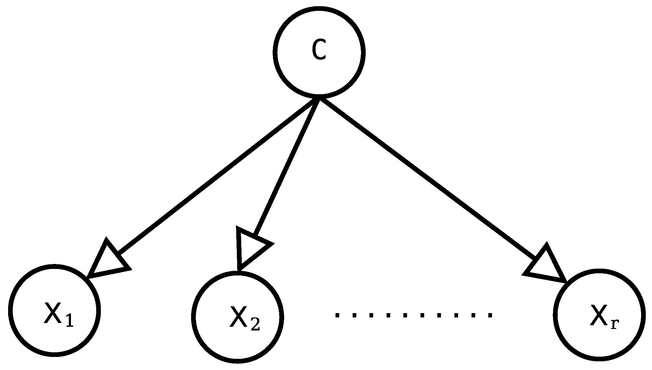
Let $\mathcal{D}$ be a dataset, with size N, and with values in a set $\mathcal{L}$ of (discrete or discretized) attribute variables $\left\{X_i|i=1,\dots ,r\right\}$, where each variable has a set of possible states or cases ${\mathrm{\Omega }}_{X_i}=\{x_1^i,x_2^i,\dots ,x_{|{\mathrm{\Omega }}_{X_i}|}^i\}$, and a class variable C, whose states are ${\mathrm{\Omega }}_C=\{c_1,c_2,\dots ,c_k\}$. The objective is to obtain information from the dataset in such a way that, given an observation (a set of values of all the attribute variables), it is possible to associate this with a value of the class variable.

If we represent the new sample as $\mathbf{x}$, with $\mathbf{x}=\{x_{h_1}^1,..,x_{h_r}^r\}$. The Naive Bayes (Figure 1) predicts value $c_m$ of C in the following way:

$$c_m=arg\underset{c_j}{max}\left(p\left(c_j\right|\mathbf{x})\right),$$

with $p\left(c_j\right|\mathbf{x})$ the probability of each $c_j$ in the subset of the training set determined by $\mathbf{x}$ (subset of the sample that verifies that $X_i=x_{h_i}^i,\forall i$).

Now, based on the assumption that the attribute variables are independent given the class variable, the predicted value can be expressed as

$$c_m=arg\underset{c_j}{max}\left(p\left(c_j\right)\prod _{i=1}^{r}p(x_{h_i}^i|c_j)\right).$$

The key to success of the Naive Bayes is its simplicity: no Bayesian network structure learning algorithm is required because its structure is fixed, the parameters of the model need only be estimated from the dataset using only bi-dimensional statistics for the class and each attribute and, as we have seen, the classification process is very efficient.

The Naive Bayes model shows remarkable results in accuracy, taking into account its clearly unrealistic assumptions: first, each attribute is conditionally independent from the other attributes given the class and, second, all of the variables have the same influence on the class. These assumptions can also cause some problems: the influence on the class of two highly correlated attributes may be overamplified by the model or a really irrelevant variable may only add noise to the classification. In any case, the solution may be to remove some attributes by using variable selection. The exhaustive search in the space of all of the variables combinations for the Naive Bayes requires the computation of $2^r$ structures, which is often prohibitive.

4. Variable Selection Methods

The aim of a variable selection method is to select a subset of variables that can effectively replace the original set of attributes while reducing the unfavourable effects of irrelevant or redundant features and still provide good results or, even better, improve the model performance.

Taking into account that many data mining techniques were originally not designed to work with considerable amounts of irrelevant/redundant features, such as the Naive Bayes classifier, the variable extraction is almost a requisite to work with many datasets. Furthermore, the variable selection stage will allow us to work efficiently with large datasets. Nevertheless, we must bear in mind that variable extraction adds an extra level of complexity to the process and there is no guarantee that the optimal subset of variables will be selected.

The methods to select variables depends on whether a base classifier is used as reference or not. They are generally grouped into two classes: (i) filter methods: select variables independently in relation to the classification method used; and (ii) wrapper methods: depend on the classification method subsequently used (Hall and Holmes [1]).

The wrapper methods need to check many steps subsets of variables in the base classifier. This procedure makes them few suitable when the amount of features is huge. When the amount of data increases, the filter methods are more appropriate. Although the use of a determinate filter method depends on its computational cost, it may not be possible to be use due to the big size of data or number of features.

The most popular filter methods applied on the Naive Bayes classifier use as a tool the mutual information measure of each attribute and the class variable [20], which is just the same procedure as the one of the information gain. A filter method that evaluates subsets of features also can have a a high computational cost, but normally lower than the ones of the wrapper methods when they are used to improve the Naive Bayes.

4.1. Info-Gain

This metric was introduced by Quinlan as the basis for his ID3 model [2]. This model has the following main features: it was defined to obtain decision trees with discrete variables, it does not work with missing values, a pruning process is not carried out, and it is based on Shannon’s entropy [4]. This split criterion can therefore be defined on an attribute variable X given the class variable C in the following way:

$$IG(X,C)=S\left(C\right)-S\left(C\right|X),$$

where $S\left(C\right)$ is the entropy of C: $S\left(C\right)=-{\sum }_{j}p\left(c_j\right)logp\left(c_j\right),$ with $p\left(c_j\right)=p(C=c_j)$, the probability of each value of the class variable estimated in the training dataset. In the same way,

$$S\left(C\right|X)=-\sum _t\sum _{j}p\left(c_j\right|x_t)logp\left(c_j\right|x_t),$$

where $x_t,t=1,..,\left|{\mathrm{\Omega }}_X\right|$, is each possible state of X and $c_j,j=1,..,k$, each possible state of C. Finally, we can obtain the following reduced expression for the Info-Gain criterion:

$$IG(X,C)=\sum _t\sum _{j}p(c_j,x_t)log\frac{p(c_j,x_t)}{p\left(c_j\right)p\left(x_t\right)}.$$

This criterion is also known as the Mutual Information Criterion and it is widely used for measuring the dependence degree between an attribute variable and the class variable. It tends to select attribute variables with many states and consequently results in excessive ramification.

The IG criterion can be used as a variable selection method. It creates a rank of informative variables. It principal drawback is that it always gives a non-negative value of gain in information:

$$IG(X,C)\ge 0,\forall X.$$

This result is a direct consequence of the Gibb’s inequality on two probability distributions $p=\left(p_i\right)$ and $q=\left(q_i\right)$ on a finite set X:

$$-\sum _i{p}_{i}log{p}_i\le \sum _i{p}_{i}log{q}_i.$$

In the case of the $IIG$, it can be considered the probability distribution q on $C\times X$ defined as $q(c_j,x_t)=p\left(c_j\right)p\left(x_t\right)$, where p is the above probability distribution based on the frequencies in the dataset.

As that value is always non-negative, the IG criterion creates a rank of features based on each gain in information. The problem is where to fix the threshold to use as filter to select the variables. The maximum gain in information is $log\left|C\right|$. Then, the function to consider as threshold must be $\alpha log\left|C\right|$, with $\alpha \in [0,1]$.

4.2. Imprecise Info-Gain

The Imprecise Info-Gain criterion was first used for building decision trees in Abellán and Moral’s method [10]. In a similar way to ID3, this tree is only defined for discrete variables; it cannot work with missing values; and it does not carry out a posterior pruning process. It is based on the application of uncertainty measures on convex sets of probability distributions. More specifically, probability intervals are extracted from the dataset for each case of the class variable using Walley’s imprecise Dirichlet model [12] (IDM), which represents a specific kind of convex set of probability distributions, and on these the maximum entropy is estimated.

As we explained in previous sections, the IDM depends on a parameter s and it estimates that (in a given dataset) the probabilities for each value of the class variable ($c_j$) are within the interval:

$$p\left(c_j\right)\in \left[\frac{n_{c_j}}{N+s},\frac{n_{c_j}+s}{N+s}\right],$$

with $n_{c_j}$ as the frequency of the set of values $(C=c_j)$ in the dataset.

If we label $K\left(C\right)$ and $K\left(C\left|\right(X=x_t)\right)$ for the following sets of probability distributions q on ${\mathrm{\Omega }}_C$:

$$K\left(C\right)=\left\{q|q\left(c_j\right)\in \left[\frac{n_{c_j}}{N+s},\frac{n_{c_j}+s}{N+s}\right]\right\},$$

$$K\left(C\left|\right(X=x_t)\right)=\left\{q|q\left(c_j\right)\in \left[\frac{n_{\{c_j,x_t\}}}{N+s},\frac{n_{\{c_j,x_t\}}+s}{N+s}\right]\right\},$$

with $n_{\{c_j,x_t\}}$ as the frequency of the set of values $(C=c_j,X=x_t)$ in the dataset, we can define the Imprecise Info-Gain for each attribute variable X as:

$$IIG(X,C)=S^{*}\left(K\left(C\right)\right)-\sum _{t}p\left(x_t\right)S^{*}\left(K\left(C\left|\right(X=x_t)\right)\right),$$

where $S^{*}\left(\right)$ is the maximum entropy function of a credal set.

For the previously defined intervals and for a value of $s=1$, Abellán’s procedure [21] has a low computation cost. This value is the one recommended by Walley [12] and the one used to build decision trees in Abellán and Moral [10]. Given a credal set $K\left(C\right)$ defined as above, we must first determine the set $B=\left\{c_j\right|n_{c_j}={\min }_i\left\{n_{c_i}\right\}\}$. Let $\left|B\right|$ be the cardinal of the set B. If we use $\widehat{p}$ to denote the distribution where the maximum of entropy will be reached, the procedure of Abellán [21] for $s=1$ can be expressed in the following way:

$$\widehat{p}\left(c_i\right)=\left\{\begin{array}{c}\frac{n_{c_i}}{N+s}{c}_i\notin B,\hfill \\ \frac{n_{c_i}+s/\left|H\right|}{N+s}{c}_i\in B.\hfill \end{array}\right.$$

In this procedure, we split the value of s as uniformly as it is possible between the states of C with lower frequency. For values $s>1,$ the algorithm to find the maximum entropy value has more computational cost.

In Abellán, Klir and Moral [6], we can see that the function of the maximum entropy includes two kinds of uncertainty: conflict and non-specificity. The first one is somewhat similar to the one in PT, well quantified by the Shannon’s entropy. The second one is a new type of uncertainty that does not appear in PT.

The maximum of entropy is the only measure that verifies a similar set of important properties on credal sets rather than the classic entropy in PT (see Abellán et al. [6]). The use of the maximum entropy function on this type of sets is also justified with the following sentences of Jaynes [22] about the sense of this measure:

“The fact that a certain probability distribution maximizes entropy subject to certain constraints representing our incomplete information, is the fundamental property which justifies use of that distribution for inference, it agrees with everything that is known, but carefully avoids assuming anything that is not known.”

The practical application of the IIG procedure can be easily explained without the concept of credal set, using only the frequencies $n_{c_j}$ and the expression of the $\widehat{p}$ values. Let us apply the following notation:

• $n=(n_{c_1},\cdots ,n_{c_k});$
• $n^{\prime }$ is the array n where the mass $s=1$ is shared among the minimum values (as in $\widehat{p}$);
• $S\left(n\right)=S\left(C\right)$ is the entropy using a notation on non-normalized values;
• $S\left(n^{\prime }\right)$ is the maximum entropy value of C. It is a consequence of the above points;
• $n_{X=x_t}$ is the array $(n_{\{c_1,x_t\}},\cdots ,n_{\{c_k,x_t\}}).$

With the above notation, IIG can be expressed as follows:

$$IIG(C,X)=S\left(n^{\prime }\right)-\sum _{X=x_t}p(X=x_t)S(n_{X=x_t}^{\prime }).$$

The original procedure to build decision trees [10], where the IIG was presented, uses the feature with the highest value of IIG to be inserted in a node.

4.3. IG versus IIG

One of the most significative differences between the IG and the IIG criteria is that the IIG can be negative. This situation never occurs with the IG criterion. This important characteristic allows the IIG criterion to discard variables that worsen the information on the class variable. This property allows us to detect directly which features are irrelevant as they will obtain negative values of information gain, which is equivalent to a waste of information.

With the IG criterion, we obtain a feature ranking, but this does not give a subset of variables, so we must decide which variables must be selected. To address this issue, the variables to be selected must have an IG value greater than or equal to a threshold. The threshold used depends on an $\alpha$ parameter and the number of states of the class variable for each dataset, hence we have that

$$threshold=\alpha \times log\left(k\right),$$

where $\alpha \in [0,1]$ and $k=\left|C\right|$.

In the Example 1, we can see a practical case where the difference between both criteria can be appreciated. In that example, we can see that some features can be selected by the IG criterion but not selected by the IIG.

Example 1.

Let C be a class variable with two possible states $\{c_1,c_2\}$. We consider that we have the following frequencies $\{c_1:9,c_2:4\}$. We also consider that we only have two attribute variables $X_1,X_2$, with possible values $X_1\in \{x_1^1,x_2^1\}$, and $X_2\in \{x_1^2,x_2^2,x_3^2\}$. The frequencies of each combination of states are the following ones:

$$\begin{array}{cc}{X}_1=x_1^1\to & (5 of class c_1, 3 of class c_2),\\ X_1=x_2^1\to & (4 of class c_1, 1 of class c_2),\\ X_2=x_1^2\to & (2 of class c_1, 2 of class c_2),\\ X_2=x_2^2\to & (5 of class c_1, 2 of class c_2),\\ X_2=x_3^2\to & (2 of class c_1, 0 of class c_2).\end{array}$$

Considering the IG criterion, we always have an improvement in the gain of information. The values obtained with this criterion are the following ones (using the natural logarithm):

$$IG(C,X_1)=0.6172-\frac{8}{13}0.6615-\frac{5}{13}0.5004=0.0177,$$

$$IG(C,X_2)=0.6172-\frac{4}{13}0.6931-\frac{7}{13}0.5983-\frac{2}{13}0=0.0818.$$

Here, the feature $X_2$ produces the greater gain of information by the IG criterion. Now, if we set $\alpha =0.1$, then $threshold=0.0301$, and only $X_2$ would be selected. If we set $\alpha =0.01$, then $threshold=0.003$, and both features would be selected.

However, with the IIG criterion (and $s=1$), we have the following values:

$$IIG(C,X_1)=0.6518-\frac{8}{13}0.6850-\frac{5}{13}0.6368=-0.0002,$$

$$IIG(C,X_2)=0.6518-\frac{4}{13}0.6931-\frac{7}{13}0.6615-\frac{2}{13}0.6368=-0.0157.$$

Now, none of the variables would be selected by the IIG criterion.

The different results obtained in the above example are motivated by the use of the maximum entropy measure. The best value for the $\alpha$ parameter to obtain the best set of informative features with the IG criterion is an open question. In that example, we can see that different values of that parameter $\alpha$ produce a different set of selected variables.

To show that the both criteria perform differently, in a contrary situation to the one expressed by the Example 1, we can see the following example based on a real dataset.

Example 2.

We consider the dataset anneal from the University of California Irvine (UCI) repository of machine learning datasets [23] that we will use in our experimentation in the next sections. This dataset has 38 features and its class variable has six states ($k=6$). The gain in information of the last 12 features (the worse ones) for both criteria are presented in

Table 1. Gain in information for the 12 worse features in anneal dataset using the IG and IIG criteria.

IG	Feature	IIG	Feature
0.0193	bore	0.0118	exptl
0.0182	lustre	0.0087	lustre
0.0156	exptl	0.0044	bore
0.0039	packing	0	product-type
0.0004	bc	0	jurofm
0	product-type	0	p
0	jurofm	0	s
0	p	0	m
0	s	0	corr
0	m	0	marvi
0	corr	−0.0019	bc
0	marvi	−0.0052	packing

. The values are obtained using the same procedure as the one in Example 1.

Considering that $log\left(6\right)=1.7917$, the threshold for $\alpha =0.01$ is $0.0179$. Hence, the IG criterion with that value of α does not select the features from the “exptl” feature to the bottom, including that feature. Observing the value of gain of information using the IIG criterion for that feature, we see that this feature is selected by the IIG criterion because it has a positive value ($0.0118$).

The above example expresses a situation where a feature is selected by the IIG criterion but not for the IG criterion with its less restrictive $\alpha$ value. Then, that feature is also not selected using the rest of $\alpha$ values.

5. Experimentation

In this section, we shall describe the experiments carried out and show the results obtained. For our purpose, we have used a wide and different set of 30 known datasets, obtained from the UCI repository of machine learning datasets [23]. A brief description of these can be found in

Table 2. Datasets used in the experimentation.

Dataset	N	Attrib	Num	Nom	k
anneal	898	38	6	32	6
arrhythmia	452	279	206	73	16
audiology	226	69	0	69	24
autos	205	25	15	10	7
breast-cancer	286	9	0	9	2
cmc	1473	9	2	7	2
colic	368	22	7	15	2
credit-german	1000	20	7	13	2
diabetes	768	8	8	0	2
glass-2	163	9	9	0	2
hepatitis	155	19	4	15	2
hypothyroid	3772	29	7	22	4
ionosphere	351	35	35	0	2
japanese	690	15	9	6	2
kr-vs-kp	3196	36	0	36	2
madelon	2600	500	500	0	2
mushroom	8123	22	0	22	2
musk1	476	166	166	0	2
musk2	6598	166	166	0	2
semeion	1593	156	256	0	10
segment	2310	19	19	0	7
spectrometer	531	131	130	1	48
sick	3772	29	7	22	2
solar-flare	323	12	0	12	2
sonar	208	60	60	0	2
soybean	683	35	0	35	19
sponge	76	44	0	44	3
vote	435	16	0	16	2
vowel	990	12	10	2	11
zoo	101	16	1	15	7

, where column “N” is the number of instances in the datasets, column “Attrib” is the number of attribute variables, column “Num” is the number of numerical variables, column “Nom” is the number of nominal variables, and column “k” is the number of cases or states of the class variable (always a nominal variable).

The Weka software (ver. 3.8) [24] has been used for the experimentation. The procedure of selecting attributes with the IIG method was implemented using data structures of Weka and the IDM parameter was set to $s=1$, i.e., the value used in the original methods of [18]. The reasons to use this value were: first, it was the value recommended by Walley [12]; and, second, the procedure to obtain the maximum entropy value reaches its lowest computational cost for this value [21].

As we have seen above, the IIG criterion allows us to discard those variables with negative information gain, while the IG measure only obtains a attribute ranking, which means that a threshold must be chosen to discard those irrelevant features. The selected threshold is determined by the number of states of the class variable and a parameter $\alpha$. For our experiments, we have chosen four different values For values lower than $0.01$, the IG criterion selects all of the features for many of the datasets; and for values higher than $0.1$, the criterion selects a very low number of features and then the performance of the Naive Bayes is very poor—for that parameter: $0.01$, $0.02$, $0.05$ and $0.1$.

In the experimentation, for each dataset, we applied the following procedure of 10-fold-cross validation repeated 10 times: the dataset is separated into 10 subsets, each one is used as a test set and the set obtained joining the other nine subsets are used as a training set. Thus, we have 10 training sets and 10 test sets. This procedure is repeated 10 times with a previous random reordering. Finally, it produces 100 training sets and 100 test sets. Using only the training set, features are selected via the IG and IIG methods obtaining a final subset of features. The Naive Bayes classifier is built on that subset, and the same subset of features is used for the test. Finally, Naive Bayes is applied on the test set. These results are compared with the Naive Bayes classifier with no variable selection scheme following the same validation procedure.

In summary, we have tested the Naive Bayes classifier without a variable selection and Naive Bayes with a previous variable selection procedure, using the IIG criterion and the IG criterion (this last one with four different thresholds).

The percentages of correct classifications for each dataset and each method, are presented in

Table 3. Percentages of the average Accuracy and Standard Deviations of the Naive Bayes classifier considering all of the methods of variable selection on each dataset.

Dataset	$\mathit{NB}$	${\mathit{IG}}_{0.01}$	${\mathit{IG}}_{0.02}$	${\mathit{IG}}_{0.05}$	${\mathit{IG}}_{0.1}$	$\mathit{IIG}$
anneal	86.59 ± 3.31	86.16 ± 3.42	86.20 ± 3.38	86.36 ± 3.07	90.12 ± 3.14	86.47 ± 3.39
arrhythmia	62.40 ± 6.97	66.66 ± 5.90	66.49 ± 5.96	62.14 ± 6.12	54.29 ± 1.21	67.06 ± 5.79
audiology	72.64 ± 6.10	73.60 ± 6.19	74.08 ± 6.99	66.97 ± 7.09	68.30 ± 7.98	74.27 ± 5.79
autos	57.41 ± 10.77	57.45 ± 11.15	56.53 ± 11.40	57.40 ± 11.45	60.90 ± 11.63	57.45 ± 11.15
breast-cancer	72.70 ± 7.74	72.79 ± 7.93	73.01 ± 7.99	71.31 ± 7.21	70.30 ± 1.37	72.76 ± 7.98
cmc	50.48 ± 4.22	50.36 ± 4.24	50.41 ± 4.48	47.69 ± 3.43	42.70 ± 0.25	50.48 ± 4.22
horse-colic	78.70 ± 6.20	78.78 ± 5.72	80.08 ± 5.69	82.32 ± 5.81	80.33 ± 5.88	78.65 ± 5.77
credit-german	75.16 ± 3.48	74.55 ± 4.06	74.14 ± 3.60	68.79 ± 2.81	69.50 ± 2.04	75.21 ± 3.68
diabetes	75.75 ± 5.32	75.09 ± 5.52	74.99 ± 5.51	75.70 ± 5.54	74.62 ± 4.96	75.09 ± 5.52
glass2	62.43 ± 8.86	64.05 ± 9.05	64.05 ± 9.05	64.05 ± 9.05	64.89 ± 10.13	64.05 ± 9.05
hepatitis	83.81 ± 9.70	85.09 ± 9.48	84.96 ± 9.92	84.69 ± 9.24	82.15 ± 8.88	84.38 ± 9.88
hypothyroid	95.30 ± 0.73	94.80 ± 0.81	94.78 ± 0.80	94.80 ± 0.78	93.97 ± 0.86	95.29 ± 0.76
ionosphere	82.17 ± 6.14	82.42 ± 6.23	82.42 ± 6.23	82.45 ± 6.20	82.48 ± 6.16	82.42 ± 6.23
japanese	77.86 ± 4.18	77.90 ± 4.23	77.84 ± 4.22	77.01 ± 4.25	76.83 ± 4.63	77.99 ± 4.29
kr-vs-kp	87.79 ± 1.91	89.09 ± 2.09	89.40 ± 1.92	90.43 ± 1.51	80.29 ± 7.23	87.80 ± 1.92
madelon	59.44 ± 2.66	60.58 ± 3.05	60.34 ± 2.97	52.97 ± 4.51	50.00 ± 0.00	59.54 ± 3.09
mushroom	95.76 ± 0.73	95.60 ± 0.80	95.57 ± 0.79	95.85 ± 0.81	95.72 ± 0.78	95.76 ± 0.73
musk1	73.99 ± 8.04	74.62 ± 7.74	74.62 ± 7.74	73.38 ± 7.67	70.40 ± 6.22	74.62 ± 7.74
musk2	83.91 ± 1.62	83.89 ± 1.62	83.44 ± 1.54	82.47 ± 1.55	82.52 ± 1.66	83.91 ± 1.62
segment	80.17 ± 2.12	79.92 ± 1.90	79.92 ± 1.89	78.97 ± 1.95	78.97 ± 1.95	80.17 ± 2.12
semeion	86.36 ± 2.70	86.43 ± 2.59	86.33 ± 2.71	80.75 ± 2.79	41.07 ± 3.00	86.43 ± 2.59
sick	92.75 ± 1.36	94.59 ± 1.24	95.02 ± 1.10	96.61 ± 0.80	93.88 ± 0.08	93.79 ± 1.36
solar-flare1	93.02 ± 4.29	94.81 ± 3.78	96.14 ± 2.70	97.84 ± 1.42	97.84 ± 1.42	97.56± 1.92
sonar	67.71 ± 8.66	66.42 ± 9.47	66.42 ± 9.47	66.42 ± 9.47	67.22 ± 10.72	66.42 ± 9.47
soybean	92.94 ± 2.92	92.94 ± 2.92	92.65 ± 2.88	92.68 ± 2.88	87.73 ± 3.33	92.94 ± 2.92
spectrometer	42.06 ± 5.99	42.70 ± 5.80	42.70 ± 5.80	42.70 ± 5.80	41.92 ± 5.53	42.70 ± 5.80
sponge	92.11 ± 9.16	89.79 ± 10.83	89.09 ± 10.79	92.75 ± 9.63	94.75 ± 6.45	93.64 ± 7.32
vote	90.02 ± 3.91	90.00 ± 4.11	90.00 ± 4.11	90.02 ± 4.11	89.93 ± 4.13	90.02 ± 3.95
vowel	66.79 ± 4.36	67.45 ± 4.70	67.42 ± 4.51	64.81 ± 5.11	58.49 ± 5.08	67.11 ± 4.54
zoo	95.07 ± 5.86	95.07 ± 5.86	95.07 ± 5.86	95.16 ± 5.86	95.06 ± 5.87	95.07 ± 5.86
Average	77.78 ± 5.0	78.12 ± 5.08	78.14 ± 5.07	77.18 ± 4.93	74.57 ± 4.42	78.30 ± 4.88

with the standard deviation to appreciate the variation of each iteration of the methods.

Table 4. Average number of selected attributes for the methods of variable selection on each dataset.

Dataset	${\mathit{IG}}_{0.01}$	${\mathit{IG}}_{0.02}$	${\mathit{IG}}_{0.05}$	${\mathit{IG}}_{0.1}$	$\mathit{IIG}$
anneal	23.74	13.17	10.84	6.00	29.00
arrhythmia	76.15	72.21	17.18	0.03	118.06
audiology	34.70	20.63	11.22	8.14	55.26
autos	22.50	20.45	19.05	11.60	22.51
breast-cancer	6.13	4.93	3.50	0.00	5.46
cmc	6.52	4.96	1.02	0.00	9.00
horse-colic	15.73	12.98	7.91	2.16	16.76
german-credit	9.74	5.48	1.02	0.12	14.20
diabetes	7.06	6.22	4.11	1.02	7.06
glass2	4.97	4.97	4.97	3.62	4.97
hepatitis	13.70	11.80	9.54	3.91	12.93
hypothyroid	4.00	3.42	3.00	1.00	8.64
ionosphere	32.42	32.42	32.35	32.10	32.42
japanese	12.20	11.61	6.79	5.89	14.17
kr-vs-kp	13.92	7.05	3.00	2.35	33.07
madelon	9.25	7.37	0.33	0.00	17.60
mushroom	20.00	19.00	13.15	12.69	21.00
musk1	134.43	134.43	85.54	16.83	134.43
musk2	165.14	161.60	144.24	81.82	166.00
segment	16.16	16.00	15.00	15.00	18.00
semeion	251.69	222.25	87.99	7.47	251.69
sick	6.00	4.03	2.00	1.00	14.80
solar-flare1	5.92	3.62	0.00	0.00	1.02
sonar	21.14	21.14	21.14	8.09	21.14
soybean	34.94	30.78	27.81	15.64	35.00
spectrometer	93.99	93.99	93.99	86.16	93.99
sponge	34.18	29.90	11.30	3.78	4.68
vowel	9.38	9.00	6.22	3.36	10.38
vote	14.00	14.00	13.73	12.50	14.99
zoo	16.00	15.47	13.60	12.89	15.71
Average	37.19	33.83	22.38	11.84	40.13

presents the average number of attributes selected for each method of variable selection. In addition, the average times in seconds consumed for each method, when they are applied on a pair of Training and Test sets, are shown in

Table 5. Average time in seconds for each method when it is applied on a pair of Training and Test sets.

NB	${\mathit{IG}}_{0.01}$	${\mathit{IG}}_{0.02}$	${\mathit{IG}}_{0.05}$	${\mathit{IG}}_{0.1}$	$\mathit{IIG}$
0.013	0.039	0.038	0.037	0.035	0.046

.

We have compared the results of the Naive Bayes classifier joint with a previous variable selection method with the ones of the original classifier without a previous procedure for variable selection. Following the recommendation of Demšar [25], we have used the known Wilcoxon Signed-Ranks test [26] for the pairwise comparisons. We have considered that this comparative is more appropriate than the one of comparing all the methods joined because four of them are the same method varying the value of the threshold, and the principal aim is the improvement of the Naive Bayes classifier. We have carried out the tests using the $Keel$ software (ver. 2015-03-23) [27].

The Wilcoxon Signed-Ranks test [26] is a non-parametric test that ranks the differences in performance of two classifiers of each dataset comparing the ranks for the positive and the negative differences. It takes into account the commensurability of the differences that the Sign Test does not [25]. It is used to compare two related samples, matched samples, or repeated measurements on a single sample to check whether their population mean ranks differently.

Given $A_1$ and $A_2,$ two paired sets of data with a sample size of N:

$$A_1=\{A_{11},\cdots ,A_{1N}\},$$

$$A_2=\{A_{21},\cdots ,A_{2N}\}.$$

The null hypothesis is that the samples mean are equivalent, and the test is based on the following statistic:

$$W=\sum _{i=1}^{N^{\prime }}\left[sing(A_{1i}-A_{2i})Ran{k}_i\right],$$

where $N^{\prime }$ is the sample size without ties; $sing$ is the function that returns the sing of a value; and $Ran{k}_i$ is the ranking associated with the order established by the values of the set $\left\{\right|A_{1i}-A_{2i}|,i=1,\cdots ,N^{\prime }\}$. W follows a distribution with an expected value of 0 and a variance of $\frac{N^{\prime }(N^{\prime }+1)(2N^{\prime }+1)}{6}.$

In

Table 6. Wilcoxon’s test about the accuracy of the algorithms. We use the symbol ○ if the method in the column significantly improves the algorithm in the row and the symbol ● expresses that the method in the row improves significantly the method in the column. The cells’ upper diagonal have a significance level of $0.90$ and the lower ones have a significance level of $0.95$.

Algorithm	$\mathit{NB}$	${\mathit{IG}}_{0.01}$	${\mathit{IG}}_{0.02}$	${\mathit{IG}}_{0.05}$	${\mathit{IG}}_{0.1}$	$\mathit{IIG}$
$NB$	-				●	○
$I{G}_{0.01}$		-			●
$I{G}_{0.02}$			-		●
$I{G}_{0.05}$				-	●	○
$I{G}_{0.1}$	○	○	○	○	-	○
$IIG$	●			●	●	-

, we compare each method with the others using the Wilcoxon test.

Comments on the Results

Table 3 shows that the predictive accuracy of the Naive Bayes classifier usually improves when a variable selection step is carried out. However, it should be noted that better results are not always achieved. After surveying the accuracy results, it becomes clear that, for the case of $I{G}_{0.05}$ and $I{G}_{0.1},$ the results are worse. If we take a closer look, the best overall results are achieved using the IIG criterion. Henceforth, we can state that, in general, the Naive Bayes classifier offers better performance in predictive accuracy when the IIG criterion is used as a previous variable selection step.

Regarding accuracy, we must note that the IIG criterion does not always achieve the best performance. Depending on the dataset and the threshold used, the IG measure with different thresholds can return the best results in some cases. Therefore, the performance of the IG criterion can be improved by carrying out a search or study to determine the most appropriate threshold for every dataset. However, it is still an open problem: how to select the correct threshold value depending on the properties of each dataset. On the other hand, a study to determine the best threshold for each problem can add more complexity to the variable selection step.

With respect to the results about the number of selected features, shown in Table 4, we should mention that the variable selection performed using the IIG criterion is less aggressive than the different options based on the IG measure that were evaluated. The fact that the IIG does not require a threshold, since it removes variables with a negative information gain, may suggest that this criterion only discards those features that are truly irrelevant and add no information about the class variable. This table also shows the problem of using a threshold for the IG criterion. We can observe that, for the same value of the $\alpha$ parameter, the number of selected variables varies notably. It is clear that the greater the value of the $\alpha$ parameter, the lower will be the number of chosen variables for the same dataset. It can be seen that, for some datasets and using $\alpha =0.01$, the number of variables selected is very similar to the number obtained using the IIG criterion. Then, for those datasets, the differences in performance are due to the different treatment of the information from both methods, as was shown in Example 1. In other datasets and using $\alpha =0.1$, the IG measure does not select any variable.

It is important to remark that we found performance differences when comparing two procedures that select a similar average number of variables, i.e., IG${}_{0.01}$ and IIG. For some datasets (e.g., audiology and german-credit), the first procedure selects a notably lower number of variables than the second one; for other datasets (e.g., solarflare and sponge), the first one selects a notably higher number of variables than the second one. However, in all these cases, the performance in accuracy of the IIG criterion is significantly better; and the IIG criterion is clearly more informative for variable selection.

The accuracy results in Table 3 show that Naive Bayes is usually better combined with the IIG criterion used in a previous feature selection step. Using the IIG, the results never deteriorate significantly. We cannot say the same for the IG with different threshold levels. For example, if we compare the results of percentage of accuracy for IG with $\alpha =0.05$ and the results using the original NB, we get the following results of clear improvement or deterioration (IG${}_{0.05}|$NB):

$$horsecolic⟶82.32|78.70,$$

$$german-credit⟶75.16|68.79.$$

The difference can be close to $7\%$. With $\alpha =0.01$, we get similar results, such as these (IG${}_{0.01}|$NB):

$$hepatitis⟶85.09|83.81,$$

$$sponge⟶89.79|92.11.$$

Table 5 shows that all the procedures have an extremely low computational cost, with average processing time below a tenth of a second. Another outcome is that Naive Bayes is the fastest method (as expected, since it has no variable selection stage). The different versions of the IG achieve improved response times depending on the number of variables selected. The IIG approach, though very fast, is slower than the rest of the approaches studied, as working with imprecise probabilities and the maximum entropy measure has a greater computational cost than precise probabilities and the Shannon entropy.

The statistical differences are analyzed via the Wilcoxon test carried out between each pair of methods. The results are presented in Table 6. Now, only the IIG approach achieves better results than Naive Bayes without variable selection, and these results are statistically significant for each level of significance used. None of the IG variants studied produce significantly better results than the Naive Bayes classifier without variable selection. We also note that IG with $\alpha =0.1$ is notably worse than the rest of the proposals.

6. Conclusions

As was pointed out in previous sections, variable selection is an important step in the preprocessing stage for data mining. In this paper, we have presented a new method to select variables based on imprecise probabilities and the maximum entropy measure to improve a very known classification method. We have shown, via an experimental study, that the predictive accuracy of the Naive Bayes classifier improves with the new variable selection method. Using an important statistical test, we obtain that the differences are statistically significant in favour of the use of the new method.

We compared the new method with a similar classical method based on precise entropy, called Info-Gain (IG). It must be remarked that in the same test carried out to compare the original Naive Bayes with the one using IG as a previous variable selection, we do not obtain significant statistical differences.

An important difference of the new method with respect to the classical one used for comparison is that the IG requires using a threshold to perform variable selection. Choosing the best threshold for each dataset is a difficult task. It should be emphasized that our proposal does not require setting a threshold, since variables with a negative information gain are discarded. The new method provides a quick and improved procedure for the preliminary step of variable selection for the Naive Bayes classifier that outperforms the IG approach, while removing the requirement of setting a threshold. The results presented in this work reinforce this assertion.

The final conclusion of this work is that the combination of the new variable selection method presented here with the Naive Bayes classifier provides an extremely useful tool for datasets with a very large number of features and a huge amount of data, where using complex methods is not computationally feasible. This is one of our tasks for future work.

A more immediate task for future work is to explore the use of the IIG criterion in complex methods to select variables based on IG. We think that this could provide an interesting improvement.

References

- Hall, M.A.; Holmes, G. Benchmarking attribute selection techniques for discrete class data mining. IEEE Trans. Knowl. Data Eng. 2003, 15, 1437–1447. [Google Scholar] [CrossRef]
- Quinlan, J.R. Induction of Decision Trees. Mach. Learn. 1986, 1, 81–106. [Google Scholar] [CrossRef]
- Walley, P. Statistical Reasoning with Imprecise Probabilities; Taylor & Francis: London, UK, 1991. [Google Scholar]
- Shannon, C.E. A Mathematical Theory of Communication. Bell Syst. Tech. J. 1948, 27, 379–423. [Google Scholar] [CrossRef]
- Klir, G.J. Uncertainty and Information: Foundations of Generalized Information Theory; John Wiley & Sons: Hoboken, NJ, USA; New York, NY, USA, 2005. [Google Scholar]
- Abellán, J.; Klir, G.; Moral, S. Disaggregated total uncertainty measure for credal sets. Int. J. Gen. Syst. 2006, 35, 29–44. [Google Scholar] [CrossRef]
- Abellán, J.; Masegosa, A. Requirements for total uncertainty measures in Dempster-Shafer theory of evidence. Int. J. Gen. Syst. 2008, 37, 733–747. [Google Scholar] [CrossRef]
- Abellán, J.; Bossé, É. Drawbacks of Uncertainty Measures Based on the Pignistic Transformation. IEEE Trans. Syst. Man Cybern. 2016, 1–7. [Google Scholar] [CrossRef]
- Mantas, C.J.; Abellán, J. Analysis and extension of decision trees based on imprecise probabilities: Application on noisy data. Expert Syst. Appl. 2014, 41, 2514–2525. [Google Scholar] [CrossRef]
- Abellán, J.; Moral, S. Building classification trees using the total uncertainty criterion. Int. J. Intell. Syst. 2003, 18, 1215–1225. [Google Scholar] [CrossRef]
- De Campos, L.M.; Huete, J.F.; Moral, S. Probability intervals: A tool for uncertain reasoning. Int. J. Uncertain. Fuzziness Knowl. Based Syst. 1994, 2, 167–196. [Google Scholar] [CrossRef]
- Walley, P. Inferences from multinomial data: Learning about a bag of marbles (with discussion). J. R. Stat. Soc. Ser. B Methodol. 1996, 58, 3–57. [Google Scholar]
- Dempster, A.P. Upper and Lower Probabilities Induced by a Multivalued Mapping. Ann. Math. Stat. 1967, 38, 325–339. [Google Scholar] [CrossRef]
- Shafer, G. A Mathematical Theory of Evidence; Princeton University Press: Princeton, NJ, USA, 1976. [Google Scholar]
- Klir, G.J.; Smith, R.M. On Measuring Uncertainty and Uncertainty-Based Information: Recent Developments. Ann. Math. Artif. Intell. 2001, 32, 5–33. [Google Scholar] [CrossRef]
- Abellán, J.; Moral, S. An algorithm to compute the upper entropy for order-2 capacieties. Int. J. Uncertain. Fuzziness Knowl. Based Syst. 2006, 14, 141–154. [Google Scholar] [CrossRef]
- Klir, G.; Wierman, M. Uncertainty-Based Information: Elements of Generalized Information Theory; Springer Science & Business Media: Berlin, Germany, 1999. [Google Scholar]
- Abellán, J.; Moral, S. Upper entropy of credal sets. Applications to credal classification. Int. J. Approx. Reason. 2005, 39, 235–255. [Google Scholar] [CrossRef]
- Duda, R.O.; Hart, P.E. Pattern Classification and Scene Analysis; John Wiley & Sons: New York, NY, USA, 1973. [Google Scholar]
- Pazzani, M.; Billsus, D. Learning and Revising User Profiles: The Identification of Interesting Web Sites. Mach. Learn. 1997, 27, 313–331. [Google Scholar] [CrossRef]
- Abellán, J. Uncertainty measures on probability intervals from the imprecise Dirichlet model. Int. J. Gen. Syst. 2006, 35, 509–528. [Google Scholar] [CrossRef]
- Jaynes, E.T. Notes on Present Status and Future Prospects. In Maximum Entropy and Bayesian Methods; Springer: Dordrecht, The Netherlands, 1990; pp. 1–13. [Google Scholar]
- Lichman, M. UCI Machine Learning Repository. 2013. Available online: http://archive.ics.uci.edu/ml/ (accessed on 24 May 2017).
- Witten, I.H.; Frank, E.; Hall, M.A.; Pal, C.J. Data Mining: Practical Machine Learning Tools and Techniques; Morgan Kaufmann: Burlington, MA, USA, 2005. [Google Scholar]
- Demšar, J. Statistical Comparisons of Classifiers over Multiple Data Sets. J. Mach. Learn. Res. 2006, 7, 1–30. [Google Scholar]
- Wilcoxon, F. Individual Comparisons by Ranking Methods. Biom. Bull. 1945, 1, 80–83. [Google Scholar] [CrossRef]
- Alcalá-Fdez, J.; Sánchez, L.; García, S.; del Jesus, M.; Ventura, S.; Garrell, J.; Otero, J.; Romero, C.; Bacardit, J.; Rivas, V.; et al. KEEL: A software tool to assess evolutionary algorithms for data mining problems. Soft Comput. 2009, 13, 307–318. [Google Scholar] [CrossRef]
Figure 1.
Naive Bayes classifier.