Entropy Analysis of Monetary Unions


1
Faculdade de Economia, Nova School of Business and Economics, Campus de Campolide, Lisbon 1099-032, Portugal
2
Department of Electrical Engineering, Institute of Engineering, Polytechnic Institute of Porto, Porto 4249-015, Portugal
*
Author to whom correspondence should be addressed.
†
These authors contributed equally to this work.
Entropy 2017, 19(6), 245; https://doi.org/10.3390/e19060245
Submission received: 4 March 2017
/
Revised: 13 May 2017
/
Accepted: 17 May 2017
/
Published: 24 May 2017
(This article belongs to the Section Complexity)
Abstract
:This paper is an exercise of quantitative dynamic analysis applied to bilateral relationships among partners within two monetary union case studies: the Portuguese escudo zone monetary union (EZMU) and the European euro zone monetary union (EMU). Real world data are tackled and measures that are usual in complex system analysis, such as entropy, mutual information, Canberra distance, and Jensen–Shannon divergence, are adopted. The emerging relationships are visualized by means of the multidimensional scaling and hierarchical clustering computational techniques. Results bring evidence on long-run stochastic dynamics that lead to asymmetric indebtedness mechanisms among the partners of a monetary union and sustainability difficulties. The consequences of unsustainability and disruption of monetary unions have high importance for the discussion on optimal currency areas from a geopolitical perspective.
1. Introduction
Mathematical models describe systems using the formal tools of mathematics and are extensively used in physics and engineering disciplines. Models shed light on the system characteristics and allow for studying the effect of distinct variables and parameters. With the support of differential calculus, models lead to the concept of dynamics, often with respect to time and space, and eventually allow researchers to make predictions about the evolution of the system states. Mathematical models are being applied to social sciences, namely in economics, but we can say loosely that the advances in this area are still far from the success reached in natural sciences, and many descriptions remain qualitative or heuristic [1,2,3,4,5]. A reliable alternative of studying complex phenomena is based on data series analysis. This option requires real-world data and produces phenomenological models that can be studied by means of solid mathematical tools [6,7,8,9,10]. This paper adopts this strategy for studying the dynamic evolution in time of the Portuguese escudo zone monetary union (EZMU) and the European euro zone monetary union (EMU). The followup of the modeling exercise is to analyze possible scenarios of synchronization of nonlinear dynamics or chaotic systems based on the time series [11,12,13,14,15,16,17,18,19]. While it is a mathematical analysis of simple analytic models, a robust and assertive characterization of monetary unions involving a large number of members poses challenges to be tackled with the aid of numerical and computational tools.
In November 1961, the Canadian economist Robert Mundell published his breakthrough article “A Theory of Optimum Currency Areas” (OCAs) in the American Economic Review. The available historical evidence from the old gold standard before 1914 proved the practical efficiency of Mundell’s automatic market mechanisms. The idea supporting the argument of success for monetary unions as OCAs is the belief “that the adoption of a single currency should be the crowning of a lengthy process of convergence of the economies seeking to join the union” [20].
Although Mundell formulated his ideas on currency areas in a broad way, for discussing what the economic criteria were to base “decisions by various regions of the world to adopt a common currency (...)”, it is quite clear that “Mundell was an ardent supporter of the euro” [20]. Mundell clearly related his proposals to the international geopolitical cold-war political context. A European Monetary union could perform an important role in the international monetary system, which could reflect the importance of currency regions. A European currency or a Western currency (including the Canadian and US dollars) would be politically instrumental in order to face centrally-planned economies. The “Plan for a European currency” was launched in a Madrid conference devoted to currency areas only in March 1970, and was published with “Uncommon Arguments for Common Currencies” in 1973 [21].
Free trade, free labor and capital movements would combine and mutually produce stabilizing effects among the partners in any monetary union. The mechanisms were automatic in promoting pricing adjustments for commodities, wages, and interest rates, so that equilibrium of balances of payments would arise in a self-regulated way [22].
Mundell’s cost-benefit theories on currency areas earned him the Nobel Prize in 1999, as they are considered to be the theoretical foundations of a vast literature for the analytical framework of this subject. The success of Mundell’s theories had to do with their application to the European Economic Community and the European Monetary Union, and with other “areas where political organization is in a state of flux, such as in colonial areas” [23].
The colonial case of the EZMU promulgated in 1961 was a political instrument to reinforce the political cohesion between Portugal and the colonial empire under free trade policies. According to Mundell, “except in areas where national sovereignty is being given-up, it is not feasible to suggest that currencies should be reorganized” [23]. Great difficulties in the EZMU were combined with colonial terrorism activity throughout the 1960s in some of the Portuguese territories. They obliged a reform in 1971 that put an end to free trade because the inter-territorial payment system “was conceived with an elegant theoretical coherence (...) but for a reality that was different from the one it had to face”. The history of currency areas and economic integration is inseparable from Portugal’s national history. The reformed EZMU could only lead to its open failure, the collapse of the Portuguese political regime, and decolonization. The EZMU preceded and (anticipated) what would be common-currency plans for the European continent, and may be studied as another historical experiment.
It is the purpose of this study to look at the main quantitative features of the EZMU and EMU (see Table 1 and Table 2) as case studies on trade compensation systems, and dynamic operation difficulties. Emphasis will be placed on problems of long-run sustainability of monetary unions, for historical perspectives and political appraisals. The reasons why monetary union systems may collapse illustrate important aspects of national and supra-national economic policies, and provide interesting geopolitical analysis, particularly if disruption includes expectations on military events or conflict.
The study is based on real-world data and adopts mathematical and computational tools that are usual in complex systems analysis. We consider the entropy [24,25,26,27,28,29,30], the Canberra distance, and Jensen–Shannon devergence [31,32,33,34,35,36,37] for measuring and comparing items. Furthermore, we adopt the Multidimensional Scaling (MDS) and an association of Hierarchical Clustering (HC) and visualization techniques [38,39,40,41,42,43,44,45] to unveil hidden patterns embedded in the data.
2. Databases and Mathematical Methodology
Data for the EZMU come from monthly reports on the values of bilateral inter-partner relationships published by the central bank of this monetary union, Bank of Portugal (BoP), on a set made of partners: The motherland-Portugal and the Atlantic islands of Azores and Madeira (Pt), the five African territories under Portuguese political sovereignty, Cabo Verde (CV), Guinea (Gu), S. Tomé and Príncipe (TP), Angola (An), and Mozambique (Mo), and the two Asian territories also under Portuguese political sovereignty, Macao (Ma), and Timor (TI). The period considered runs from June 1963 to February 1971 (i.e., and ), with a sampling period of month.
Data for the EMU come from a Direction of Trade Statistics (DOTS) exported from the International Monetary Fund (IMF) quarterly database. It is organized as a matrix that describes the value of the bilateral relationships between any two partners of a set made of countries: Austria (AT), Belgium (BE), Cyprus (CY), Estonia (EE), Finland (FI), France (FR), Germany (DE), Greece (GR), Ireland (IE), Italy (IT), Latvia (LV), Lithuania (LT), Luxembourg (LU), Malta (MT), Netherlands (NL), Portugal (PT), Slovak-Republic (SK), Slovenia (SI), and Spain (ES). The period considered runs from January 2000 to June 2016 (i.e., and ), with a sampling period of months.
To simplify, in both cases, we shall denote hereinafter by , , and , the first, second, and third quarter of the year, respectively.
The data-sets describe the two cases since their beginning:
- Before the EZMU period analyzed here, the conversion rates of the currencies of the eight participating partners was 1:1 parity.
- Before the EMU period analyzed here, the conversion rates of the currencies of the initial 11 participating partners and the euro was established (1999).
In both cases, the data are organized in tables , , for the time sampling instants . The asymmetric matrices X represent the exports/imports from element i to/from element j and have identical (or 1:1 convertible) currency. Therefore, the measure of the state of the union is based only on the perspective of the exports/imports relationship.
One possible set of measures (to be denoted as ) interpret matrix X at time t as a two-dimensional probability distribution . For this purpose, the content of cell is concerted to a probability such that
The characteristics of the two-dimensional probability distribution are captured by means of the Shannon joint entropy S and mutual information I given by:
where and are marginal probability distributions.
In the context of the economics problem, the joint entropy S can be interpreted as a measure of the uncertainty associated with a set of variables on imports and exports, while the mutual information I is a measure of the mutual dependence between them. Furthermore, since, in general, they focus on distinct characteristics, we can use them to construct a two-dimensional state description of the system dynamics.
Another set of measures (to be denoted as ) compares matrix X at two distinct time instants and . We shall consider the Minkowski distance, , of order , the Canberra distance, , and the Jensen–Shannon divergence, , for :
where M represents the mixture distribution and denotes the Kullback–Leibler divergence:
For , , and the Minkowski distance corresponds to the Manhattan, Euclidean and Chebyshev distances, respectively.
Set compares the asymmetric matrix X at instants and and, therefore, considers the group of countries as a whole. Nonetheless, we can also compare imports/exports of the distinct countries at one given time instant t. In this line of thought, a third set of measures (to be denoted as ) implements the absolute and relative asymmetry measures, and , distances, for , and , as follows:
Matrix has a main diagonal with zeros and, in general, we have (i.e., the export/exports between countries i to country j are different). This means that calculates the distance between two matrices at instants and , while calculates the asymmetry of each individual matrix at time t.
The measures (4) and (8) may be sensitive to data having a wide range of amplitudes, where the larger values tend to “saturate” the measure. In case the data is structured as vectors, a possible technique to overcome the limitation consists of adopting a distinct weight to each component, such as in the cases of weighted Minkowski and the Mahalanobis distances. Since the data sets under comparison involves values both from small and large countries, the measures (5), (6) and (9) seem preferable to (4) and (8), and, in the follow-up, comparisons between distances will be included to enlighten this issue. Several numerical experiments for several values of p revealed that leads to slightly better results than other values of p, particularly in (8). In fact, during the numerical calculations to be described as follows, we verify difficulties for obtaining a good low-dimensional reconstruction for . To simplify notation, for those measures will be denoted by and as follows:
The suitability of a given set of measures over alternative indices is not a matter of the corresponding expression being mathematically correct or not. A “good” measure is the one that (i) reflects the phenomena and leads to general conclusions compatible with expert knowledge in the topic; (ii) reveals some specific phenomena not clearly seen with standard tools; and (iii) leads to distance matrices G of (all) item-to-item distances producing clear clustering patterns with MDS or HC visualization methods. In some cases, the matrix G does not allow the visualization in a q-dimensional space, such as with or with , due to the poor information produced by the adopted measure, for the specific data under analysis, and the user has to try alternative indices. Therefore, the choice of “good” measures depends on the user experience that often has to perform an initial screening of candidates before deciding the best ones. In other cases, several alternative distance measures produce suitable visualization patterns and the user has to choose those he finds best. While such procedure might be interpreted as subjective, or at least not systematic, in fact, it is the strategy commonly adopted and accepted as adequate with this technique. From the proposed measures and the type of data series, it was observed that measure (8) deteriorates when p increases and, therefore, the limit case of is adopted.
Each of the indices in and is used to construct a distance matrix G, , that feeds information for the visualization scheme. Therefore, when using , we have , , and (i.e., and ), for the EZMU and EMU, respectively, since we are comparing the complete matrices at distinct time instants. When using , we have , , and (i.e., and ), for the EZMU and EMU, respectively, since we are comparing countries within the matrix at a fixed time instant. Furthermore, G is symmetric and has a main diagonal with zeros because each of its element is calculated by one of the distances in or , following the four classical properties of non-negativity, identity of indiscernibles, symmetry and triangle inequality.
The main idea (see Figure 1) is to represent the items under comparison in a “map” to be interpreted in terms of the relative positioning of points and emerging clusters (if any), and not in the perspective of their absolute coordinates. Therefore, the proposed distance measures in and convert the information of the original time series data into the distance matrix G and the computational/visualization scheme tries to estimate numerically a set of coordinates producing distances as close as possible to the original ones. Since we depart from relative information (i.e., the distances) the final coordinates often have no units and we can rotate/shift/amplify the charts without modifying the results. Moreover, distinct distances lead to maps with different shapes, reflecting the focus of each index on some particular aspect of the data. The user chooses the distance(s) associated with the map having a visualization closer to the real-world phenomenon. In general, the higher the dimension of the visualization space, the closer we get to the original measures. In practice, we are restricted to representations with dimensions or , but charts for are somewhat difficult to follow and often we need to rotate and magnify the plots. In order to overcome this difficulty, we use the Radial Basis Interpolation (RBI) technique [46]. The RBI represents an interesting computational scheme for solving the problem of interpolating incomplete surfaces derived from graphics with dimension . Therefore, we present below MDS charts both for the standard and the with RBI visualization.
For the estimation of coordinates and map visualization, two computational techniques are adopted, namely, the MDS and the HC. Both methods seek to represent some kind of “map” in which items are represented by points positioned in some low-dimensional space, reflecting the relative distances measured in the original data. In the case of MDS, we adopt the so-called classical multidimensional scaling that takes the distance matrix G, , and returns a configuration matrix H, , with the coordinates of the n points in a q-dimensional space (). The algorithm also returns the eigenvalues of the scalar product matrix . The relative magnitudes of those eigenvalues provide information about the contribution of the corresponding columns of H in reproducing G with the reconstructed points. In some cases, the numerical values of the eigenvalues show that it is not possible to find a good low-dimensional reconstruction. In the case of HC, it is frequent to adopt dendograms or some kind of “tree” in a two-dimensional space, in which points are interconnected by the means of lines establishing a linkage between them. In the present paper for the HC, we will employ the Phylip package with the algorithms Neighbor and DrawTree [47].
3. Comments on Results
In this section, we present the charts produced with the indices defined in the previous section. Figure 2, Figure 3, Figure 4, Figure 5, Figure 6 and Figure 7 and Figure 8, Figure 9, Figure 10, Figure 11, Figure 12 and Figure 13 address the EZMU and EMU, respectively.
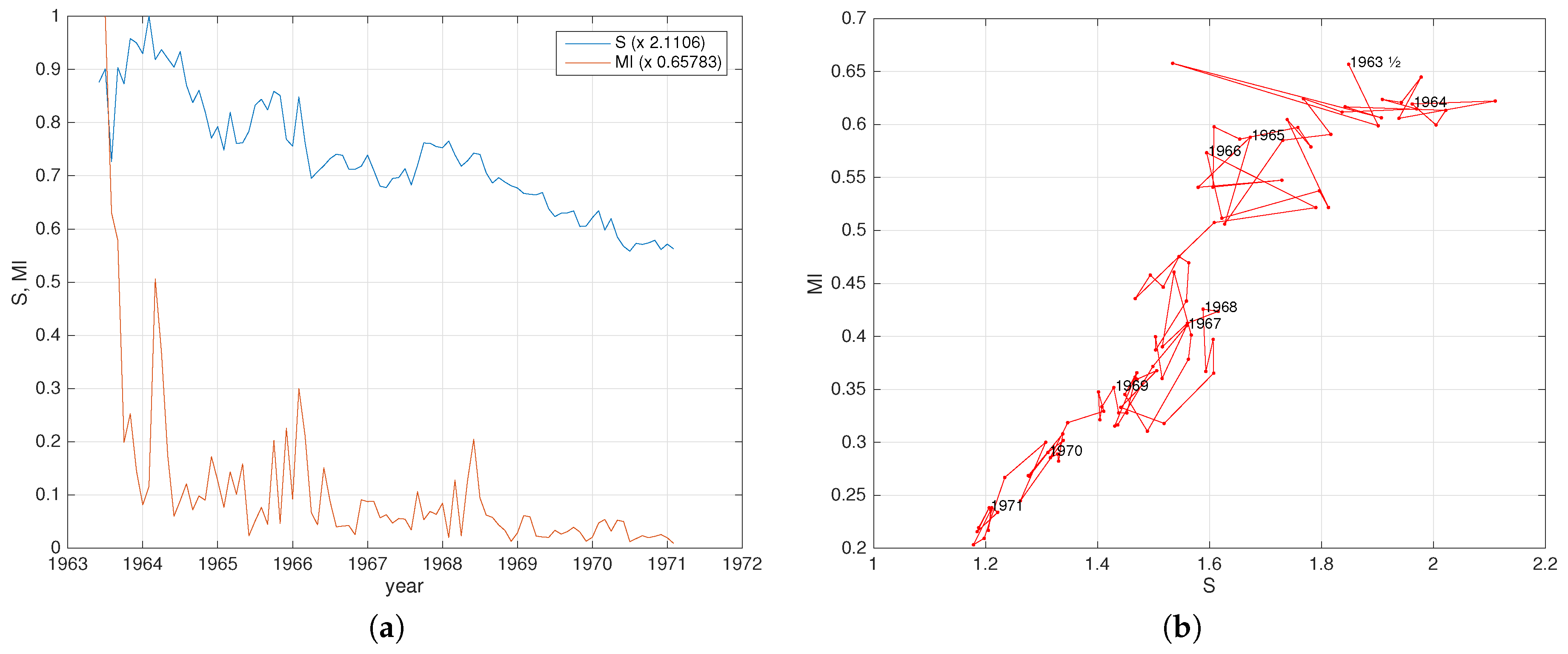
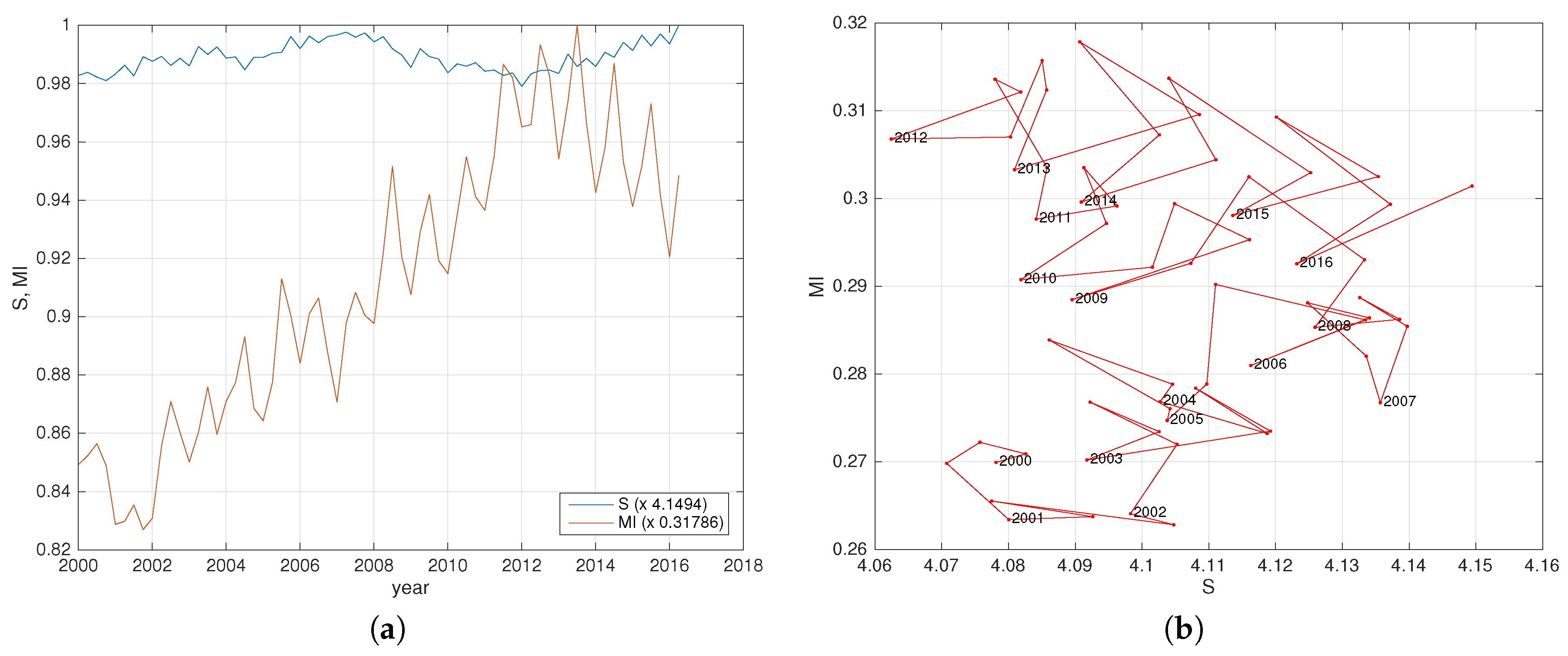
Figure 2 and Figure 8 show not only the entropy and mutual information variation in time, but also a state-space description .
For the EZMU (see Figure 2), we verify a decrease over time of both indices and that they exhibit a linear relationship in the locus . For the EMU (see Figure 8), we observe a limit cycle of with an approximate period of 10.4 years and an increase of I, up to a maximum in 2012, followed by a decrease until the present date. The state-space reveals a limit cycle with a one-year period and confirms that year 2012 was an extreme state, with the 2016 state close to that of 2008.
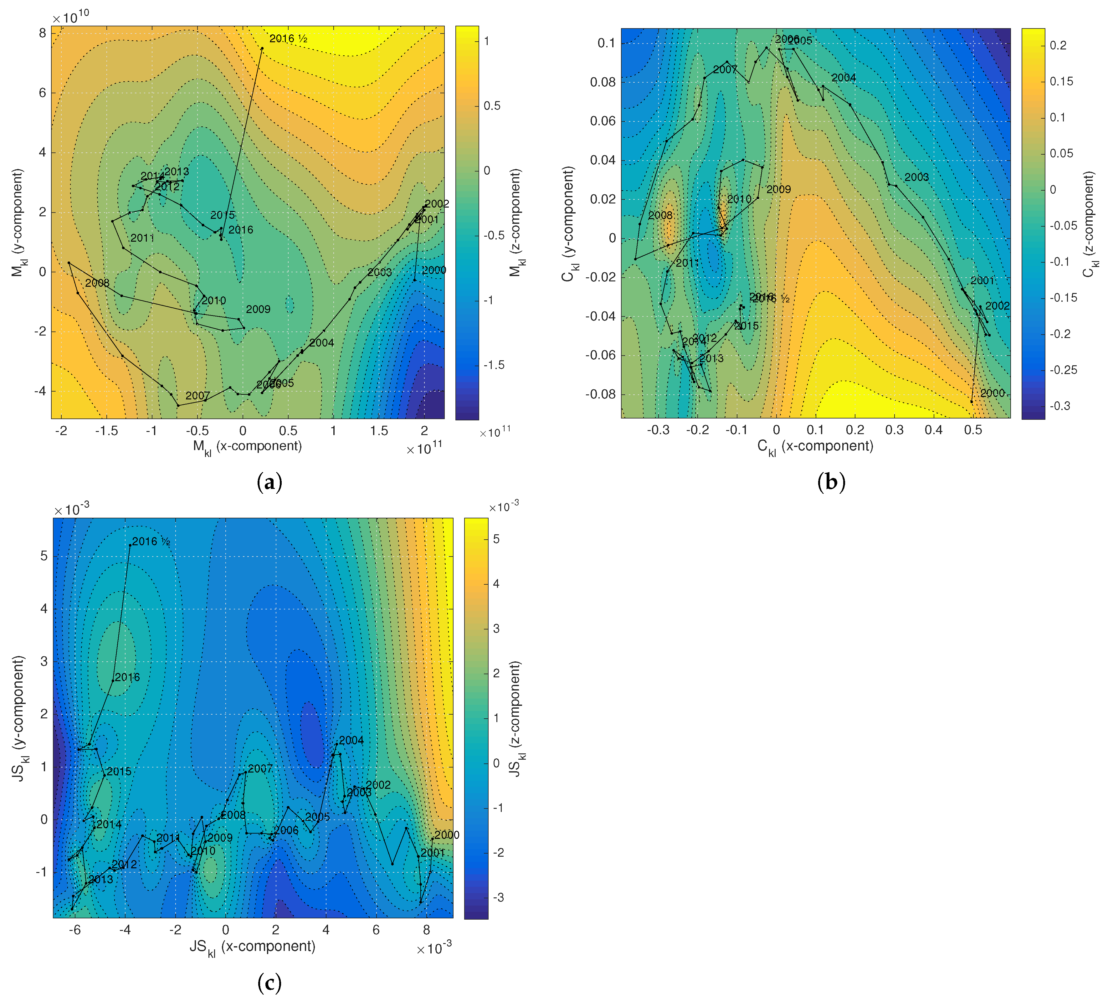
Figure 3 and Figure 9 depict the MDS charts produced by the indices during period . In both cases, we verify an evolution in which the successive states (i.e., the points) move away from the initial state. For smoothing the noise present in the trajectories, an average is adopted so that before calculating MDS, matrix G is filled by means of a moving average , and . It is interesting to note the influence of the four seasons, which is clear with the index for the EMU. Figure 4 and Figure 10 depict the corresponding two-dimensional MDS charts with the RBI technique.
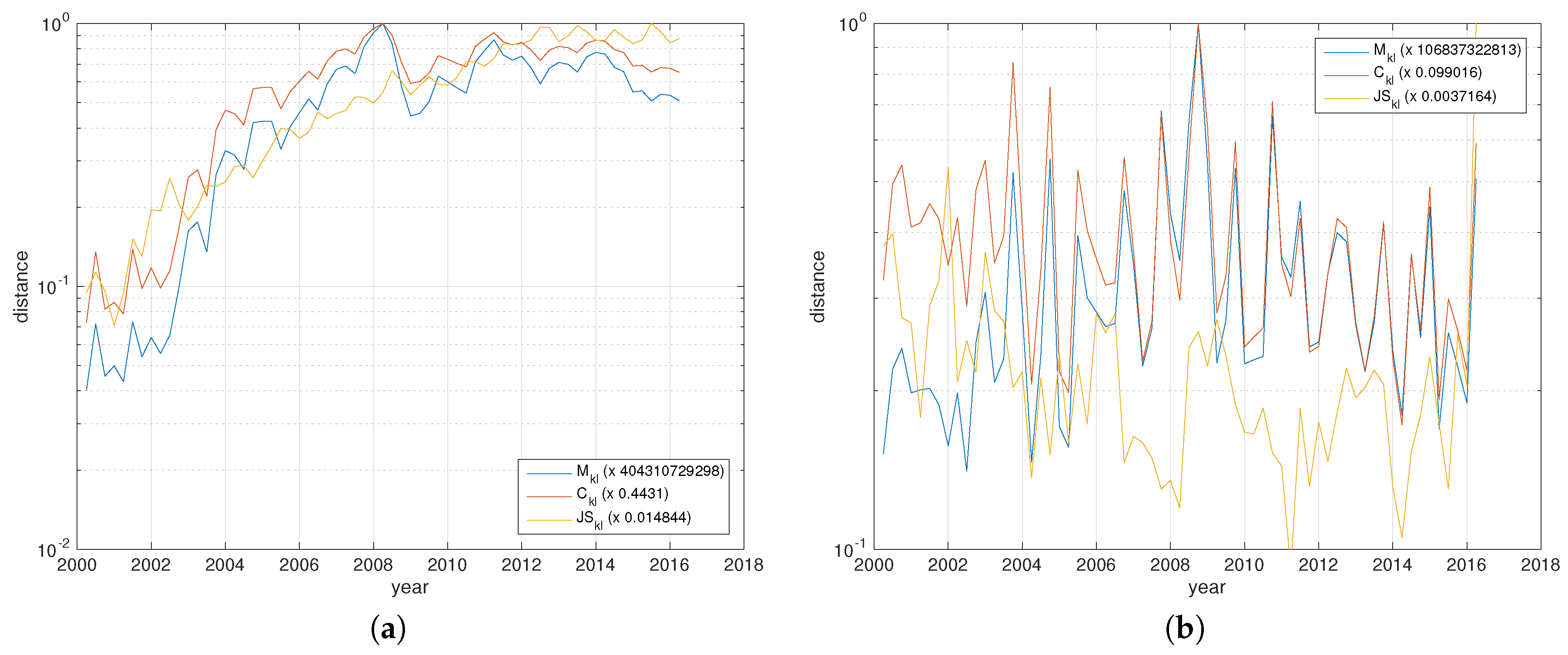
Figure 5 and Figure 11 represent the variation of the distances between the initial state at and the one at time t (left side), and the distances between the states at two consecutive instants, t and (right side). The two charts are consistent with the MDS plots, exhibiting an increasing distance from the initial state, but with a much more volatile variation in the case of the EMU.
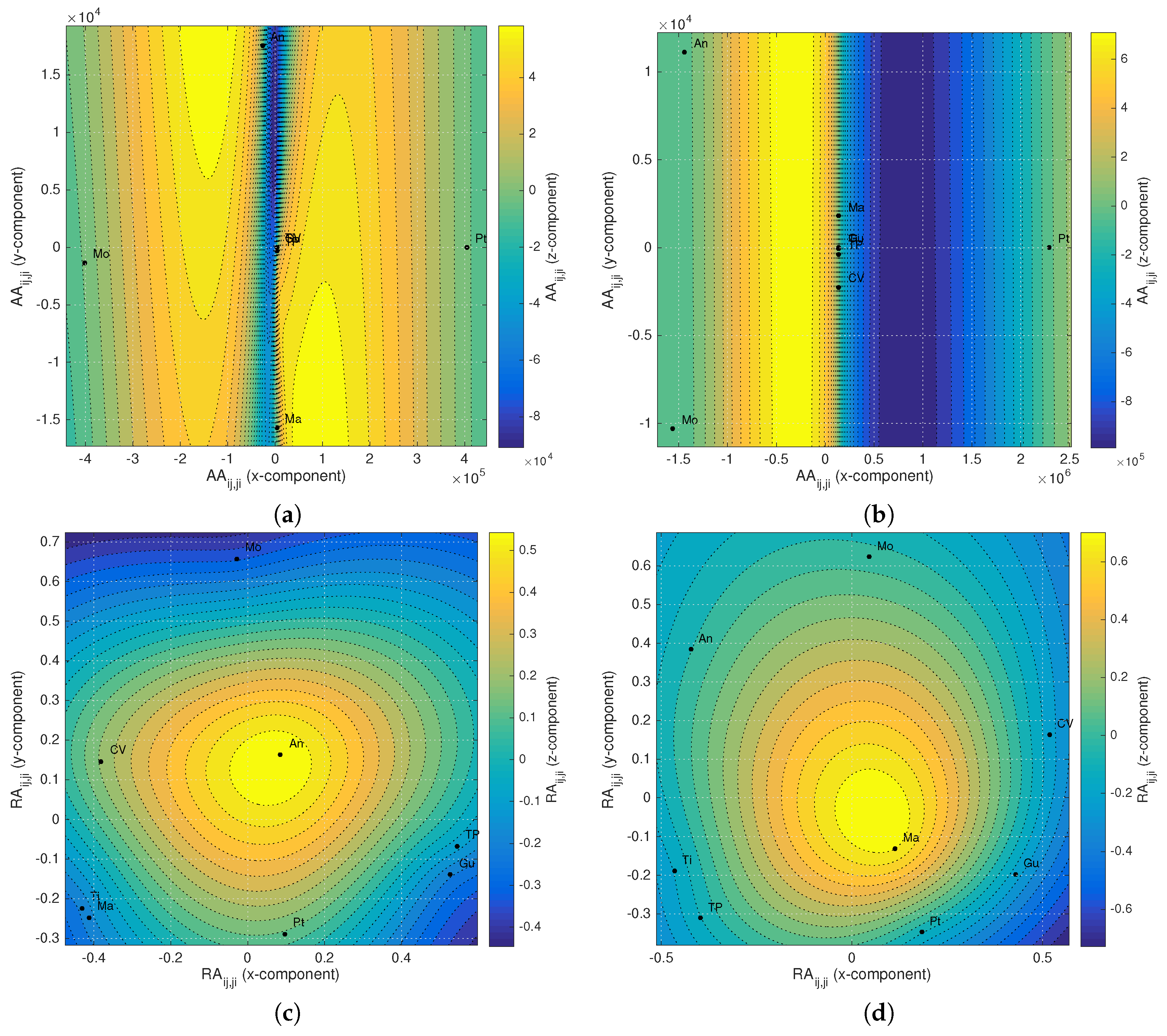
Figure 6 and Figure 7, Figure 12 and Figure 13 correspond to the MDS with RBI and “trees” produced by the HC and Phylip. For the sake of parsimony, we depict only the charts for time and . We observe that the quality of the map generated by is inferior to , particularly for the EZMU. Not only the MDS charts based on the depict a one-dimensional nature, but also the calculation of H yields a matrix with numerical values that are close to singular or badly scaled values so that results may be inaccurate. This result follows the initial estimate that the measures (4) and (8) would be sensitive to the presence of large and small values and that (5), (6) and (9) would be more robust.
It is possible to distinguish an initial period in both monetary unions. The Canberra distance for one quarter in the EMU and one month in the EZMU shows that compensation mechanisms were beginning to be checked. In both cases, political propaganda promised large benefits for participants, and expectations for the future were positive because of trade specialization and financial solidarity, thanks to commodities, labor, and free capital movements. The Canberra distance smoothed for one period and the Canberra distance for initial state makes clearer the special character of the initial period. In the case of the EZMU colonial terrorism activity and guerrilla warfare had two fronts (in Angola and Guinea), but the Government was hopeful for a victory by sending troops to these territories and investing in public utilities.
In 2002, the EMU euro currency was introduced and brought a stable character to intra-monetary union relationships, which lasted for about four years. In the case of the EZMU, it is also possible to see a smooth performance, while colonial terrorism affected the two territories only until 1964.
Divergence after the first period is quite clear in both EZMU and EMU. The unilateral declaration of independence of Rhodesia in November 1965, and sanctions against this country, coupled with terrorism attacks in Mozambique since 1966, led to a permanent Angolan and Mozambican indebtedness in the escudo compensation system creating the need for loans from the Portuguese motherland to respect the 1:1 parity. The period from then to 1968 thus changed the relative positions among the territories under Portuguese sovereignty. The same occurs with the EMU. In Europe, terrorism activity began to have some meaning [48], while successive partners joined in 2007 (Slovenia) and 2008 (Cyprus and Malta). Their presence in the euro community, coupled with other Southern partners’ net negative quarterly positions, brought asymmetrical profiles to the monetary EMU [49]. It became possible to identify more or less permanent debtor and creditor partners within the euro area. This reflected job market problems in many of these countries, as labor mobility faced several difficulties including language and cultural differences. These difficulties are usually identified with the 2008 crisis [50].
As for the EZMU, a post-1968 third stage is also quite clear, when a shift took place in the Portuguese society (Figure 5). Hopes for more liberal political relationships with the empire, thanks to the replacement of Prime-Minister Salazar by Marcelo Caetano led to lower levels of entropy in the system, as more and more motherland loans sought to accommodate rising levels of financial transfers to the colonies. Increasing Canberra distances for initial state and for end times characterize this phase that preceded the 1971 reform, which set back free trade and free capital flow. Angola, Mozambique, and Macao presented the most dissimilar positions, according to Canberra distance for end times (Figure 6 and Figure 7). Macao was the partner that most changed (in improving) from its initial position, and Angola the one that most changed (in losing) from its initial position (Figure 6). Decolonizations followed in 1974 for Guinea, and 1975 for the other African territories. Macao and Timor had opposite paths in the EZMU, from 1963 to 1971. Macao continued under Portuguese administration until 20 December 1999 and became a Chinese territory. Timor became independent on 20 May 2002, after a long and difficult international political process.
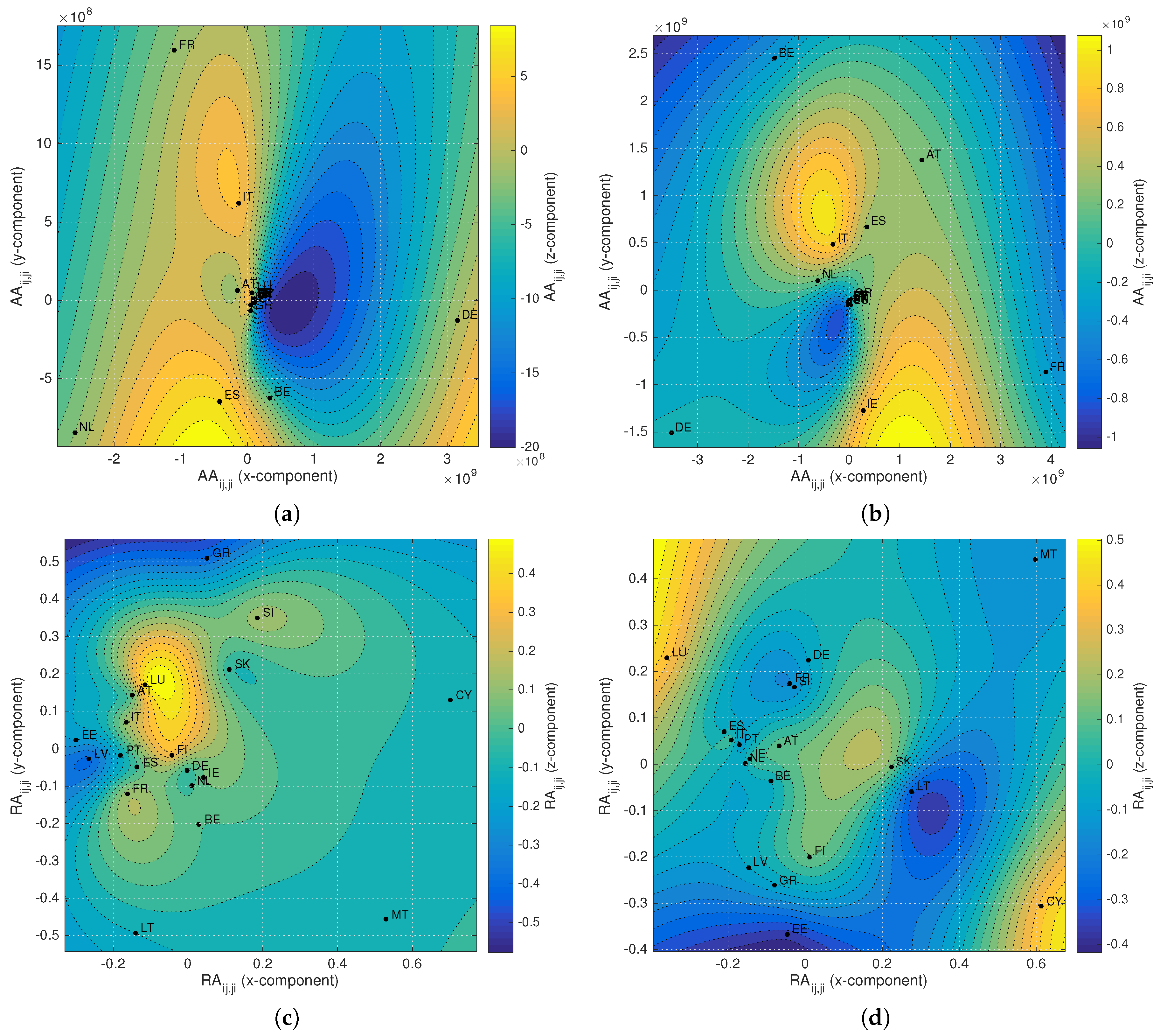
The MDS figures reveal that enlargements to new countries after 2008 also represent a third EMU phase. Coupled with terrorism activity and unrest in the EMU zone, and recent migration inflows because of warring in neighboring countries, they have contributed to added dissimilarity in net relative positions. Slovakia joined on 1 January 2009, the Baltic Estonia on 1 January 2011, Latvia in 2014, and Lithuania in 2015 [51]. The Canberra distance for initial state and for end time reveal a disruption with increasing levels of entropy (Figure 9). The relative good performance of Luxembourg and the poor performance of Cyprus are totally opposite (see Figure 12 and Figure 13).
In 2016, the EMU core similarity includes Austria, Belgium, Luxembourg, France, Germany, Ireland, Italy, Netherlands, Portugal, Spain, and Slovenia. A second group of countries presents high dissimilarity, namely, Malta, the Slovak Republic, Finland, Greece, Latvia, and Lithuania, as well as Cyprus and Estonia, according to Figure 13.
4. Conclusions
This paper presented a modeling approach of economic unions based on real-world data. We started with a small case, the EZMU, and followed with a larger case, the EMU. For analyzing the data, we adopted techniques employed in complex systems, namely, entropy, Canberra distance, and Jensen–Shannon divergence, combined with computational and visualization techniques, MDS and HC. The results for the EZMU and EMU are different, but consistent with existing heuristic knowledge. The use of several distinct measures is essential to capture the different features of the complex dynamics involved in the monetary unions.
According to the evidence from MDS techniques and pictures, it becomes easier to describe how and why a reform of the EZMU was introduced in 1971, and how and why the need of a reform for the EMU is often mentioned. Databases clearly point to evolutions that exhibit strongly divergent net positions among the partners in both monetary unions. In spite of economic and monetary integration, Mundell’s expected automatic mechanisms for self-regulation and equilibrium are not historically confirmed. They may be disrupted by political problems such as terrorism, migrations from the outside instead of internal migrations, and negative expectations on the success of compensating monetary systems. The EZMU failed and the EMU is far from an OCA. MDS empirically checks the evidence on two case studies, one made of independent partners (the EMU), and another made of politically-related territories, and disappoints theories that stress the importance of political ties for monetary unions’ success. OCAs depend not only on the mobility of factors, but also on the symmetry of disturbances caused by them, so that permanent debtors (and creditors) can not arise in the process [52]. This is a central debate for scholars and policy-makers.
Acknowledgments
We are grateful to the Bank of Portugal Historical Archives, for Maria Eugénia Mata’s access to data on the Escudo Zone Monetary Union, and to John Huffstot for improving our English.
Author Contributions
Maria Eugénia Mata and Jose Tenreiro Machado conceived, designed, and performed the experiments. Maria Eugénia Mata and Jose Tenreiro Machado analyzed the data and wrote the paper. Maria Eugénia Mata contributed with the data. All authors have read and approved the final version of the manuscript.
Conflicts of Interest
The authors declare no conflict of interest.
References
- Peters, E.E. Fractal Market Analysis: Applying Chaos Theory to Investment and Economics; John Wiley & Sons: New York, NY, USA, 1994. [Google Scholar]
- Nahorski, Z.; Ravn, H.F. A review of mathematical models in economic environmental problems. Ann. Oper. Res. 2000, 97, 165–201. [Google Scholar] [CrossRef]
- Filar, J.A.; Krawczyk, J.B. (Eds.) Mathematical Models in Economics, Vol. 3; UNESCO: Paris, France, 2009. [Google Scholar]
- Hritonenko, N.; Yatsenko, Y. Mathematical Modeling in Economics, Ecology and the Environment; Springer: New York, NY, USA, 2013. [Google Scholar]
- Mutanov, G. Mathematical Methods and Models in Economic Planning, Management and Budgeting; Springer: New York, NY, USA, 2015. [Google Scholar]
- Johansen, S. Confronting the Economic Model with the Data; Cambridge University Press: Cambridge, UK, 2006; pp. 287–300. [Google Scholar]
- Machado, J.A.T.; Mata, M.E. Pseudo Phase Plane and Fractional Calculus Modelling of Western Global Economic Downturn. Commun. Nonlinear Sci. Numer. Simul. 2015, 22, 396–406. [Google Scholar] [CrossRef]
- Machado, J.A.T.; Mata, M.E. Analysis of World Economic Variables Using Multidimensional Scaling. PLoS ONE 2015, 10, e0121277. [Google Scholar] [CrossRef] [PubMed]
- Machado, J.A.T.; Mata, M.E. A Fractional Perspective to the Bond Graph Modelling of World Economies. Nonlinear Dyn. 2015, 80, 1839–1852. [Google Scholar] [CrossRef]
- Machado, J.A.T.; Mata, M.E.; Lopes, A.M. Fractional State Space Analysis of Economic Systems. Nonlinear Dyn. 2015, 17, 5402–5421. [Google Scholar] [CrossRef]
- Dibeh, G. A Kaleckian model of business cycle synchronization. Rev. Political Econ. 2005, 17, 253–267. [Google Scholar] [CrossRef]
- Eickmeier, S.; Breitung, J. How Synchronized Are Central and East European Economies with the Euro Area? Evidence from a Structural Factor Model; Discussion Paper 20/2005; Deutsche Bundesbank: Frankfurt, Germany, 2005. [Google Scholar]
- Chian, A.C.L.; Borotto, F.A.; Rempel, E.L.; Rogers, C. Attractor merging crisis in chaotic business cycles. Chaos Solitons Fractals 2005, 24, 869–875. [Google Scholar] [CrossRef]
- Naldi, G.; Pareschi, L.; Toscani, G. (Eds.) Mathematical Modeling of Collective Behavior in Socio-Economic and Life Sciences; Springer Science & Business Media: Berlin, Germany, 2010. [Google Scholar]
- Bouali, S.; Buscarino, A.; Fortuna, L.; Frasca, M.; Gambuzza, L. Emulating complex business cycles by using an electronic analogue. Nonlinear Anal. Real World Appl. 2012, 13, 2459–2465. [Google Scholar] [CrossRef]
- Kalemli-Ozcan, S.; Papaioannou, E.; Peydró, J.L. Financial Regulation, Financial Globalization, and the Synchronization of Economic Activity. J. Financ. 2013, 68, 1179–1228. [Google Scholar] [CrossRef]
- Xi, N.; Muneepeerakul, R.; Azaele, S.; Wang, Y. Maximum entropy model for business cycle synchronization. Physica A 2014, 413, 189–194. [Google Scholar] [CrossRef]
- Abraham, R.; Nivala, M. Chaotic Synchronization and the Global Economy. IIM Kozhikode Soc. Manag. Rev. 2014, 2, 157–163. [Google Scholar] [CrossRef]
- Juvenal, L.; Monteiro, P.S. Trade and synchronization in a multi-country economy. Eur. Econ. Rev. 2017, 92, 385–415. [Google Scholar] [CrossRef]
- Swoboda, A. Robert Mundell and the Theoretical Foundation for the European Monetary Union; Technical Report; International Monetary Fund: Washington, DC, USA, 1999. [Google Scholar]
- Johnson, H.G.; Swoboda, A.K. The Economics of Common Currencies: Proceedings of the Madrid Conference on Optimum Currency Areas; Allen & Unwin: London, UK, 1973. [Google Scholar]
- Grauwe, P.D. Monetary union and convergence economics. Eur. Econ. Rev. 1996, 40, 1091–1101. [Google Scholar] [CrossRef]
- Mundell, R.A. A theory of optimum currency areas. Am. Econ. Rev. 1961, 51, 657–665. [Google Scholar]
- Shannon, C.E. A Mathematical Theory of Communication. Bell Syst. Tech. J. 1948, 27, 379–423, 623–656. [Google Scholar] [CrossRef]
- Shannon, C.E. Information Theory and Statistical Mechanics. Phys. Rev. 1957, 106, 620–630. [Google Scholar]
- Khinchin, A.I. Mathematical Foundations of Information Theory; Dover Publications: Mineola, NY, USA, 1957. [Google Scholar]
- Rényi, A. On measures of information and entropy. In Proceedings of the Fourth Berkeley Symposium on Mathematics, Statistics and Probability, Berkeley, CA, USA, 20–30 June 1960; pp. 547–561. [Google Scholar]
- Rathie, P.N.; Silva, S.D. Shannon, Levy, and Tsallis: A Note. Appl. Math. Sci. 2008, 2, 1359–1363. [Google Scholar]
- Gray, R.M. Entropy and Information Theory; Springer: New York, NY, USA, 2009. [Google Scholar]
- Machado, J.A.T. Fractional Order Generalized Information. Entropy 2014, 16, 2350–2361. [Google Scholar] [CrossRef]
- Jeffreys, H. An Invariant Form for the Prior Probability in Estimation Problems. Proc. R. Soc. Lond. Ser. A Math. Phys. Sci. 1946, 186, 453–461. [Google Scholar] [CrossRef]
- Kullback, S.; Leibler, R.A. On Information and Sufficiency. Ann. Math. Stat. 1951, 22, 79–86. [Google Scholar] [CrossRef]
- Lin, J. Divergence measures based on the Shannon entropy. IEEE Trans. Inf. Theory 1991, 37, 145–151. [Google Scholar] [CrossRef]
- Gordon, A. Classification, Second Edition (Monographs on Statistics and Applied Probability, 82); Chapman & Hall/CRC: London, UK, 1999. [Google Scholar]
- Taneja, I.J. Generalized Information Measures and Their Applications; Universidade Federal de Santa Catarina: Florianópolis, Brazil, 2001. [Google Scholar]
- Cha, S.H. Comprehensive Survey on Distance/Similarity Measures between Probability Density Functions. Int. J. Math. Models Methods Appl. Sci. 2007, 1, 300–307. [Google Scholar]
- Deza, M.M.; Deza, E. Encyclopedia of Distances; Springer: Berlin/Heidelberg, Germany, 2009. [Google Scholar]
- Torgerson, W.S. Theory and Methods of Scaling; John Wiley and Sons: New York, NY, USA, 1958. [Google Scholar]
- Kruskal, J. Multidimensional scaling by optimizing goodness of fit to a nonmetric hypothesis. Psychometrika 1964, 29, 1–27. [Google Scholar] [CrossRef]
- Shepard, R.N. The analysis of proximities: Multidimensional scaling with an unknown distance function. I. Psychometrika 1962, 27, 125–140. [Google Scholar] [CrossRef]
- Shepard, R.N. The analysis of proximities: Multidimensional scaling with an unknown distance function. II. Psychometrika 1962, 27, 219–246. [Google Scholar] [CrossRef]
- Sammon, J. A nonlinear mapping for data structure analysis. IEEE Trans. Comput. 1969, 18, 401–409. [Google Scholar] [CrossRef]
- Kruskal, J.B.; Wish, M. Multidimensional Scaling, 11th ed.; Sage: Newbury Park, CA, USA, 1978. [Google Scholar]
- Cox, T.F.; Cox, M.A.A. Multidimensional Scaling; Chapman & Hall/CRC: Boca Raton, FL, USA, 2001. [Google Scholar]
- Borg, I.; Groenen, P.J. Modern Multidimensional Scaling: Theory and Applications; Springer: New York, NY, USA, 2005. [Google Scholar]
- Carr, J.C.; Fright, W.R.; Beatson, R.K. Surface interpolation with radial basis functions for medical imaging. IEEE Trans. Med. Imaging 1997, 16, 96–107. [Google Scholar] [CrossRef] [PubMed]
- PHYLIP: The PHYLogeny Inference Package. Available online: http://evolution.genetics.washington.edu/phylip.html (accessed on 18 May 2017).
- Lopes, A.M.; Machado, J.T.; Mata, M.E. Analysis of global terrorism dynamics by means of entropy and state space portrait. Nonlinear Dyn. 2016, 85, 1547–1560. [Google Scholar] [CrossRef]
- Funke, M. The Nature of Shocks in Europe and in Germany. Economica 1997, 64, 461–469. [Google Scholar] [CrossRef]
- Decressina, J.; Fatás, A. Regional labour market dynamics in Europe. Eur. Econ. Rev. 1995, 39, 1627–1655. [Google Scholar] [CrossRef]
- Bayoumi, T.; Eichengreen, B. Is There a Conflict between EC enlargement and European Monetary Unification? Working Paper 3950; National Bureau of Economic Research: Cambridge, MA, USA, 1992. [Google Scholar]
- Blanchard, O.J.; Quah, D. The Dynamic Effects of Aggregate Demand and Supply Disturbances. Am. Econ. Rev. 1989, 79, 655–673. [Google Scholar]
Figure 1.
Computational visualization scheme.
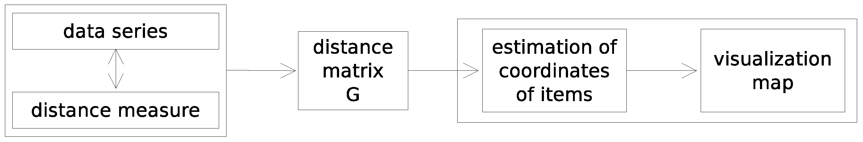
Figure 2.
Analysis of the EZMU during the years 1963–1971 using the joint entropy S and mutual information I: (a) Time evolution of and ; (b) state space representation .
Figure 2.
Analysis of the EZMU during the years 1963–1971 using the joint entropy S and mutual information I: (a) Time evolution of and ; (b) state space representation .

Figure 3.
MDS charts with of the EZMU during the years 1963–1971 using the: (a) Manhattan distance, ; (b) Canberra distance, ; (c) Jensen–Shannon divergence, .
Figure 3.
MDS charts with of the EZMU during the years 1963–1971 using the: (a) Manhattan distance, ; (b) Canberra distance, ; (c) Jensen–Shannon divergence, .
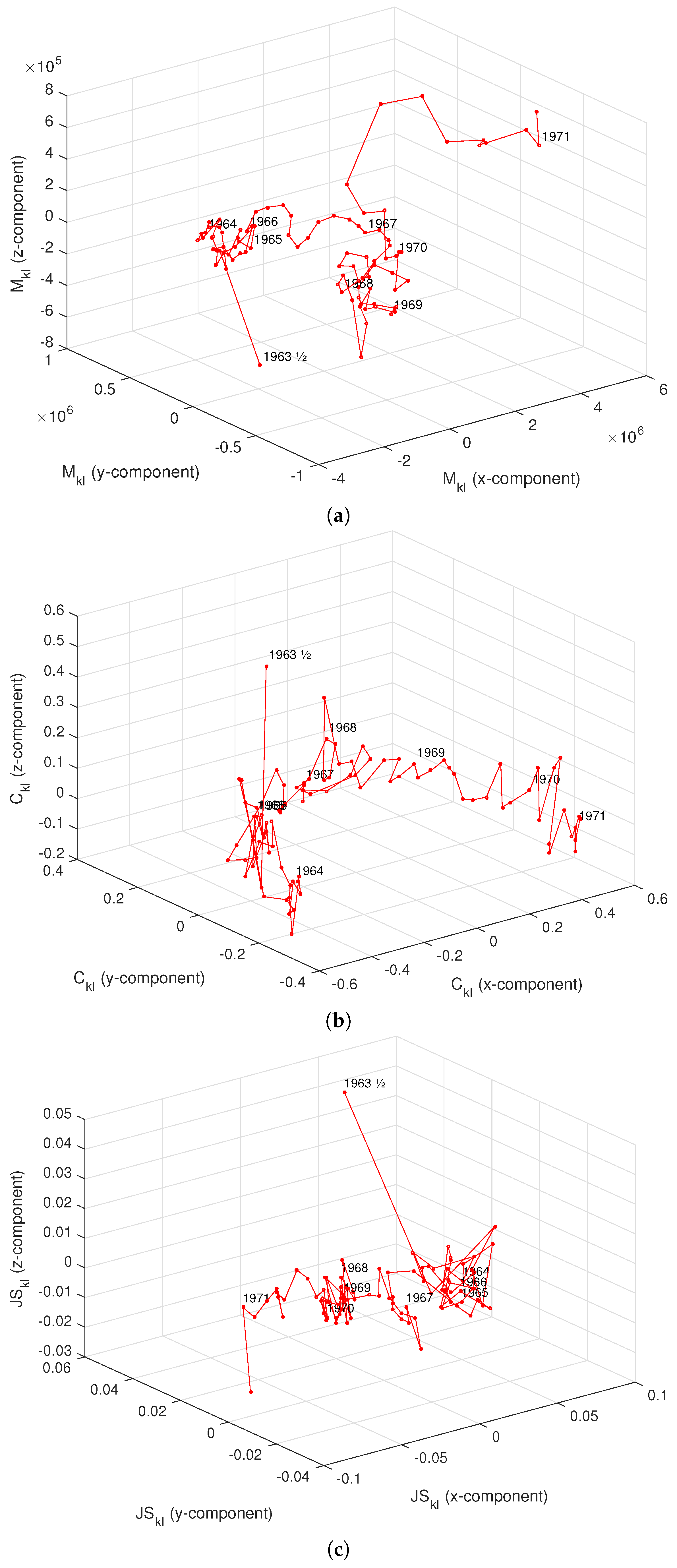
Figure 4.
MDS charts with and RBI of the EZMU during the years 1963–1971 using the: (a) the Manhattan distance, ; (b) Canberra distance, ; (c) Jensen–Shannon divergence, .
Figure 4.
MDS charts with and RBI of the EZMU during the years 1963–1971 using the: (a) the Manhattan distance, ; (b) Canberra distance, ; (c) Jensen–Shannon divergence, .
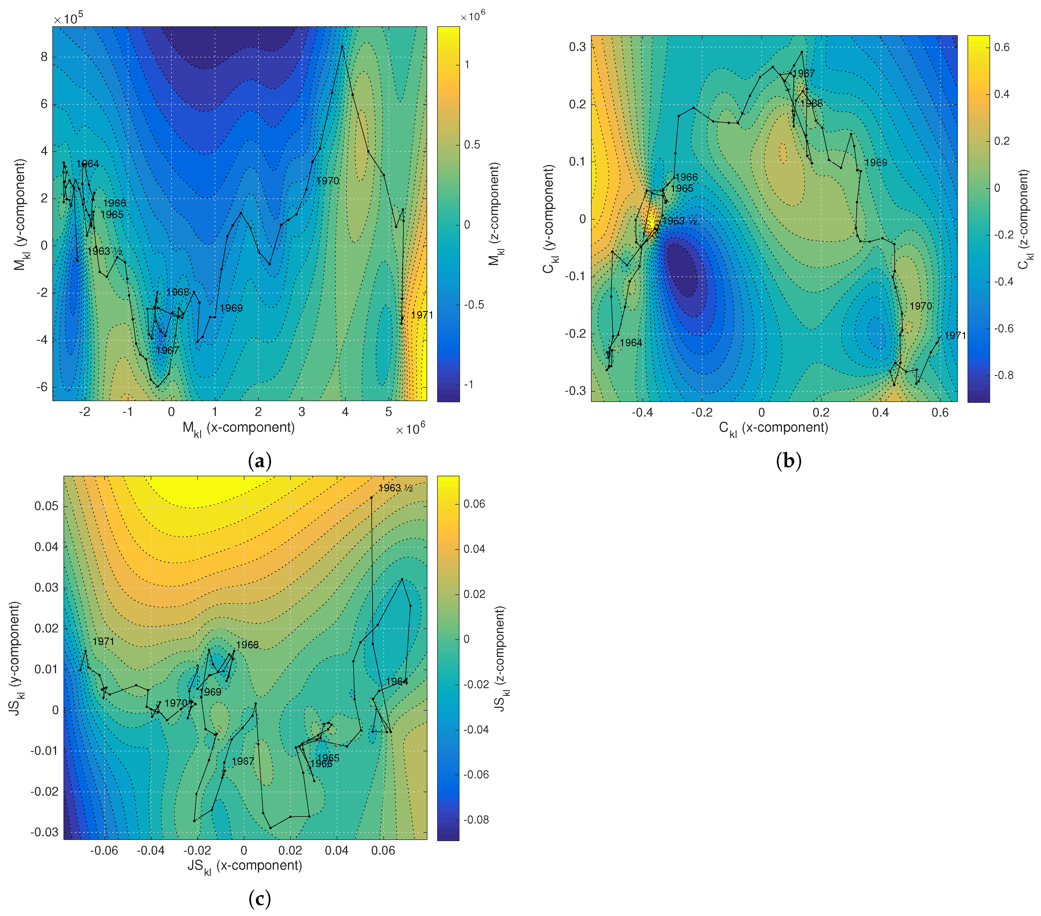
Figure 5.
Analysis of the EZMU evolution during the years 1963–1971 using the Manhattan distance (), Canberra distance () and Jensen–Shannon divergence (). Comparison between: (a) two states at time and ; (b) two consecutive states at time t and .
Figure 5.
Analysis of the EZMU evolution during the years 1963–1971 using the Manhattan distance (), Canberra distance () and Jensen–Shannon divergence (). Comparison between: (a) two states at time and ; (b) two consecutive states at time t and .
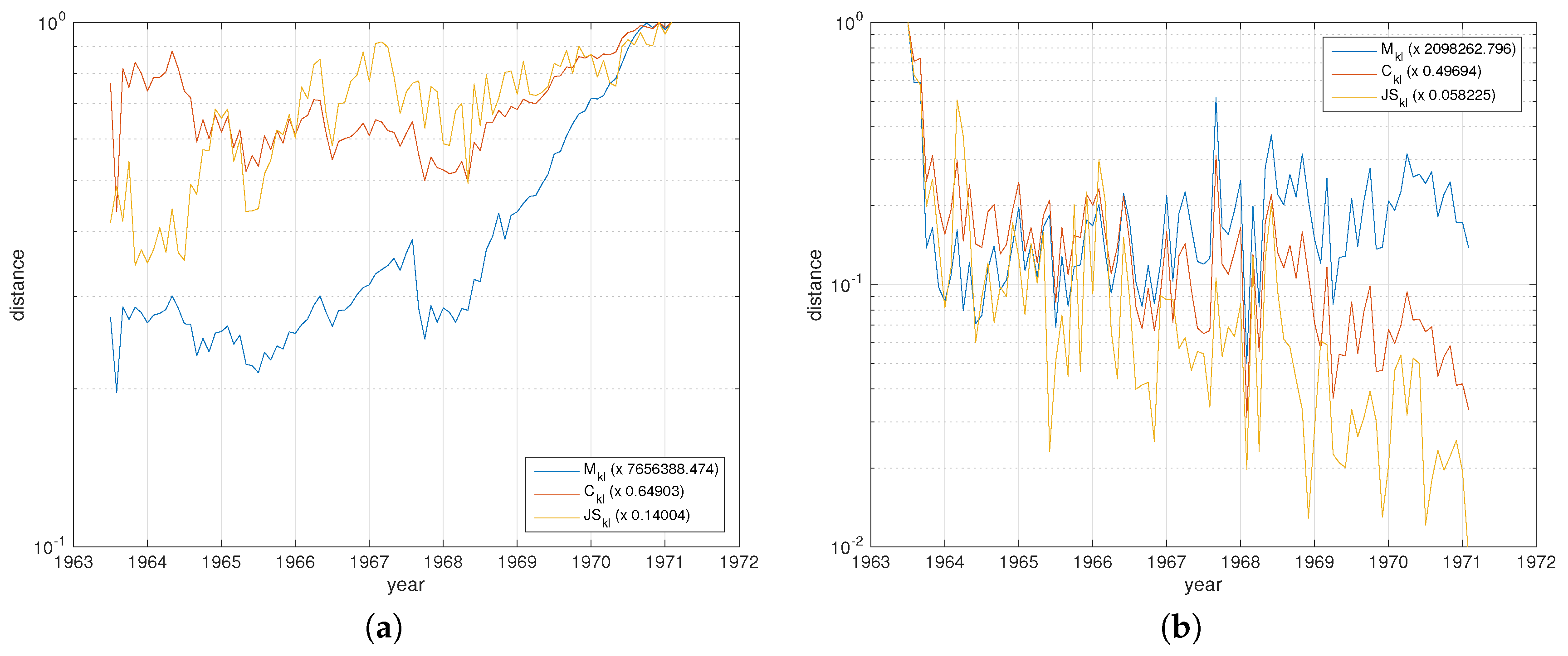
Figure 6.
MDS charts with and RBI of the relationship between the EZMU countries in and using asymmetry measures. (a) , ; (b) , ; (c) , ; (d) , .
Figure 6.
MDS charts with and RBI of the relationship between the EZMU countries in and using asymmetry measures. (a) , ; (b) , ; (c) , ; (d) , .

Figure 7.
HC charts of the relationship between the EZMU countries in and using asymmetry measures. (a) , ; (b) , ; (c) , ; (d) , .
Figure 7.
HC charts of the relationship between the EZMU countries in and using asymmetry measures. (a) , ; (b) , ; (c) , ; (d) , .
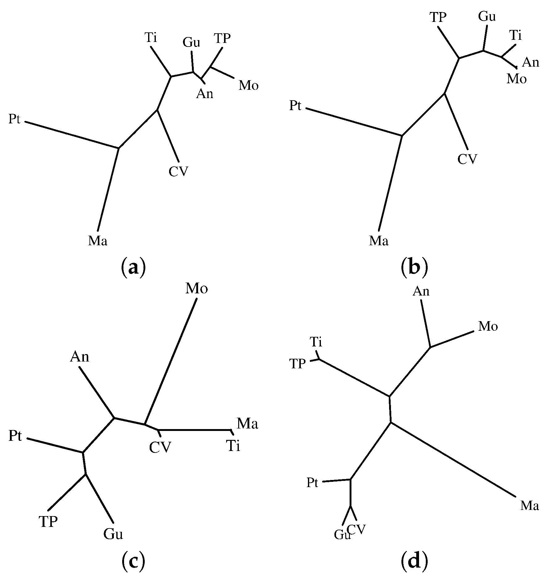
Figure 8.
Analysis of the EMU during the years 2000–2016 using the joint entropy S and mutual information I. (a) Time evolution of and ; (b) state space representation .
Figure 8.
Analysis of the EMU during the years 2000–2016 using the joint entropy S and mutual information I. (a) Time evolution of and ; (b) state space representation .

Figure 9.
MDS charts with of the EMU during the years 2000–2016 using the: (a) Manhattan distance, ; (b) Canberra distance, ; (c) Jensen–Shannon divergence, .
Figure 9.
MDS charts with of the EMU during the years 2000–2016 using the: (a) Manhattan distance, ; (b) Canberra distance, ; (c) Jensen–Shannon divergence, .
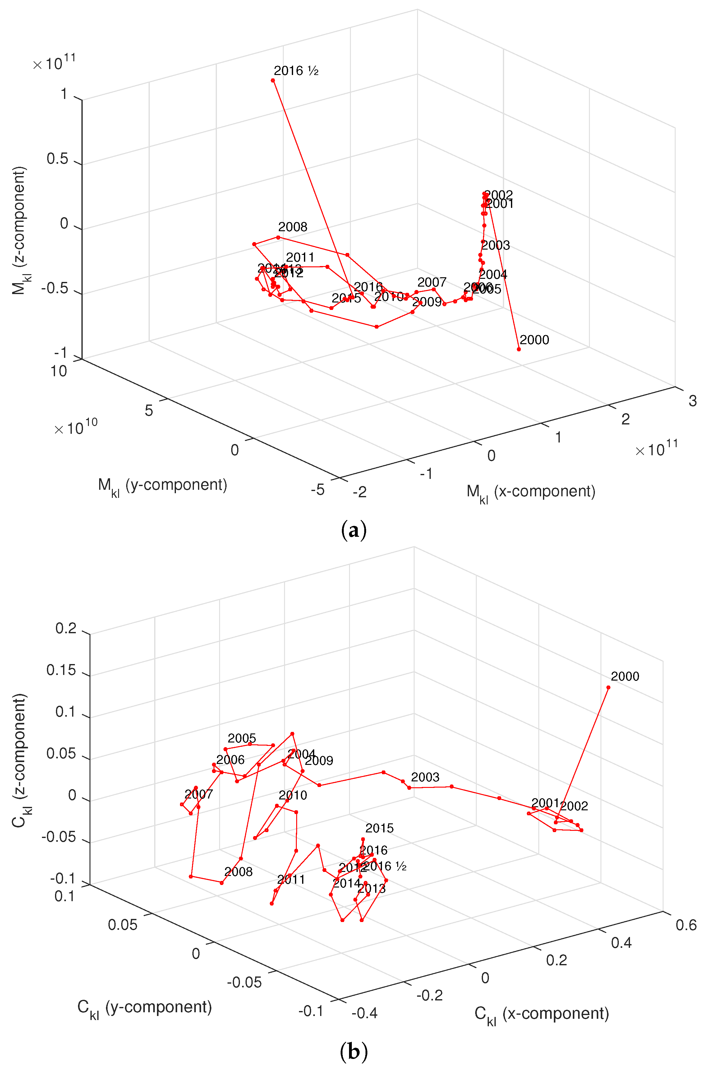
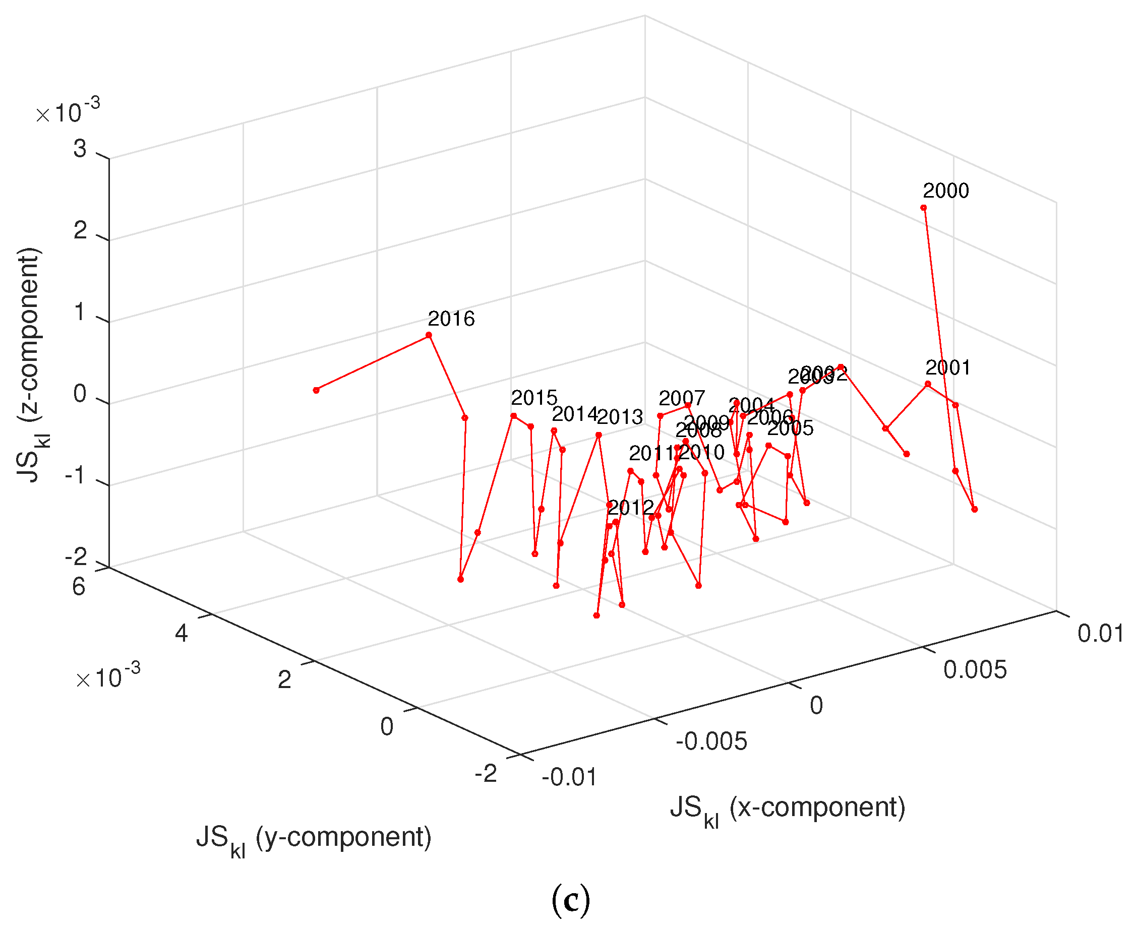
Figure 10.
MDS charts with and RBI of the EMU during the years 2000–2016 using the: (a) Manhattan distance, ; (b) Canberra distance, ; (c) Jensen–Shannon divergence, .
Figure 10.
MDS charts with and RBI of the EMU during the years 2000–2016 using the: (a) Manhattan distance, ; (b) Canberra distance, ; (c) Jensen–Shannon divergence, .

Figure 11.
Analysis of the EMU evolution during the years 2000–2016 using the Manhattan distance (), Canberra distance () and Jensen–Shannon divergence (). Comparison between: (a) two states at time and ; (b) two consecutive states at time t and .
Figure 11.
Analysis of the EMU evolution during the years 2000–2016 using the Manhattan distance (), Canberra distance () and Jensen–Shannon divergence (). Comparison between: (a) two states at time and ; (b) two consecutive states at time t and .

Figure 12.
MDS charts with and RBI of the relationship between the EMU countries in and using asymmetry measures. (a) , ; (b) , ; (c) , ; (d) , .
Figure 12.
MDS charts with and RBI of the relationship between the EMU countries in and using asymmetry measures. (a) , ; (b) , ; (c) , ; (d) , .

Figure 13.
HC charts of the relationship between the EMU countries in and using asymmetry measures. (a) , ; (b) , ; (c) , ; (d) , .
Figure 13.
HC charts of the relationship between the EMU countries in and using asymmetry measures. (a) , ; (b) , ; (c) , ; (d) , .


Table 1.
The EZMU Timeline.
| Date | Description |
|---|---|
| 1961 | First terrorism actions in Angola |
| November 1961 | Decree-law 44016: Foundation of the escudo monetary zone |
| 1962 | Decree-laws 44698, 44701, 44702: Framing the background for all the monetary features
The beginning data of the EZMU operation: BoP assumed much wider functions in order to be the central bank of the whole system of compensation payments among all territories under |
| March 1963 | Portuguese political sovereignty and administration. A new contract was signed with the Portuguese central state (through the Ministry of Finance). New contracts between the other issuing banks and contracts with the Portuguese central state (through the Ministry of Finance) were also signed |
| 1963 | Beginning of terrorism and guerrilla warfare in Guinea |
| 1964 | Beginning of terrorism and guerrilla warfare in Mozambique, intensifying after 1966 |
| September 1968 | Prime minister Salazar’s illness and replacement by Marcelo Caetano
Reform the EZMU: it introduced quantitative restrictions, tariffs, and previous authorization |
| November 1971 | on commodities imported from abroad. Exports were submitted to a previous registration in bulletins. The colonial Exchange Funds also were authorized to issue domestic loans with state guarantee, but they were jointly responsible for them |
| 1974–1975 | Decolonization |
Table 2.
The EMU Timeline.
| Date | Description |
|---|---|
| July 1990 | Exchange controls were abolished, and capital movements were completely liberalized |
| 1992 | The Treaty of Maastricht established the economic convergence criteria concerning the inflation rate, public finances, interest rates, and exchange rate stability |
| December 1995 | The name of the new currency (the euro) and the duration of the transition periods were decided |
| June 1997 | Definition of a Stability and Growth Pact to ensure budgetary discipline after creation of the euro |
| June 1998 | Foundation of European Central Bank (ECB) |
| December 1998 | Definition of the conversion rates between the 11 participating national currencies and the euro |
| 1999 | The euro became a real currency, and the ECB assumed a single monetary policy |
| January 2002 | The euro notes and coins were introduced |
| 2004–2005 | Madrid and London terrorism attacks |
| January 2007 | Slovenia joins the EMU |
| January 2008 | Cyprus and Malta join the EMU |
| January 2009 | Slovakia joins the EMU |
| January 2011 | Estonia joins the EMU |
| January 2014 | Latvia joins the EMU |
| January 2015 | Lithuania joins the EMU |
| 2015–2016 | Paris, Brussels, Nice, Berlin terrorism attacks and Migrant crisis in Europe |
© 2017 by the authors. Licensee MDPI, Basel, Switzerland. This article is an open access article distributed under the terms and conditions of the Creative Commons Attribution (CC BY) license (http://creativecommons.org/licenses/by/4.0/).
Share and Cite
MDPI and ACS Style
Mata, M.E.; Machado, J.T. Entropy Analysis of Monetary Unions. Entropy 2017, 19, 245. https://doi.org/10.3390/e19060245
AMA Style
Mata ME, Machado JT. Entropy Analysis of Monetary Unions. Entropy. 2017; 19(6):245. https://doi.org/10.3390/e19060245
Chicago/Turabian StyleMata, Maria Eugénia, and Jose Tenreiro Machado. 2017. "Entropy Analysis of Monetary Unions" Entropy 19, no. 6: 245. https://doi.org/10.3390/e19060245
Note that from the first issue of 2016, this journal uses article numbers instead of page numbers. See further details here.