5.2. Experimental Setup
Our framework is implemented in Python using the Theano library [
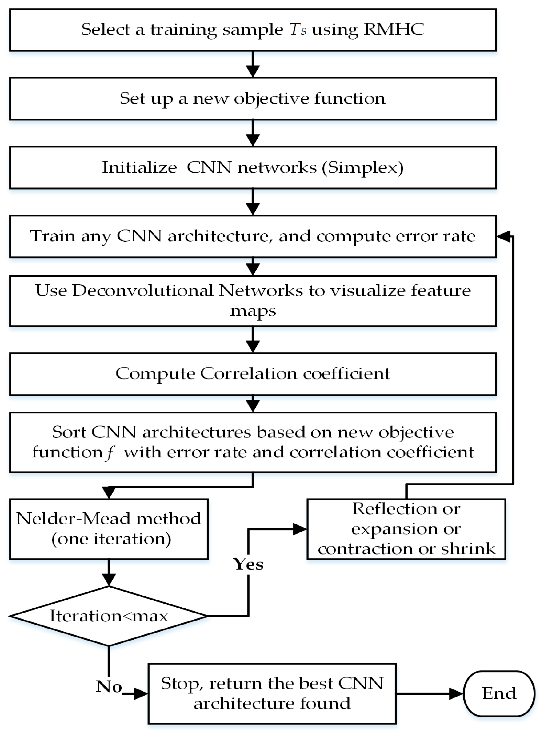
73] to train the CNN models. Theano provides automatic differentiation capabilities to compute gradients and allows the use of GPU to accelerate the computation. During the exploration phase via NMM, we select a training sample
TS using an RMHC algorithm with a sample size based on a margin error of 1 and confidence level of 95%. Then, we select 8000 images randomly from (
TTR–
TS) for validation set
TV.
Training Settings: We use SGD to train CNN architectures. The final learning rate is set to 0.08 for 25 epochs and 0.008 for the last epochs; these values are selected after doing a small grid search among different values on the validation set. We set the batch size to 32 images and the weight decay to 0.0005. The weights of all layers are initialized according to the Xavier initialization technique [
42], and biases are set to zero. The advantage of Xavier initialization is that it makes the network converge much faster than other approaches. The weight sets it produces are also more consistent than those produced by other techniques. We apply ReLU with all layers and employ early stopping to prevent overfitting in the performance of the validation set. Once the error rate increases or saturates for a number of iterations, the model stops the training procedure. Since the training time of a CNN is expensive and some designs perform poorly, early stopping saves time by terminating poor architecture designs early. Dropout [
11] is implemented with fully-connected layers with a rate of 0.5. It has proven to be an effective method in combating overfitting in CNNs, and a rate of 0.5 is a common practice. During the exploration phase of NMM, each of the experiments are run with 35 epochs. Once the best CNN architecture is obtained, we train it with the training set
TTR and evaluate it on a testing set with 200 epochs.
Nelder Mead Settings: The total number of hyperparameters
n is required to construct the initial simplex with
n + 1 vertices. However, this number is different for each dataset. In order to define
n for a given dataset, we initialize 80 random CNN architectures as an additional step to return the maximum number of convolutional layers (
Cmax) in all architectures. Then, according to Equation (4), the number of hyperparameters
n is given by:
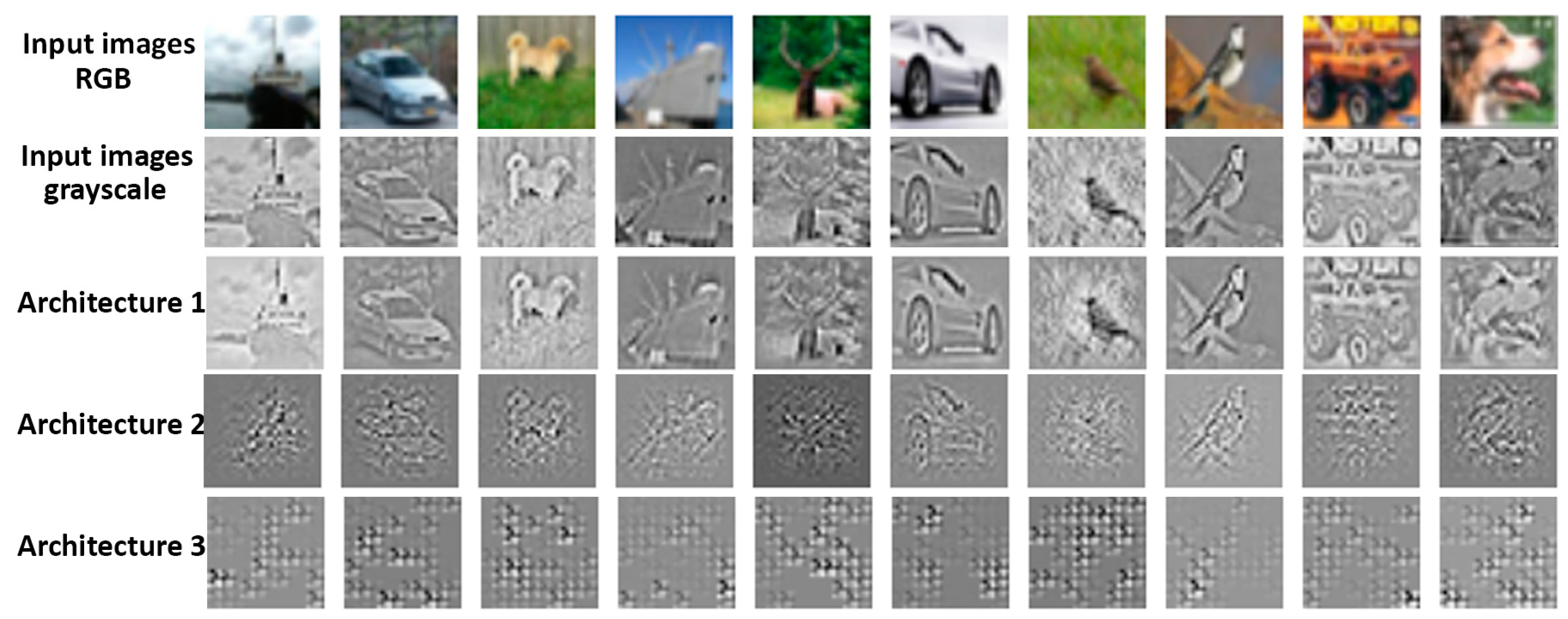
NMM will then initialize a new initial simplex (Z0) with n + 1 vertices. For all datasets, we set the value of the correlation coefficient parameter to = 0.20. We select at random Nfm = 10 feature maps from the last convolutional layer to visualize their learned features and Nimg = 100 images from the training sample to assess the visualization. The number of iterations for NMM is 25.
Table 1 summarizes the hyperparameter initialization ranges for the initial simplex vertices (CNN architectures) of NMM. The number of convolutional layers is calculated automatically by subtracting the depth from the number of fully-connected layers. However, the actual number of convolutional layers is controlled by the size of the input image, filter sizes, strides and pooling region sizes according to Equations (1) and (2). Some CNN architectures may not result in feasible configurations based on initial hyperparameter selections, because after a set of convolutional layers, the size of feature maps (
W) or pooling (
P) may become <1, so the higher convolutional layers will be automatically eliminated. Therefore, the depth varies through CNN architectures; this will be helpful to optimize the depth. There is no restriction on fully-connected layers. For example, the hyperparameters of the following CNN architecture are initialized randomly from
Table 1, which consists of six convolutional layers and two fully-connected layers as follows:
For an input image of size 32 × 32, the framework designs a CNN architecture with only three convolutional layers because the output size of a fourth layer would be negative. Thus, the remaining convolutional layers from the fourth layer will be deleted automatically by setting them to zeros as shown below:
5.3. Results and Discussion
First, we validate the effectiveness of the proposed objective function compared to the error rate objective function. After initializing a simplex (Z
0) of NMM, we optimize the architecture using NMM based on the proposed objective function (error rate as well as visualization). Then, from the same initialization (Z
0), we execute the NMM based on the error rate objective function alone by setting
to zero.
Table 2 compares the error rate of five experiment runs obtained from the best CNN architectures found using the objective functions presented above on the CIFAR-10 and CIFAR-100 datasets respectively. The results illustrate that our new objective function outperforms the optimization obtained from the error rate objective function alone. The error rate averages of 15.87% and 40.70% are obtained with our objective function, as compared to 17.69% and 42.72% when using the error rate objection function alone, on CIFAR-10 and CIAFAR-100 respectively. Our objective function searches the architecture that minimizes the error and improves the visualization of learned features, which impacts the search space direction, and thus produces a better CNN architecture.
We also compare the performance of our approach with existing methods that did not apply data augmentation, namely hand-designed architectures by experts, random search, genetic algorithms, and Bayesian optimization. For CIFAR-10, [
72] reported that the best hand-crafted CNN architecture design tuned by human experts obtained an 18% error rate. In [
22], genetic algorithms are used to optimize filter sizes and the number of filters for convolutional layers; it achieved a 25% error rate. In [
74], SMAC is implemented to optimize the number of filters, filter sizes, pooling region sizes, and fully-connected layers with a fixed depth. They achieved an error rate of 17.47%. As shown in
Table 3, our method outperforms others with an error rate of 15.27%. For CIFAR-100, we implement random search by picking CNN architectures from
Table 1, and the lowest error rate that we obtained is 44.97%. In [
74], which implemented SMAC, an error rate of 42.21% is reported. Our approach outperforms these methods with an error rate of 40.12%, as shown in
Table 3.
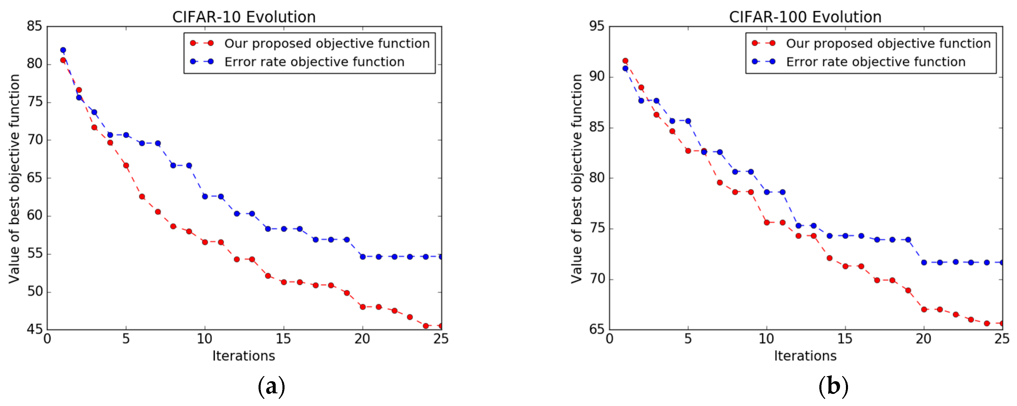
In each iteration of NMM, a better-performing CNN architecture is potentially discovered that minimizes the value of the objective function; however, it can get stuck in a local minimum.
Figure 6 shows the value of the best CNN architecture versus the iteration using both objective functions, i.e., the objective function based on error rate alone and our new, combined objective function. In many iterations, NMM paired with the error rate objective function is unable to pick a new, better-performing CNN architecture and gets stuck in local minima early. The number of architectures that yield a higher performance during the optimization process is only 12 and 10 out of 25, on CIFAR-10 and CIFAR-100 respectively. In contrast, NMM with our new objective function is able to explore better-performing CNN architectures with a total number of 19 and 17 architectures on CIFAR-10 and CIFAR-100 respectively, and it does not get stuck early in a local minimum, as shown in
Figure 6b. The main hallmark of our new objective function is that it is based on both the error rate and the correlation coefficient (obtained from the visualization of the CNN via deconvnet), which gives us flexibility to sample a new architecture, thereby improving the performance.
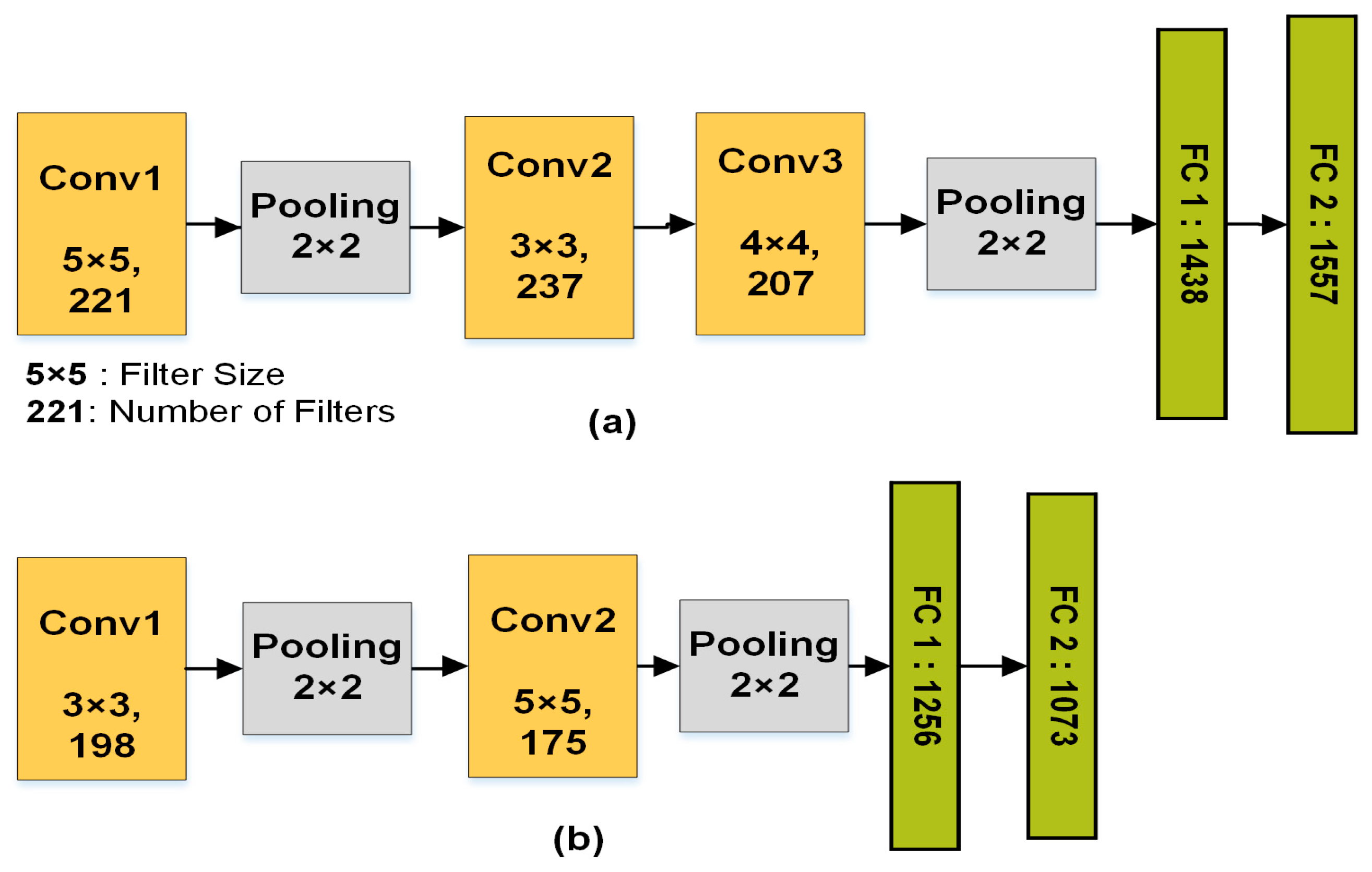
We further investigated the characteristics of the best CNN architectures obtained by both objective functions using NMM on CIFAR-10 and CIFAR-100. We took the average of the hyperparameters of the best CNN architectures. As shown in
Figure 7a, CNN architectures based on the proposed framework tend to be deeper compared to architectures obtained by the error rate objective function alone. Moreover, some convolutional layers are not followed by pooling layers. As a result, we found that reducing the number of pooling layers shows a better visualization, and results in adding more layers. On the other hand, the architectures obtained by the error objective function alone result in every convolutional layer being followed by a pooling layer.
We compare the run-time of NMM on a single computer with a parallel NMM algorithm on three distributed computers. The running time decreases almost linearly (3×) as the number of workers increases, as shown in
Table 4. In a synchronous master-slave NMM model, the master cannot move to the next step until all of the workers finish their jobs, so other workers wait until the biggest CNN architecture training is done. This creates a minor delay. In addition, the run-time of
Corr based on Equation (6) is 0.05 s; when based on FFT in Equation (7), it is 0.01 s.
We compare the performance of our approach with state-of-the-art results and recent works on architecture search on three datasets. As seen in
Table 5, we achieve competitive performance on the MNIST dataset in comparison to the state-of-the-art results, with an error rate 0.42%. The results on CIFAR-10 and CIFAR-100 are obtained after applying data augmentation. Recent architecture search techniques [
49,
50,
51,
52] show good results; however, these promising results were only possible with substantial computation resources and a long execution time. For example, GA [
51] used genetic algorithms to discover the network architecture for a given task. Each experiment was distributed to over 250 parallel workers. Ref. [
49] used reinforcement learning (RL) to tune a total of 12,800 different architectures to find the best on CIFAR-10, and the task took over three weeks. However, our framework uses only three workers and requires tuning an average of 260 different CNN architectures in around one day. It is possible to run our framework on a single computer. Therefore, our approach is comparable to the state-of-the-art results on CIFAR-10 and CIFAR-100, because our results require significantly fewer resources and less processing time. Some methods such as Residential Networks (ResNet) [
15] achieve state-of-the-art results because the structure is different than a CNN. However, it is possible to implement our framework in ResNet to find the best architecture.
To test the robustness of the selection of the training sample, we compared a random selection against RMHC for the same sample size; we found that RMHC achieved better results by about 2%. We found that our new objective function is very effective in guiding a large search space into a sub-region that yields a final, high-performing CNN architecture design. Pooling layers and large strides show a poor visualization, so our framework restricts the placement of pooling layers: It does not follow every convolutional layer with a pooling layer, which shrinks the size of the strides. Moreover, this results in increased depth. We found that the framework allows navigation through a large search space without any restriction on depth until it finds a promising CNN architecture. Our framework can be implemented in other problem domains where images and visualization are involved, such as image registration, detection, and segmentation.


