
An Entropy-Based Generalized Gamma Distribution for Flood Frequency Analysis

1
College of Hydropower and Information Engineering, Huazhong University of Science and Technology, Wuhan 430074, China
2
Department of Biological and Agricultural Engineering, Texas A&M University, College Station, TX 77843, USA
3
Zachry Department of Civil Engineering, Texas A&M University, College Station, TX 77843, USA
4
State Key Laboratory of Water Resources and Hydropower Engineering Science, Wuhan University, Wuhan 430072, China
*
Author to whom correspondence should be addressed.
Entropy 2017, 19(6), 239; https://doi.org/10.3390/e19060239
Submission received: 17 April 2017
/
Revised: 17 May 2017
/
Accepted: 19 May 2017
/
Published: 2 June 2017
(This article belongs to the Special Issue Entropy Applications in Environmental and Water Engineering)
Abstract
:Flood frequency analysis (FFA) is needed for the design of water engineering and hydraulic structures. The choice of an appropriate frequency distribution is one of the most important issues in FFA. A key problem in FFA is that no single distribution has been accepted as a global standard. The common practice is to try some candidate distributions and select the one best fitting the data, based on a goodness of fit criterion. However, this practice entails much calculation. Sometimes generalized distributions, which can specialize into several simpler distributions, are fitted, for they may provide a better fit to data. Therefore, the generalized gamma (GG) distribution was employed for FFA in this study. The principle of maximum entropy (POME) was used to estimate GG parameters. Monte Carlo simulation was carried out to evaluate the performance of the GG distribution and to compare with widely used distributions. Finally, the T-year design flood was calculated using the GG and compared with that with other distributions. Results show that the GG distribution is either superior or comparable to other distributions.
1. Introduction
Flood frequency analysis (FFA) is needed for the design of water engineering and hydraulic structures. The sizing of bridges, culverts and other facilities; the design capacities of levees, spillways and other control structures; and reservoir operation or management all depend upon the estimated magnitude of various design flood values [1,2,3]. In FFA, flow data, such as the annual maximum data, are fitted using a theoretical frequency distribution, which is usually selected from a set of candidate distributions [4]. For example, the Pearson type three distribution (P3) has been recommended in China [5]. In the US, since 1967 the Log-Pearson type 3 distribution (LP3) has been the official distribution for all catchments which are fitted for planning and insurance purposes [6]. The UK has endorsed the GEV distribution [7,8] for FFA.
The choice of the appropriate model is one of the most important issues for FFA. The method commonly practiced is to try different distributions for the data at hand and choose the best fitted distribution using some particular goodness-of-fit measure [9]. One of the disadvantages of this method is that too many different distributions need to be tried and the selected distribution may be the best based on one goodness of fit criterion, but not based on another criterion. In order to overcome this disadvantage, some generalized frequency distributions have been recently used for FFA. The generalized gamma (GG) distribution is discussed in this study. It is a generalization of the two-parameter gamma distribution. The GG distribution includes as special cases the exponential distribution, the two-parameter gamma distribution, and the Weibull distribution, which provide sufficient flexibility to fit a large variety of data sets.
After deciding the distribution, the second issues is to estimate the parameters associated with the GG distribution. The popular techniques for parameter estimation include the methods of maximum likelihood (ML) [7], moments (MM) [10] and L-moments [11]. In addition, entropy theory can be used to derive more generalized distributions using different constraints [12]. The theory involves entropy maximizing in accord with the principle of maximum entropy (POME), in which the distribution parameter are determined, given the observed data and a set of constraints. Singh [12] indicated that the entropy method was reasonable and efficient for parameter estimation.
The objective of this study was therefore to propose an entropy based generalized gamma distribution for flood frequency analysis. The GG distribution parameters were estimated using POME. The GG distribution was tested using observed data sets. Also, Monte Carlo simulation was carried out to evaluate the predictive ability of the GG distribution and it was compared with some widely accepted distributions. Finally, the T-year design flood values were calculated and compared based on different FFA distributions.
2. Methodology
2.1. Generalized Gamma Distribution
Let X be a random variable and x be its specific value. The probability density function (PDF) of the generalized gamma (GG) distribution can be expressed as:
where Γ(•) is the gamma function, and r1, r2 are the shape parameters, and β is the scale parameter.
2.2. Estimation of Parameters of GB2 Distribution by POME
The GG distribution parameters were determined using the principle of maximum entropy (POME). The POME method involves the following steps: (1) specification of constraints; (2) maximization of entropy using the method of Lagrange multipliers; (3) derivation of the relation between Lagrange multipliers and constraints; (4) derivation of the relation between Lagrange multipliers and distribution parameters; and (5) derivation of the relation between distribution parameters and constraints. A flow chart showing the estimation procedure is shown in Figure 1.
2.2.1. Specification of Constraints
Flood discharge is considered as a random variable X, which ranges from 0 to infinity. Its probability distribution function (PDF) and cumulative distribution function (CDF) are denoted as f(x) and F(x), respectively, where x is a specific value of X. Since constraints encode the information that can be given for the random variable, following Singh [12], the constraints for the GG distribution can be expressed as:
The first constraint is the total probability law, the second constraint is the mean of log values or the geometric mean, and the third constraint is the mean of values raised to a power q or log of scaled values raised to a power and then shifted by unity.
2.2.2. Maximization of Entropy Using the Method of Lagrange Multipliers
The f(x) can be obtained by maximizing the Shannon entropy subject to given constraints in accord with the principle of maximum entropy (POME). Following Singh [14,15], maximization of Equation (3), subject to Equation (2a) to (2c), using the method of Lagrange multipliers leads to:
where λ0, λ1, λ2 are the Lagrange multipliers that are not known.
2.2.3. Relation between Lagrange multipliers and parameters
Substitution of Equation (4) in Equation (2a) yields:
Equation (5) can be expressed as:
Let . Then , and . Then Equation (6) can be expressed as:
Substitution of Equation (7) in Equation (4) yields:
Let , and . Then, r2 = q, and r1 = −λ1 + 1. Equation (8) can now be written as:
Equation (9) is the same as the generalized gamma distribution given by Equation (1). Hence, the relation between Lagrange multipliers and distribution parameters are given by:
2.2.4. Relation between Lagrange Multipliers and Constraints
Since the Lagrange multiplier λ0 can be expressed by Equations (6) and (7), the set of equations can be used to obtain λ0:
Differentiation of Equation (11a) with respect to λ1 and λ2 yields:
Defining , and differentiating Equation (11b) with respect to λ1 and λ2, we obtain:
where φ(•)is a digamma function.
Based on Equations (12) and (13), the relation between Lagrange multipliers and constraints can be expressed as:
Since there are three parameters, Equations (13) and (14) are not sufficient for calculating all the parameters, and one additional equation is therefore needed which is given as:
2.2.5. Relation between Parameters and Constraints
Based on the relation between parameters and constraints and between parameters and Lagrange multipliers, the relation between parameters and constraints can be expressed as:
where φ(•) is the digamma function; φ'(•) is the tri-gamma function. For a given data set X, the E(lnx) and var(lnx) can be calculated directly. There are three parameters and three equations in Equation (16). Therefore, this set of nonlinear functions can be solved by the widely used Newton iteration method (Deuflhard, [16]) for parameter estimation. The initial value of the three parameters are set to (1, 1, 1). After multiple iterations, the optimal parameters can be obtained.
3. The Descriptive Ability of GG Distribution
Annual maximum (AM) flood peak data from 10 gauging stations, namely sites 1 to 10, were selected (Table 1). These ten stations are selected due to their diversity of statistical properties and climate types (arid, semi-arid and humid).
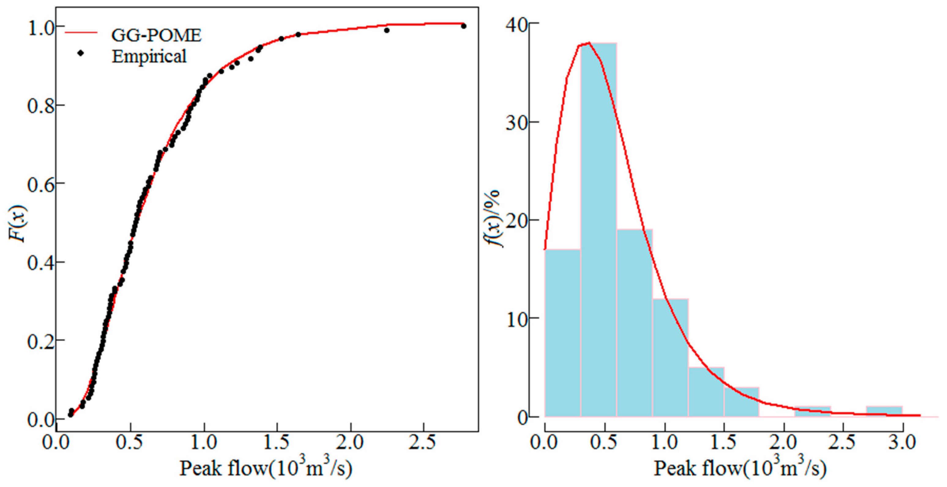
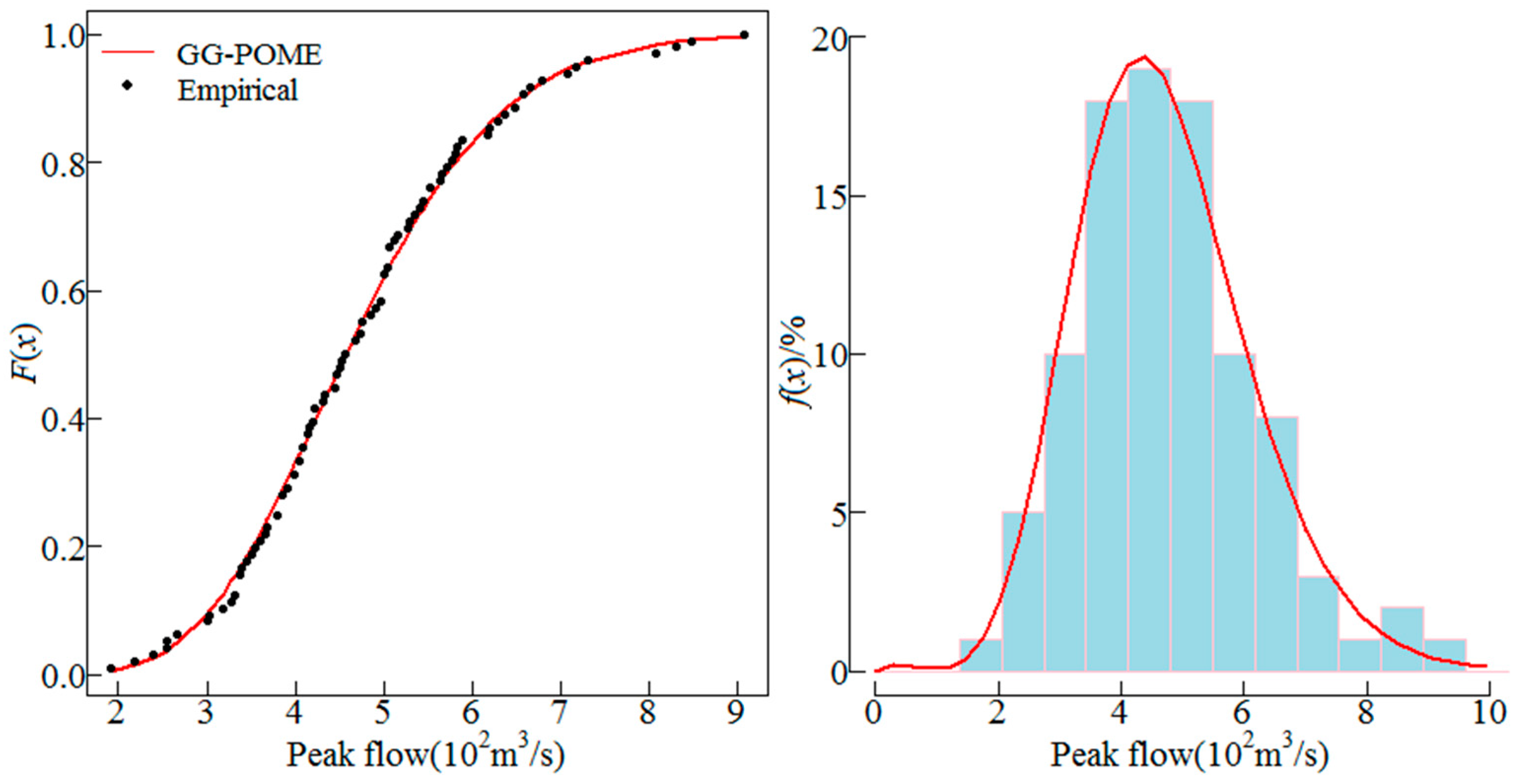
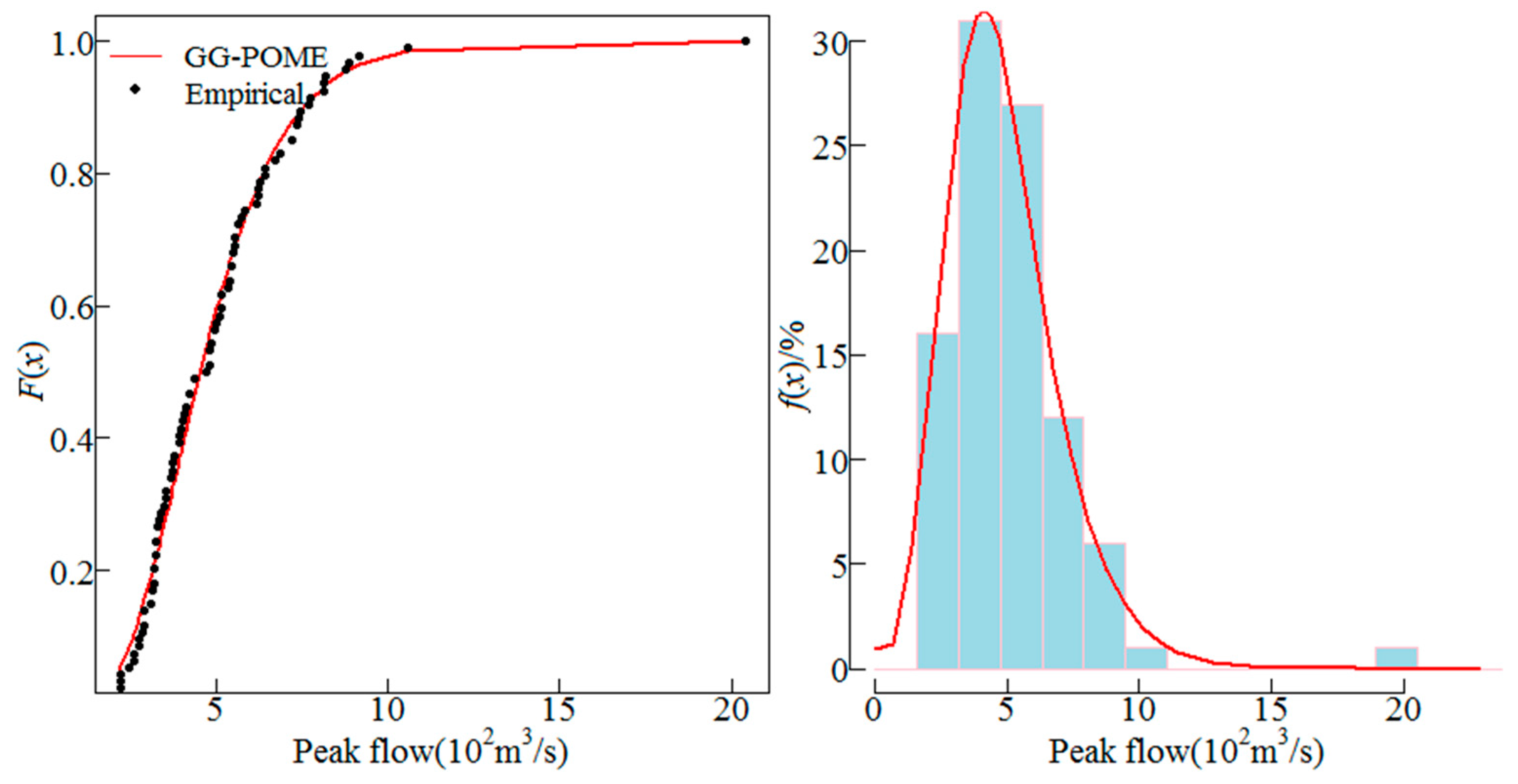
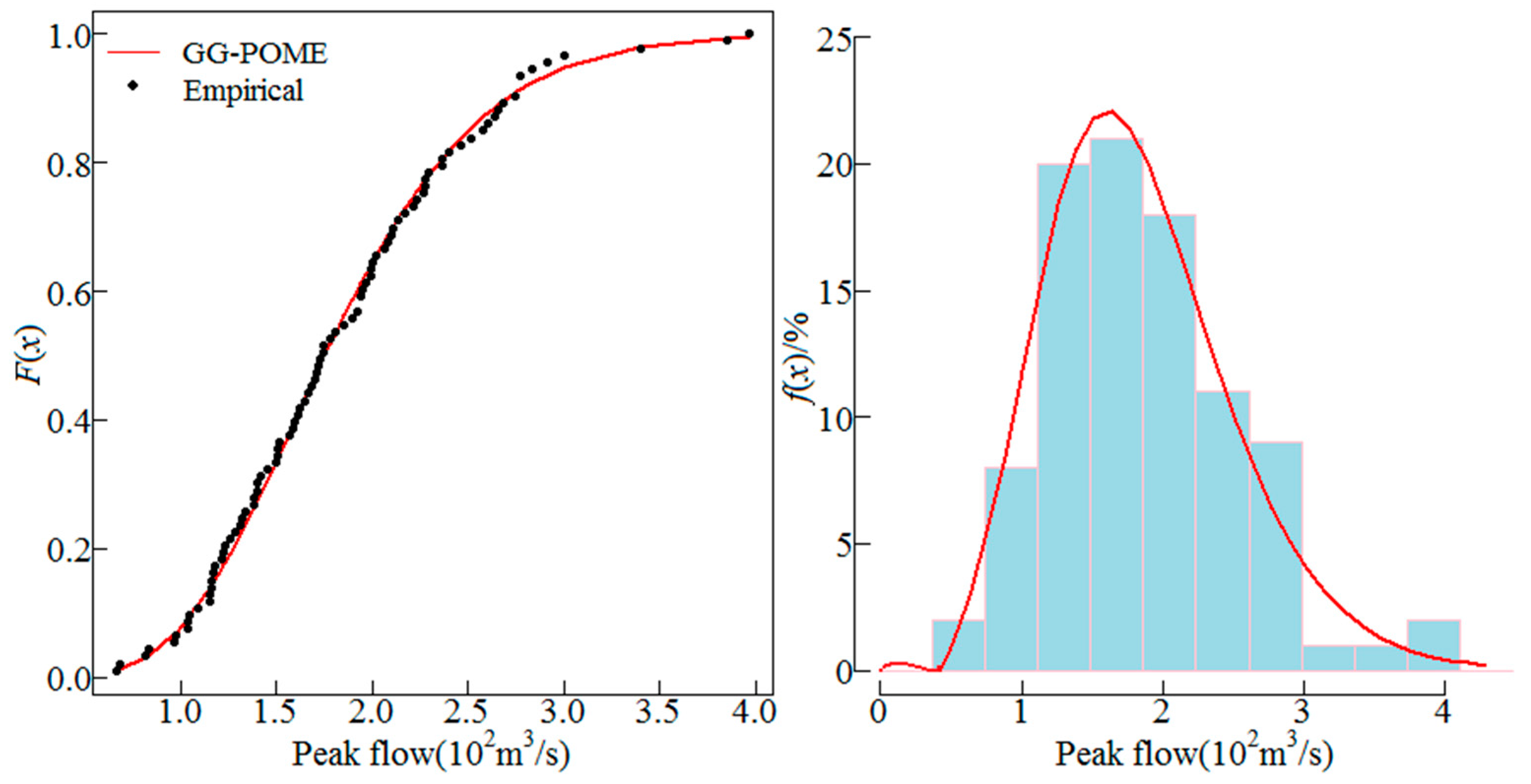
Besides AM series, partial-duration series can be also employed for the POME method. In this study, the AM series was considered since it is more widely used. The GG distribution was employed to fit the AM series of the 10 sites. The distribution parameters were estimated using Equations (16). The fitted GG distribution and the empirical frequency distribution of the AM series from sites 1, 5, 6 and 8 are shown in Figure 2, Figure 3, Figure 4 and Figure 5. These four sites are selected because sites 5 and 8 have low skews, site 1 has moderate skew and site 6 has high skew, the cumulative distributions and histograms of AM series fitted by GG distribution for these sites can be representative. The line represents the fitted distribution and point represents the empirical frequencies of observations. Results show that the GG distribution fitted the empirical data well. Histograms of the AM flood peak series fitted by the GG distribution for the four sites are also shown in Figure 2, Figure 3, Figure 4 and Figure 5 which also show that the GG distribution fitted the empirical histograms well. The skewness coefficient of AM series of sites 1, 5, 6 and 8 was 1.94, 0.66, 2.93 and 0.75, respectively, which showed that the GG distribution described both low and high skewed data well.
Several distributions, including normal (NM), exponential (EXP), generalized logistic (GLO), gamma (GM), generalized Pareto (GPA), Gumbel (GB), Weibull (WB), P3, GEV and LP3 distributions, in which the parameters of EXP, GLO, GM, GPA, GB, WB, P3, GEV distributions were estimated by the L-moment method (LM) [11,17], while the parameters of NM and LP3 distributions were estimated by MM [18,19]. These FFA models were also fitted to the AM series for the 10 sites and the values of RMSE and AIC were computed for each model using Equations (17) and (18) and listed in Table 2.
where n denotes the sample size, K is the number of parameters of the distribution, is the theoretical non-exceedance probability calculated by the distribution, and P is the empirical non-exceedance probability. Root mean square error (RMSE) is a frequently used measure of the differences between values (sample and population values) predicted by a model or an estimator and the values actually observed. The smaller RMSE values represent the better performance of the model. The Akaike information criterion (AIC) is a measure of the relative quality of statistical models for a given set of data. It also includes a penalty that is an increasing function of the number of estimated parameters. Given a set of candidate models for the data, the preferred model is the one with the minimum AIC value.
Table 2 illustrates that for sites 1, 2, 4, 5, 8, 9 and 10, the GG distribution had the smallest RMSE values, which means the GG distribution fitted the observed AM data best. In addition, the GG distribution had the smallest AIC values for sites 2, 5, 8, and 10. Table 2 also indicates that the average RMSE and AIC values of GG distribution are the smallest among all the compared distributions. Thus, the GG distribution performs better than other distributions.
Table 2 also shows that the GG, P3, GEV, LP3 distributions gave quite similar performances for most of the selected sites. However, it was observed that the GG distribution performed better at several sites. For site 2, the RMSE values for the GG, P3, and GEV distributions were 0.028, 0.033 and 0.034, respectively. The AIC values were −417.67, −351.64 and −347.79, respectively. Thus, the GG distribution performed much better than the P3 and GEV distributions for site 2. Compared with the LP3 distribution, the GG distribution was more appropriate for sites 5 and 7. For site 5, the RMSE and AIC values for the LP3 distribution (GG distribution) were 0.016(0.013) and −559.41 (−578.63), respectively. For site 7, the RMSE and AIC values for the LP3 distribution (GG distribution) were 0.019(0.016) and −545.85 (−571.71), respectively. Thus, the GG distribution outperformed the LP3 distribution for those two sites. The above discussions shows that the GG distribution is either superior or comparable to the commonly used distributions.
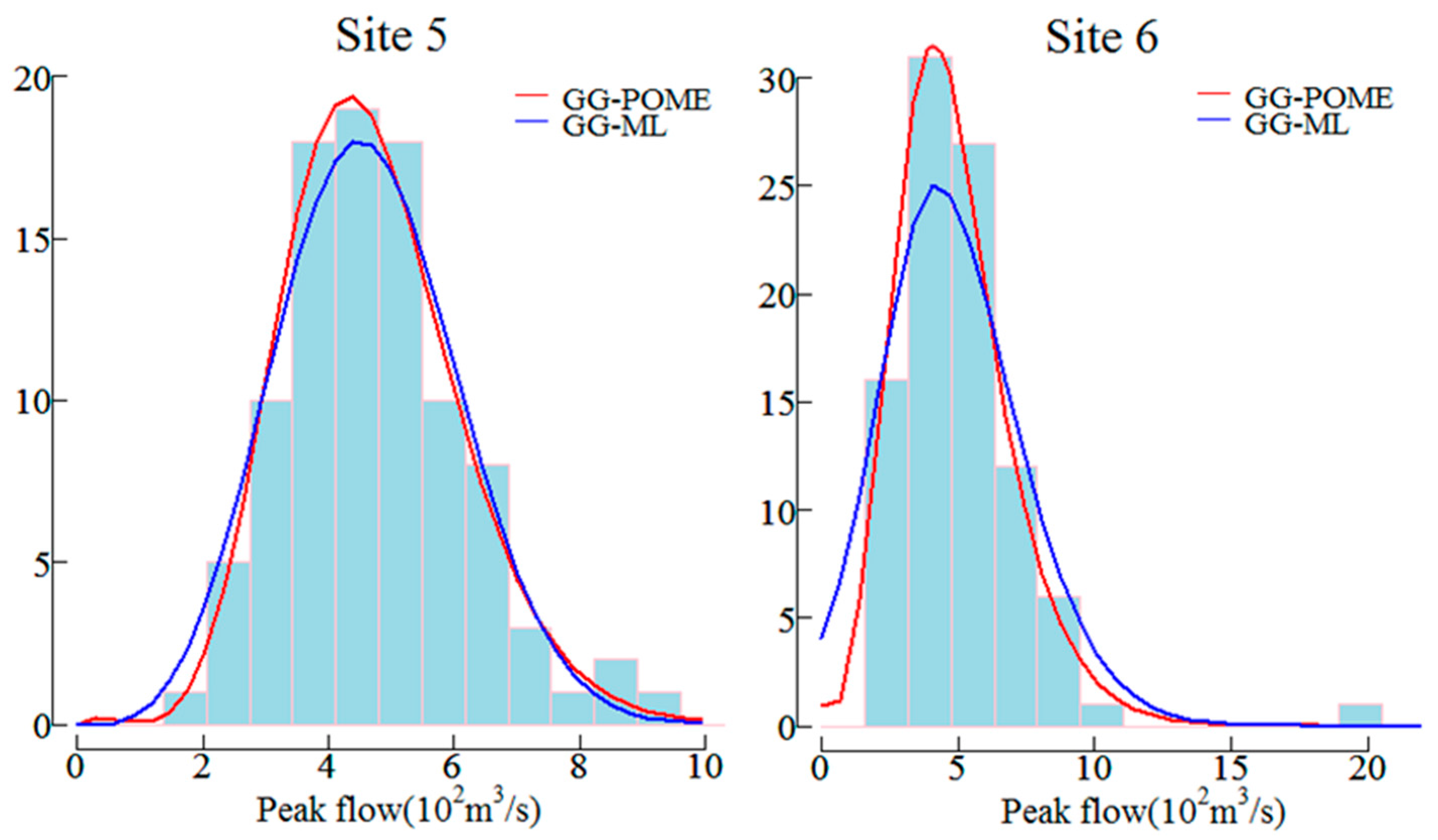
The maximum likelihood (ML) method was also employed for GG distribution and compared with the proposed GG-POME model for site 5 (low skew) and site 6 (high skew). Figure 6 gives comparisons of their probability density functions and indicates that the GG-POME model gives a better performance. The RMSE and AIC values of GG-ML model for sites 5 and 6 were also calculated. The RMSE and AIC values for the GG-ML (GG-POME) model are 0.023 (0.013) and −497.54 (−578.63), respectively for site 5. And the RMSE and AIC values for the GG-ML (GG-POME) model are 0.032 (0.024) and −379.24 (−427.53), respectively for site 6. Therefore it may imply that GG-POME model outperforms GG-ML model.
4. Monte Carlo Simulation
The predictive ability of the GG distribution was evaluated using Monte Carlo simulation and compared with that of the P3, GEV, and LP3 distributions. To test how well a candidate distribution estimated the magnitude-return period relationship, a parent distribution which was not identical to any of the candidate distributions was chosen. Cunnane [20] recommended that such a parent distribution should be a Wakeby distribution with certain parameters. In this study, three kinds of data sets were generated from the Wakeby distribution with parameters as shown in Table 3. The Wakeby distribution has quantile function given as [21]:
where F is the uniform (0, 1) variate; and are the parameters.
Then, the real quantile value QT was computed. S = 1000 samples with size n (n = 20, 50, 100) were generated from each Wakeby distribution and fitted by the four distributions to estimate the events of T = 10, 100 and 1000-year return periods. Table 4 lists the RB and RRMSE values computed by each distribution using Equations (20) and (21):
where QT is a given parent quantile, are the estimators for the samples generated from the Wakeby distribution, and S is the number of Monte Carlo trials. The relative bias (RB) and the relative root mean square errors (RRMSE) were used to evaluate the accuracy and efficiency of a candidate model, respectively.
From Table 4, generally for all distributions and for all cases, it was observed that the RB and RRMSE values increased with the return period T. For a small return period (T = 10), the selected four distributions exhibited very similar behaviors regardless of the sample size. For moderate and large return periods (T = 100 and 1000), notable differences of RB and RRMSE values were observed. Thus, in the latter discussion, we would mainly focus on moderate and high return period quantile estimators.
For case 1 (Cv = 0.2, Cs = 0.16), it was observed that the GG and P3 distributions were superior to the GEV and LP3 distributions. When the sample size equaled 100 or 50, the P3 distribution quantile estimators had the smallest RB values for both moderate and large return periods (T = 100 and 1000). But the GG distribution quantile estimators had smaller RRMSE values for T = 1000 than other distributions. For a small sample size (n = 20), the GG distribution had the smallest RB and RRMSE values for both moderate and large return periods (T = 100 and 1000). For T = 1000, the RRMSE values of the GG, P3, GEV and LP3 distributions were 6.46, 9.08, 10.84 and 10.03, respectively. Apparently, the GG distribution performed much better when the sample size was small. This indicates that the GG distribution was more robust. Thus, for case 1, the P3 distribution was preferable when the sample size was large than 50, while the GG distribution was more appropriate when sample size did not exceed 50.
For case 2 (Cv = 0.36, Cs = 0.48), results indicated that for sample size n = 50 and n = 100, the GEV distribution quantile estimators had the smallest RB values for T = 100 and the LP3 distribution quantile estimators had the smallest RB values for T = 1000. However, their RRMSE values were quite large and increased significantly when the sample sizes decreased. For T = 1000, when the sample size decreased from 100 to 20, the RRMSE values of the GEV distribution rose from 16.35 to 34.45, and the RRMSE values of the LP3 distribution rose from 13.51 to 44.85. While the RRMSE values of the GG distribution rose slightly from 4.8 to 14.18. This was due to the poor accuracy of the GEV and LP3 distributions parameter estimators which had high variance for small sample sizes. In this case, the GG distribution performed significantly better than the other three distributions. Its RB values were quite small, and its RRMSE values were the smallest for all sample sizes and return periods. This was a good indication of the robustness of the GG distribution for this case.
For case 3 (Cv = 0.55, Cs = 0.97), all distribution quantile estimators had quite large RB and RRMSE values. For n = 50 and n = 100, RB and RRMSE of the GEV distribution were the highest, which amounted to 21.02 and 33.68, respectively, for n = 50, T = 1000, while the GG distribution yielded 16.86 and 22.85, respectively. Also for n = 50 and n = 100, the LP3 distribution quantile estimators had the smallest RB values for both T = 100 and T = 1000, and the other three distributions had similar RB values. But the LP3 distribution gave the worst performance for small sample sizes (n = 20). Its RB and RRMSE values were 26.58 and 57.28, respectively, for T = 1000, whereas the GG distribution yielded 17.67 and 28.16, respectively. In this case, the RB values of the GG distribution were comparable to the P3 and GEV distributions, and were a little larger than the LP3 distribution for n = 50 and n = 100, the RRMSE values of the GG distribution were the smallest for both moderate and large return periods (T = 100 and 1000) regardless of the sample size. Also, when the sample size decreased from 100 to 20, the RB and RRMSE values of the GG distribution rose from 17.52 and 19.32 to 17.67 and 28.16, respectively. This might imply that the distribution was less affected by sample size. Thus, the GG distribution was superior to other distributions for this case. Therefore, the predictive ability of the GG distribution was found to be comparable or superior to that of the other distributions, and it was more robust since it was less affected by sample size, and therefore, estimated the magnitude-return period relationships better.
5. T-Year Design Flood Calculation
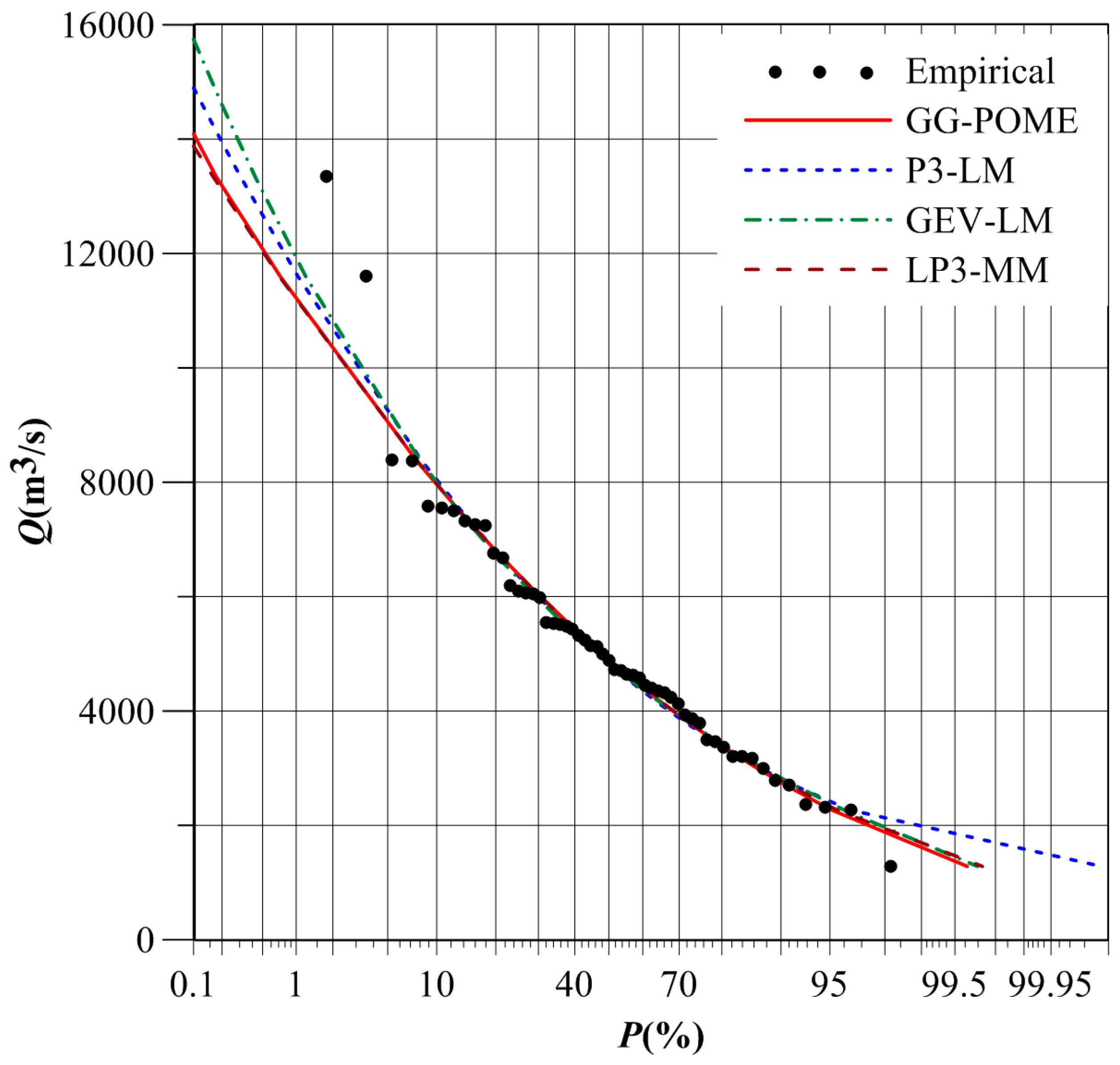
The Danjiangkou reservoir lies in the upper Hanjiang basin and is the source of water for the Middle Route Project under the South-to-North Water Transfer Scheme in China [22]. The Geheyan reservoir, with a volume of 3.12 billion m3, plays an important role in management of Qingjiang River [23]. Flood frequency analysis for these two sites was therefore considered in this study. The T-year design flood calculated by different FFA distributions at Danjiangkou Reservoir and Geheyan Reservoir are listed in Table 5. Figure 7 and Figure 8 compare frequency curves of different distributions at these two reservoir sites.
Table 5 indicates that design flood for small return periods was similar for these four distributions. However, significant differences were observed for large return periods. The 1000-year design flood calculated by the GG and LP3 distributions at Danjiangkou Reservoir were 55,234 m3/s and 48,822 m3/s, respectively. And the 1000-year design flood calculated by the GEV and LP3 distributions at Geheyan Reservoir were 15,746 m3/s and 13,877 m3/s, respectively.
Figure 7 indicates that the GG, P3, and GEV distributions had quite similar flood quantile estimators for large return periods at Danjiangkou Reservoir. However, the 1000-year design flood calculated by the LP3 distribution was smaller than by the other three distributions. Figure 8 indicates that the 1000-year design flood calculated by the GEV distribution at Geheyan Reservoir was the largest, and was the smallest for the LP3 distribution.
The design flood calculated by the GG distribution was quite close to that by the LP3 distribution. Besides, the P3 distribution has been adopted in China as a uniform procedure for FFA [24,25]. Table 2 shows that RMSE and AIC values for the P3 distribution at Danjiangkou Reservoir were 0.023 and −419.04, respectively, and the GG distribution yielded 0.021 and −421.51, respectively. The RMSE and AIC values for the P3 distribution at Geheyan Reservoir were 0.027 and −249.79, respectively, and the GG distribution yielded 0.023 and −269.84, respectively. Thus, the performance of the GG distribution was better than that of the P3 distribution. Therefore, the design flood estimated by the GG distribution would be preferable in practice.
6. Conclusions
In this study, the GG distribution with parameters estimated by POME was applied for FFA. Ten gauging stations were selected as a case study to test the GG distribution. Frequency estimates from the GG distribution were also compared with those of commonly used distributions. A Monte Carlo simulation study was carried out to evaluate the predictive ability of the GG distribution and compare it with other distributions. In addition, some characteristics of frequency curves at Danjiangkou Reservoir and Geheyan Reservoir were evaluated. The following conclusions are drawn from this study:
- (1)
- The GG distribution is appealing for FFA. The cumulative distributions and histograms show that the GG distribution can fit both low and high skewed data well.
- (2)
- The parameters estimated by POME are found reasonable. Both the marginal distributions and histograms indicates that the GG distribution with so estimated parameters can successfully be fitted to empirical values.
- (3)
- The performance of the GG distribution is comparable or superior to that of the other distributions. Results illustrate that for sites 1, 2, 4, 5, 8, 9 and 10, the GG distribution has the smallest RMSE values. In addition, the GG distribution has the smallest AIC values for sites 2, 5, 8, and 10. Thus, the GG distribution is preferred to other distributions for those sites. Furthermore, the GG, P3, GEV, and LP3 distributions give similar performance for most of the selected sites. However, the GG distribution fits better than them for a few sites.
- (4)
- The predictive ability of the GG distribution is found to be comparable or superior to widely accepted distributions. The GG distribution performs significantly better than the other three distributions when sample sizes are small. Thus it is less effected by sample size and is more robust.
Acknowledgments
This study was supported by the National Natural Science Foundation of China (51679094; 51509273; 91547208) and Fundamental Research Funds for the Central Universities (2016YXZD048).
Author Contributions
All of the authors read and approved the final manuscript. Lu Chen and Feng Xiong conceived and designed the experiments; Vijay P. Singh analyzed the data and contributed materials; Lu Chen and Feng Xiong wrote the paper.
Conflicts of Interest
The authors declare no conflict of interest.
References
- American Society of Civil Engineers. Hydrology Handbook, 2nd ed.; ACSE: New York, NY, USA, 1996. [Google Scholar]
- Chen, L.; Guo, S.; Yan, B.; Liu, P.; Fang, B. A new seasonal design flood method based on bivariate joint distribution of flood magnitude and date of occurrence. Hydrol. Sci. J. 2010, 55, 1264–1280. [Google Scholar] [CrossRef]
- Chen, L.; Singh, V.P.; Guo, S.; Hao, Z.; Li, T. Flood coincidence risk analysis using multivariate copula functions. J. Hydrol. Eng. 2012, 17, 742–755. [Google Scholar] [CrossRef]
- Kasiviswanathan, K.S.; He, J.X.; Tay, J.H. Flood frequency analysis using multi-objective optimization based interval estimation approach. J. Hydrol. 2017, 545, 251–262. [Google Scholar] [CrossRef]
- Chen, L.; Singh, V.P.; Guo, S.; Zhou, J.; Zhang, J. Copula-based method for multisite monthly and daily streamflow simulation. J. Hydrol. 2015, 528, 369–384. [Google Scholar] [CrossRef]
- Benameur, S.; Benkhaled, A.; Meraghni, D.; Chebana, F.; Necir, A. Complete flood frequency analysis in Abiod watershed, Biskra (Algeria). Nat. Hazards 2017, 86, 519–534. [Google Scholar] [CrossRef]
- Natural Environment Research Council. Flood Studies Report; Institute of Hydrology: London, UK, 1975. [Google Scholar]
- Natural Environment Research Council. Flood Studies Report; Institute of Hydrology: Wallingford, UK, 1999. [Google Scholar]
- Papalexiou, S.M.; Koutsoyiannis, D. Entropy based derivation of probability distributions: A case study to daily rainfall. Adv. Water Resour. 2012, 45, 51–57. [Google Scholar] [CrossRef]
- Chebana, F.; Adlouni, S.; Bobée, B. Mixed estimation methods for Halphen distributions with applications in extreme hydrologic events. Stoch. Environ. Res. Risk. Assess. 2010, 24, 359–376. [Google Scholar] [CrossRef]
- Hosking, J.R.M. L-moments: analysis and estimation of distributions using linear combinations of order statistics. J. R. Stat. Soc. 1990, 52, 105–124. [Google Scholar]
- Singh, V.P. Entropy-Based Parameter Estimation in Hydrology; Springer: Dordrecht, The Netherlands, 1998. [Google Scholar]
- Shannon, C.E. A mathematical theory of communication. Bell Syst. Tech. J. 1948, 27, 379–423. [Google Scholar] [CrossRef]
- Singh, V.P. Entropy Theory and Its Application in Environmental and Water Engineering; John Wiley & Sons: Chichester, UK, 2013. [Google Scholar]
- Singh, V.P. Entropy Theory in Hydrologic Science and Engineering; McGraw-Hill Education: New York, NY, USA, 2014. [Google Scholar]
- Deuflhard, P. Newton Methods for Nonlinear Problems: Affine Invariance and Adaptive Algorithms; Springer: Berlin, Germany, 2011. [Google Scholar]
- Liang, Z.; Hu, Y.; Li, B.; Yu, Z. A modified weighted function method for parameter estimation of Pearson type three distribution. Water Resour. Res. 2014, 50, 3216–3228. [Google Scholar] [CrossRef]
- Rao, A.R.; Hamed, K.H. Flood Frequency Analysis; CRC Press: New York, NY, USA, 2000. [Google Scholar]
- Griffis, V.W.; Stedinger, J.R. Log-Pearson type 3 distribution and its application in flood frequency analysis. II: Parameter estimation methods. J. Hydrol. Eng. 2007, 12, 482–491. [Google Scholar] [CrossRef]
- Cunnane, C. Statistical distribution for flood frequency analysis. Oper. Hydrol. Rep. 1989, 44, 369. [Google Scholar]
- Houghton, J.C. Birth of a parent: The Wakeby distribution for modeling flood flows. Water Resour. Res. 1978, 14, 1105–1109. [Google Scholar] [CrossRef]
- Li, S.; Xu, Z.; Cheng, X.; Zhang, Q. Dissolved trace elements and heavy metals in the Danjiangkou Reservoir, China. Environ. Geol. 2008, 55, 977–983. [Google Scholar] [CrossRef]
- Qi, S.; Yan, F.; Wang, S.; Xu, R. Characteristics, mechanism and development tendency of deformation of Maoping landslide after commission of Geheyan reservoir on the Qingjiang River, Hubei Province, China. Eng. Geol. 2006, 86, 37–51. [Google Scholar] [CrossRef]
- Ji, X.; Ding, J.; Shen, H.; Salas, J.D. Plotting positions for Pearson type-III distribution. J. Hydrol. 1984, 74, 1–29. [Google Scholar]
- Shao, Q.; Wong, H.; Xia, J.; Ip, W. Models for extremes using the extended three-parameter Burr XII system with application to flood frequency analysis. Hydrol. Sci. J. 2004, 49, 685–702. [Google Scholar] [CrossRef]
Figure 1.
Flow chart of POME method for parameter estimation.
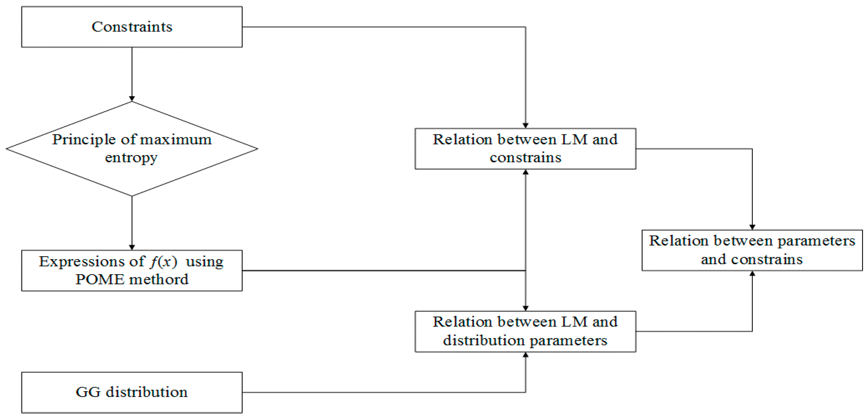
Figure 2.
Cumulative distribution and histogram of AM flood peak series fitted by the GG distribution for site 1.
Figure 2.
Cumulative distribution and histogram of AM flood peak series fitted by the GG distribution for site 1.

Figure 3.
Cumulative distribution and histogram of AM flood peak series fitted by the GG distribution for site 5.
Figure 3.
Cumulative distribution and histogram of AM flood peak series fitted by the GG distribution for site 5.

Figure 4.
Cumulative distribution and histogram of AM flood peak series fitted by GG-POME model for site 6.
Figure 4.
Cumulative distribution and histogram of AM flood peak series fitted by GG-POME model for site 6.

Figure 5.
Cumulative distribution and histogram of AM flood peak series fitted by the GG distribution for site 8.
Figure 5.
Cumulative distribution and histogram of AM flood peak series fitted by the GG distribution for site 8.

Figure 6.
Comparisons of probability density functions of GG-POME and GG-ML models for sites 5 and 6.
Figure 6.
Comparisons of probability density functions of GG-POME and GG-ML models for sites 5 and 6.

Figure 7.
Frequency curves of different FFA distributions at Danjiangkou Reservoir.
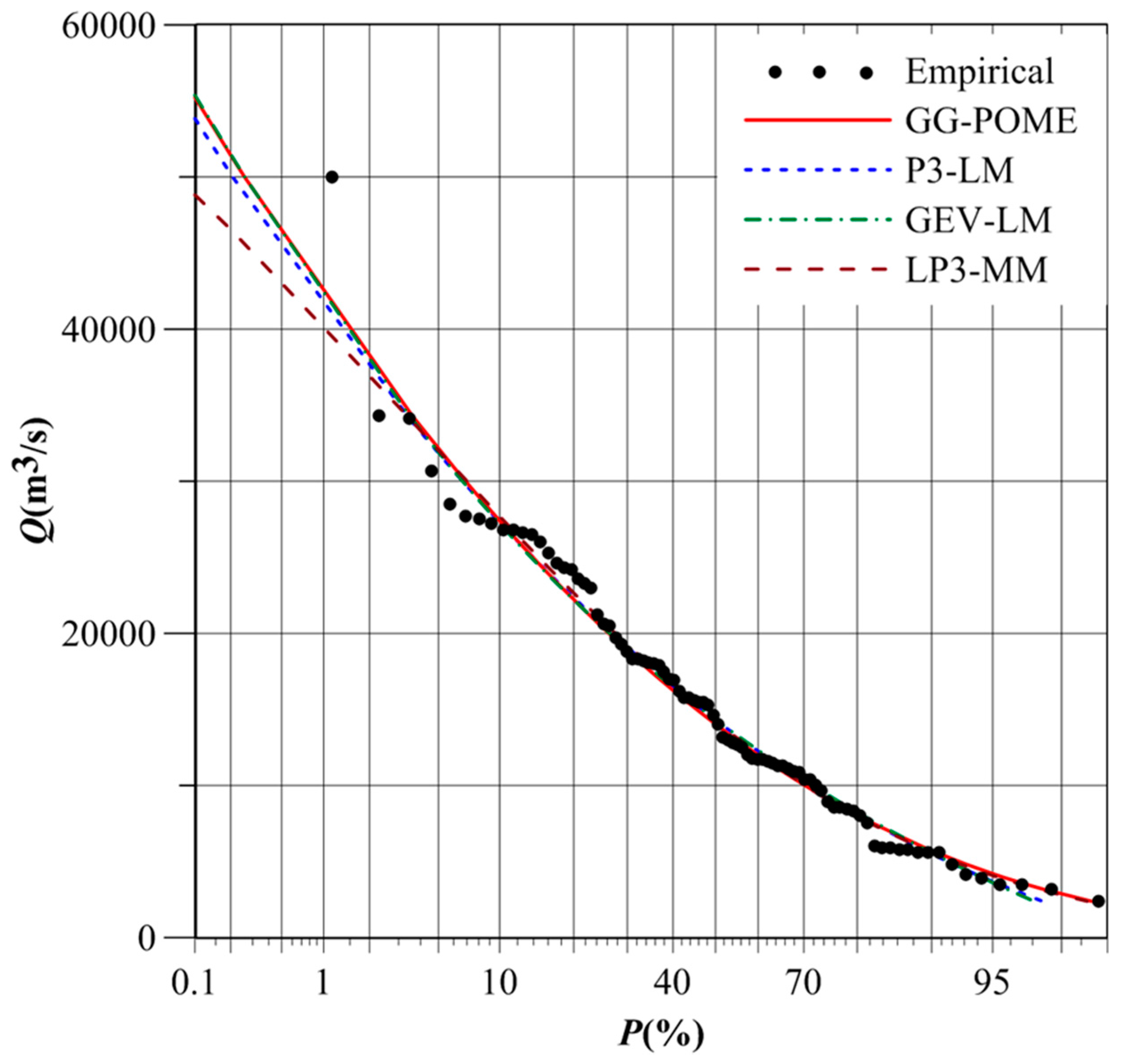
Figure 8.
Frequency curves of different FFA distributions at Geheyan Reservoir.

Table 1.
Statistics of annual maximum flood data series for 10 sites.
| Site No. | Gauging Station | Period | Cv | Cs | Ck |
|---|---|---|---|---|---|
| 1 | Rogue River at Raygold near Central Point, US | 1906–2001 | 0.67 | 1.94 | 5.66 |
| 2 | Quinault River at Quinault Lake, US | 1912–2001 | 0.40 | 0.52 | −0.6 |
| 3 | Eel R A Scotla, US | 1911–2001 | 0.51 | 0.61 | −0.44 |
| 4 | White River Near Meeker, US | 1910–2001 | 0.34 | 0.65 | 0.77 |
| 5 | Yellowstone River at Corwin Springs, US | 1890–2001 | 0.30 | 0.66 | 0.59 |
| 6 | Genesee River at Portageville, US | 1909–2001 | 0.48 | 2.93 | 15.67 |
| 7 | White River Near Meeker, US | 1910–2001 | 0.34 | 0.65 | 0.77 |
| 8 | Brokenstraw Creek at Younsville, US | 1910–2001 | 0.33 | 0.75 | 0.65 |
| 9 | Danjiangkou reservior at Danjiangkou, China | 1929–2014 | 0.56 | 0.95 | 1.57 |
| 10 | Geheyan reservior at Changyang, China | 1951–2005 | 0.42 | 1.34 | 3.34 |
Table 2.
The RMSE and AIC values of different flood frequency analysis distributions.
| Model | Site 1 | Site 2 | Site 3 | Site 4 | Site 5 | Mean Value | |||||
| RMSE | AIC | RMSE | AIC | RMSE | AIC | RMSE | AIC | RMSE | AIC | RMSE | |
| GG-POME | 0.016 | −508.12 | 0.028 | −417.67 | 0.023 | −430.63 | 0.021 | −462.6 | 0.013 | −578.63 | 0.020 |
| NM-MM | 0.078 | −258.88 | 0.047 | −306.32 | 0.048 | −316.43 | 0.037 | −394.91 | 0.038 | −407.87 | 0.053 |
| EXP-LM | 0.021 | −468.96 | 0.056 | −273.3 | 0.054 | −218.65 | 0.069 | −244.39 | 0.058 | −286.44 | 0.054 |
| GLO-LM | 0.025 | −446.68 | 0.046 | −303.81 | 0.035 | −362.47 | 0.021 | −474.16 | 0.015 | −560.19 | 0.027 |
| GM-LM | 0.029 | −447.1 | 0.032 | −362.45 | 0.021 | −447.48 | 0.021 | −467.06 | 0.017 | −550.61 | 0.027 |
| GPA-LM | 0.019 | −504.1 | 0.029 | −413.67 | 0.021 | −444.15 | 0.042 | −346.33 | 0.036 | −389.21 | 0.030 |
| GB-LM | 0.039 | −386.64 | 0.036 | −343.98 | 0.025 | −421.83 | 0.024 | −430.95 | 0.015 | −530.05 | 0.031 |
| WB-LM | 0.017 | −522.29 | 0.029 | −372.34 | 0.019 | −459.48 | 0.025 | −441.45 | 0.019 | −515.48 | 0.024 |
| P3-LM | 0.016 | −533.04 | 0.033 | −351.64 | 0.023 | −434.97 | 0.021 | −468.95 | 0.015 | −561.44 | 0.024 |
| GEV-LM | 0.019 | −495.44 | 0.034 | −347.79 | 0.025 | −419.06 | 0.021 | −472.43 | 0.014 | −572.29 | 0.022 |
| LP3-MM | 0.016 | −528.15 | 0.028 | −376.18 | 0.021 | −450.45 | 0.024 | −451.6 | 0.016 | −559.41 | 0.021 |
| Site 6 | Site 7 | Site 8 | Site 9 | Site 10 | Mean Value | ||||||
| RMSE | AIC | RMSE | AIC | RMSE | AIC | RMSE | AIC | RMSE | AIC | AIC | |
| GG-POME | 0.024 | −427.53 | 0.021 | −447.25 | 0.013 | −562.19 | 0.021 | −421.51 | 0.023 | −269.84 | −452.60 |
| NM-MM | 0.038 | −407.87 | 0.113 | −198.3 | 0.035 | −400.26 | 0.046 | −313.47 | 0.051 | −210.33 | −321.46 |
| EXP-LM | 0.058 | −286.44 | 0.04 | −373.78 | 0.059 | −271.25 | 0.064 | −233.3 | 0.061 | −150.65 | −280.72 |
| GLO-LM | 0.033 | −377.21 | 0.014 | −520.86 | 0.023 | −449.16 | 0.031 | −368.25 | 0.023 | −267.35 | −413.01 |
| GM-LM | 0.038 | −393.42 | 0.046 | −374.75 | 0.014 | −541.17 | 0.023 | −404.7 | 0.027 | −264.86 | −425.36 |
| GPA-LM | 0.024 | −444.17 | 0.032 | −359.81 | 0.025 | −464.21 | 0.027 | −384.59 | 0.044 | −194.88 | −394.51 |
| GB-LM | 0.033 | −404.93 | 0.072 | −282.68 | 0.019 | −475.75 | 0.024 | −406.35 | 0.024 | −262.96 | −394.61 |
| WB-LM | 0.022 | −454.57 | 0.042 | −312.87 | 0.013 | −559.08 | 0.021 | −429.65 | 0.030 | −237.83 | −430.50 |
| P3-LM | 0.022 | −452.78 | 0.051 | −275.86 | 0.014 | −538.15 | 0.023 | −419.04 | 0.027 | −249.79 | −428.57 |
| GEV-LM | 0.027 | −411.21 | 0.021 | −438.69 | 0.015 | −525.05 | 0.024 | −409.68 | 0.024 | −260.26 | −435.19 |
| LP3-MM | 0.026 | −418.17 | 0.022 | −450.08 | 0.014 | −536.12 | 0.021 | −426.08 | 0.026 | −262.16 | −445.84 |
Table 3.
Monte Carlo simulation data sets generated from the Wakeby distribution.
| ξ | α | β | γ | δ | Cv | Cs | |
|---|---|---|---|---|---|---|---|
| Case 1 | 30.4 | 114.2 | 11.3 | 19.2 | −0.5 | 0.2 | 0.16 |
| Case 2 | 15.4 | 308.8 | 10.25 | 38.5 | −0.3 | 0.36 | 0.48 |
| Case 3 | 23.5 | 198.6 | 3.7 | 109.2 | −0.2 | 0.55 | 0.95 |
Table 4.
Calculated RB and RRMSE values for different FFA distributions.
| GG-POME | P3-LM | GEV-LM | LP3-MM | |||||||
|---|---|---|---|---|---|---|---|---|---|---|
| RB | RRMSE | RB | RRMSE | RB | RRMSE | RB | RRMSE | |||
| T = 10 | −1.71 | 4.54 | −1.21 | 3.64 | −0.87 | 3.78 | −0.89 | 4.07 | ||
| n = 20 | T = 100 | 6.11 | 7.95 | 4.6 | 9.26 | 4.89 | 9.31 | 2.56 | 8.84 | |
| T = 1000 | 2.02 | 6.46 | 2.29 | 9.08 | 5.11 | 10.84 | 4.15 | 10.03 | ||
| T = 10 | −1.32 | 2.73 | −0.87 | 2.45 | −0.75 | 2.43 | −0.81 | 2.48 | ||
| Case 1 | n = 50 | T = 100 | 5.53 | 6.5 | 4.38 | 6.28 | 6.12 | 8.02 | 4.25 | 6.77 |
| T = 1000 | 1.85 | 4.9 | 0.02 | 6.73 | 2.87 | 8.1 | 0.65 | 7.31 | ||
| T = 10 | −1.06 | 1.82 | −1.05 | 1.86 | −0.72 | 1.84 | −0.71 | 1.82 | ||
| n = 100 | T = 100 | 6.02 | 6.55 | 4.97 | 5.72 | 5.47 | 6.34 | 4.74 | 5.82 | |
| T = 1000 | 1.46 | 3.42 | 0.21 | 4.29 | 2.93 | 6.03 | 0.55 | 5.46 | ||
| T = 10 | −2.65 | 9.78 | −0.82 | 9.78 | −0.58 | 9.34 | −0.35 | 14.78 | ||
| n = 20 | T = 100 | 1.93 | 10.23 | 2.25 | 16.85 | 3.64 | 19.23 | 5.97 | 39.86 | |
| T = 1000 | 3.59 | 14.18 | 8.69 | 24.29 | 16.48 | 34.45 | 11.62 | 44.85 | ||
| T = 10 | −1.93 | 8.44 | −1.57 | 6.76 | −1.76 | 6.21 | −1.26 | 6.63 | ||
| Case 2 | n = 50 | T = 100 | 1.66 | 7.55 | 1.76 | 10.27 | 1.37 | 10.74 | −1.67 | 12.54 |
| T = 1000 | 3.27 | 10.33 | 8.64 | 16.46 | 6.67 | 18.96 | 4.32 | 21.43 | ||
| T = 10 | −1.21 | 5.86 | −1.18 | 4.73 | −0.58 | 4.34 | −0.86 | 4.52 | ||
| n = 100 | T = 100 | 1.94 | 5.87 | 1.37 | 6.24 | 0.87 | 7.52 | −1.24 | 7.88 | |
| T = 1000 | 4.22 | 8.4 | 9.49 | 12.78 | 8.72 | 16.35 | 0.29 | 13.51 | ||
| T = 10 | −0.42 | 11.46 | −0.58 | 13.43 | −2.34 | 12.57 | 2.64 | 14.79 | ||
| n = 20 | T = 100 | 5.1 | 14 | 7.86 | 21.95 | 8.54 | 23.35 | 4.96 | 31.38 | |
| T = 1000 | 17.67 | 28.16 | 13.57 | 29.87 | 21.82 | 42.72 | 26.58 | 57.28 | ||
| T = 10 | -0.41 | 8.78 | 0.86 | 7.96 | −1.25 | 7.38 | 1.78 | 8.67 | ||
| Case 3 | n = 50 | T = 100 | 6.34 | 12.38 | 4.62 | 13.94 | 6.44 | 15.86 | 4.41 | 16.34 |
| T = 1000 | 16.86 | 22.85 | 14.53 | 24.63 | 21.02 | 33.68 | 8.29 | 27.32 | ||
| T = 10 | −0.42 | 5.72 | −0.87 | 5.87 | −1.15 | 5.46 | 0.26 | 5.74 | ||
| n = 100 | T = 100 | 6.37 | 8.54 | 4.75 | 8.98 | 6.65 | 11.87 | 3.54 | 12.64 | |
| T = 1000 | 17.52 | 19.32 | 15.67 | 19.78 | 17.98 | 23.92 | 7.66 | 20.67 | ||
Table 5.
Comparison of T-year design floods calculated by different FFA distributions at Danjiangkou and Geheyan sites.
Table 5.
Comparison of T-year design floods calculated by different FFA distributions at Danjiangkou and Geheyan sites.
| Site | Model | Return Period (Year) | ||||
|---|---|---|---|---|---|---|
| 1000 | 500 | 100 | 50 | 10 | ||
| GG-POME | 55,234 | 51,432 | 42,204 | 38,803 | 27,398 | |
| Danjiangkou | P3-LM | 53,838 | 50,202 | 41,407 | 37,411 | 27,311 |
| (m3/s) | GEV-LM | 55,369 | 51,490 | 42,054 | 37,785 | 27,217 |
| LP3-MM | 48,822 | 46,561 | 40,261 | 36,999 | 27,692 | |
| GG-POME | 13,992 | 13,745 | 11,186 | 10,277 | 7957 | |
| Geheyan | P3-LM | 14,896 | 13,941 | 11,648 | 10,616 | 8039 |
| (m3/s) | GEV-LM | 15,746 | 14,594 | 11,910 | 10,746 | 7991 |
| LP3-MM | 13,877 | 13,099 | 11,171 | 10,276 | 7963 | |
© 2017 by the authors. Licensee MDPI, Basel, Switzerland. This article is an open access article distributed under the terms and conditions of the Creative Commons Attribution (CC BY) license (http://creativecommons.org/licenses/by/4.0/).
Share and Cite
MDPI and ACS Style
Chen, L.; Singh, V.P.; Xiong, F. An Entropy-Based Generalized Gamma Distribution for Flood Frequency Analysis. Entropy 2017, 19, 239. https://doi.org/10.3390/e19060239
AMA Style
Chen L, Singh VP, Xiong F. An Entropy-Based Generalized Gamma Distribution for Flood Frequency Analysis. Entropy. 2017; 19(6):239. https://doi.org/10.3390/e19060239
Chicago/Turabian StyleChen, Lu, Vijay P. Singh, and Feng Xiong. 2017. "An Entropy-Based Generalized Gamma Distribution for Flood Frequency Analysis" Entropy 19, no. 6: 239. https://doi.org/10.3390/e19060239
Note that from the first issue of 2016, this journal uses article numbers instead of page numbers. See further details here.