1. Introduction
The generation of optimal simulation input points is of particular interest for long running computer codes. As in the field of plasma–wall interactions of fusion plasmas, the running time of the simulation codes is in the order of months, so the input parameter settings should better be chosen well. Though considerable parallelization efforts have been spent to accelerate the code, the speed-up is limited to a certain margin, from which point on it is futile to utilize more and more processor cores. Apart from this drawback, one would still have to wait for a sequential execution of one parameter setting after the other, since the next best set of input parameters depends on the previous result. This paper overcomes this by proposing several most promising parameter setups which are obtained by marginalizing over optimal input points. The pool of such independent starting sets enables the parallel execution of the original simulation code.
The problem of predicting function values in a multi-dimensional space supported by given data is a regression problem for a non-trivial function of unknown shape. Given
n input data vectors
of dimension
(with matrix
) and corresponding target data
blurred by Gaussian noise of variance
, the sought quantity is the target value
at test input vector
. The latter would be generated by a function
where
and
. Since we are completely ignorant about a model describing function, our ansatz is to employ the Gaussian process method, with which any uniformly continuous function may be represented. As a statistical process, it is fully defined by its covariance function and called Gaussian, because any collection of random variables produced by this process has a Gaussian distribution.
The Gaussian process method defines a distribution over functions. One can think of the analysis as taking place in a space of functions (function-space view), which is conceptually different from the familiar view of solving the regression problem of, for instance, the standard linear model (SLM)
in the space of the weights
(weight-space view). At this point, it is instructive to restate the results for the latter: the predictive distribution depending on mean
and variance for a test input data point
is given by
with
is the covariance in a Gaussian prior on the weights. In the next section, these results will be transferred to the function-space view of the Gaussian process method.
The Gaussian process method has been greatly appreciated in the fields of neural networks and machine learning [
1,
2,
3,
4,
5]. Residing on this, further work showed the applicability of active data selection via variance-based criteria [
6,
7]. In general, for unknown functions that are costly to evaluate, Bayesian optimization [
8] was deployed with either sequential [
9,
10] or batch design [
11], and recently in combination of both [
12,
13]. All these approaches draw the next-best data points from a surrogate model function provided by Gaussian processes in order to optimize the description of this unknown function. Our paper addresses a different question, since we ask for the next best parameter set after next for which this costly function should be evaluated; i.e., without having the knowledge of the result for the next best point already at hand. Additionally, it differs fundamentally in the handling of results of the surrogate model. This papers proposes a marginalization approach which integrates over all possible surrogate model values at the next-best point to measure at, while former approaches add the Gaussian process data to the data pool, constituting the basis for the succeeding analysis.
The paper is organized at follows.
Section 2 and
Section 3 restate the results of the analysis in Chapters 2.2, 2.3, and 5.4 of the book of Rasmussen and Williams [
14], the notation of which we follow, apart from small amendments.
Section 4 together with
Appendix B show an autonomous optimization algorithm for sequential selection of further parameter sets, as known from literature (e.g., [
9]). In order to accomplish an efficient batch design, we propose a marginalization approach in
Section 5, which is validated for a one-dimensional example in
Section 6.
Section 7 is independent from the marginalization approach, and studies the convergence behaviour of the optimization algorithm of
Section 4. A compilation of the variable names may be found in
Appendix A.
2. Prediction of Function Values
As stated above, the defining quantity of the Gaussian process method is the covariance function. Its choice is decisive for the inference we want to apply. It is where we incorporate all the properties that we would like our (hidden) function describing our problem to have in order to influence the result. For example, the neighbourhood of two input data vectors
and
should be of relevance for the smoothness of the result. This shall be expressed by a length scale
λ which represents the long-range dependence of the two vectors. For the covariance function itself, we employ a Gaussian-type exponent with the negative squared value of the distance between two vectors
and
is the signal variance. If one is ignorant about this value, literature proposes to set it to one as default value (Chapters 2.3 and 5.4 in [
14]). However, in probability theory, we consider it as a hyper-parameter to be marginalized over (see next chapter). To avoid lengthy formulae, we abbreviate the covariance matrix of the input data as
and the vector of covariances between test point and input data as
.
Moreover, we consider the degree of information which the data contain by a term
to be composed of an overall variance
accounting that the data are noisy and the matrix
Δ with the variances
of the given input data on its diagonal, and zero otherwise. While
is a hyper-parameter, the matrix entry
is the relative uncertainty estimation of a single data point
and is provided by the experimentalist. If no uncertainties of the input data are given,
Δ is set to the identity matrix. It can be shown (Chapter 2.2 in [
14]) that in analogy to Equation (
3) for given
λ,
and
the probability distribution for a single function value
at test input
is
with mean
and variance
3. Marginalizing the Hyper-Parameters
The hyper-parameters
determine the result of the Gaussian process method. Since we do not know a priori which setting is useful, we marginalize over them later on in order to get the target values
for test inputs
. Their moments are
where our special interest is the first (expectation value) and second central (variance or rather square root thereof; i.e., standard deviation) moment listed in all subsequent tables.
For the choice of the prior, not much is to be expected. A sensible choice would be to assume them in the order of one with a variance of the same size, but confined to be positive
Depending on the application, one should check on these assumptions and be cautious that the prior of the hyper-parameters should not influence the result.
The marginal likelihood
is obtained by
As we deal with the Gaussian process, the probability functions are of Gaussian type, with the likelihood as
and the prior for
as
(end of Chapter 2.2 in [
14]). Thus, the integration in Equation (
12) yields
The expectation value for the targets
at test inputs
employs the marginal likelihood and priors for the hyper-parameters from above
where the fraction contains the sampling density in Markov chain Monte Carlo.
Rescaling of the input data and whitening of the output is performed in order to do the analysis unhampered by large scales or biased from a linear trend. All data has been back-transformed for display.
4. Closed Loop Optimization Scheme
With the help of the formulas in Equations (
8) and (
9), we can ask for an arbitrary target value and its variance within some region of interest (ROI) substantiated by existing data. In order to determine the next-best points at which to perform an expensive experiment or to run a long-term computer code, we propose the following autonomous optimization algorithm for sequential parameter selection [
15].
Since the variance in Equation (
7) depends only on the input
and not on the target data, we can immediately evaluate the utility of a further datum without the need to marginalize over the (unknown) target outcome. To achieve this, one has to iterate within a region of interest
set by the experimentalist over each grid point
, which is tentatively handled as being part of the pool of input data vectors. Then, for all test inputs
, the resulting variances
have to be determined according to Equation (
7), but with changed
covariance matrix
of the expanded input
. Summing up the variances
over all grid points in
provides a measure for the utility
of a target data obtained at input vector
:
The minus sign in Equation (
15) reflects the fact that a smaller sum over the variances is connected with a higher utility of the additional datum. The goal is to find
with the largest utility:
At the obtained , the next measurement is most informative. If the target data is produced by a computer code, one can set up an autonomously running procedure which invokes the computer code at to add the next target outcome to the data pool, with which the search for the next most informative point is performed. This scheme would be repeated in an iterative manner, until the increase in information from an additional target datum drops below some predefined level or becomes insignificant.
5. Marginalizing Test Points
The above iterative algorithm proposes further input settings for future evaluations by an automated but sequential procedure. For applications with long running computer codes, it would be desirable to exploit the parallel capabilities of modern multi-processor systems in order to accelerate this process. We propose the creation of different onsets for batch operation by invoking a marginalization procedure that simply marginalizes successively over as many test points as batch processors are available. The first processor would be fed the original problem with the already obtained
input points. For the second processor, we marginalize over the target value
at a first test input vector
chosen by the estimation criterion of the previous section; i.e., which test point lowers the variance of the full system the most according to Equations (
15) and (
16). The optimal input vector
found is then identified with the input vector
, for which the target value has to marginalized. Then, the probability distribution of the next test point
is given by the marginalization rule
where
We now rewrite Equation (
8) by
, with
and
. For the calculation of Equation (
17), it is expedient to separate the last entry in the
κ-vector:
. The marginalization integral only has to handle Gaussians, and readily results in the predictive distribution for the Gaussian process regression for one marginalized test point
with
and the marginalized variance
While the vector multiplication for the mean in Equation (
20) is just the result without marginalization enlarged by the expectation of the marginalized value, the variance has acquired an additional term in Equation (
21) compared to the case without marginalization
. This is reasonable because the target data pool has increased by an expectation value
based on the very same data pool, so the lack of new information can only result in a larger variance.
The whole marginalization procedure is easily extended to obtain the successive points to to be marginalized over. As we intend to use the marginalization procedure to create a pool of parameter setups to start a long running simulation code in parallel—but for the “most valuable” setups only—the order of the successively created setups is of importance.
Once the variances are calculated, the largest utility can be obtained by using Equations (
15) and (
16).
6. Validation in One Dimension
In order to examine the dependence of the result on the marginalized points, we simulate a one-dimensional test case that is analytically accessible.
For an input data set consisting of a single point at
with target value
, the expectation value at test point
is
with variance
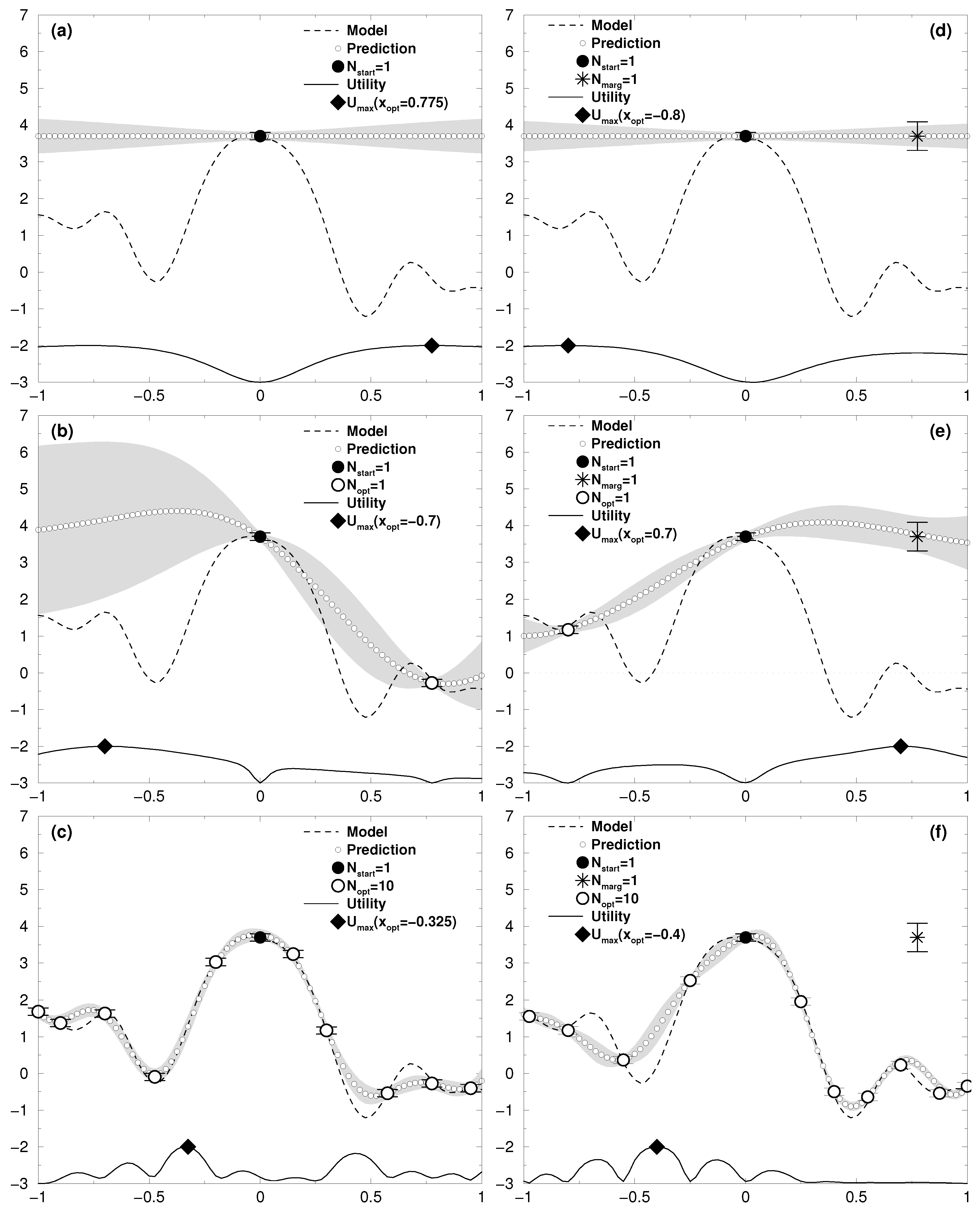
This is plotted in
Figure 1a with
. The
y-value is taken from the sinusoidal model shown (a cos-function with decreasing amplitude), however subjected to whitening, which results in this simple case of one point to the assignment of a zero value. The back-transformation to the scale of the input target value leads to the horizontal line titled “Prediction” (marked by small white circles). As can be seen from Equation (
24), the variance increases with the distance from the data point. The utility according to Equation (
15) was scaled and normalized to fit within the range
of each graph. It produces the result of
for the next best point to measure at. Without marginalization, this would be the input datum returning the results of
Figure 1b for our simple one-dimensional model. After ten iterations, the prediction is—within the gray uncertainty region—almost pinned down to the model generating function (see
Figure 1c).
To run the whole process on a second processor, one would take the first optimal point at
for the marginalization step; i.e., its target value
does not enter the data base. The prediction can also be done analytically to give
with variance
As can be seen in
Figure 1d, the marginalized target point does not affect the prediction much (both
and
are zero after whitening, and yield a zero line according to Equation (
25)). Moreover, the standard deviation of the marginalized point,
, is nearly four times higher than the inputted measurement uncertainty of
, which emphasizes the fact that the marginalized point is of less importance. The utility in
Figure 1d gives rise to the next best point for a measurement at
, but after obtaining the target value, the next utility in
Figure 1e already has its maximum at
, close to the position of the marginalized point
. Together with further points obtained by the optimization procedure, this eventually concludes to a close similarity of the predicted curve with the model (see
Figure 1f). The marginalized point is of no importance, as should be the case.
7. Convergence Study
In this final section, we investigate the convergence behaviour of the results produced by the employed Gaussian process method as a function of an increasing data pool. The quantity to be studied is the total difference between the target values
at all test input vectors
in the region of interest
and the model outcome for these points
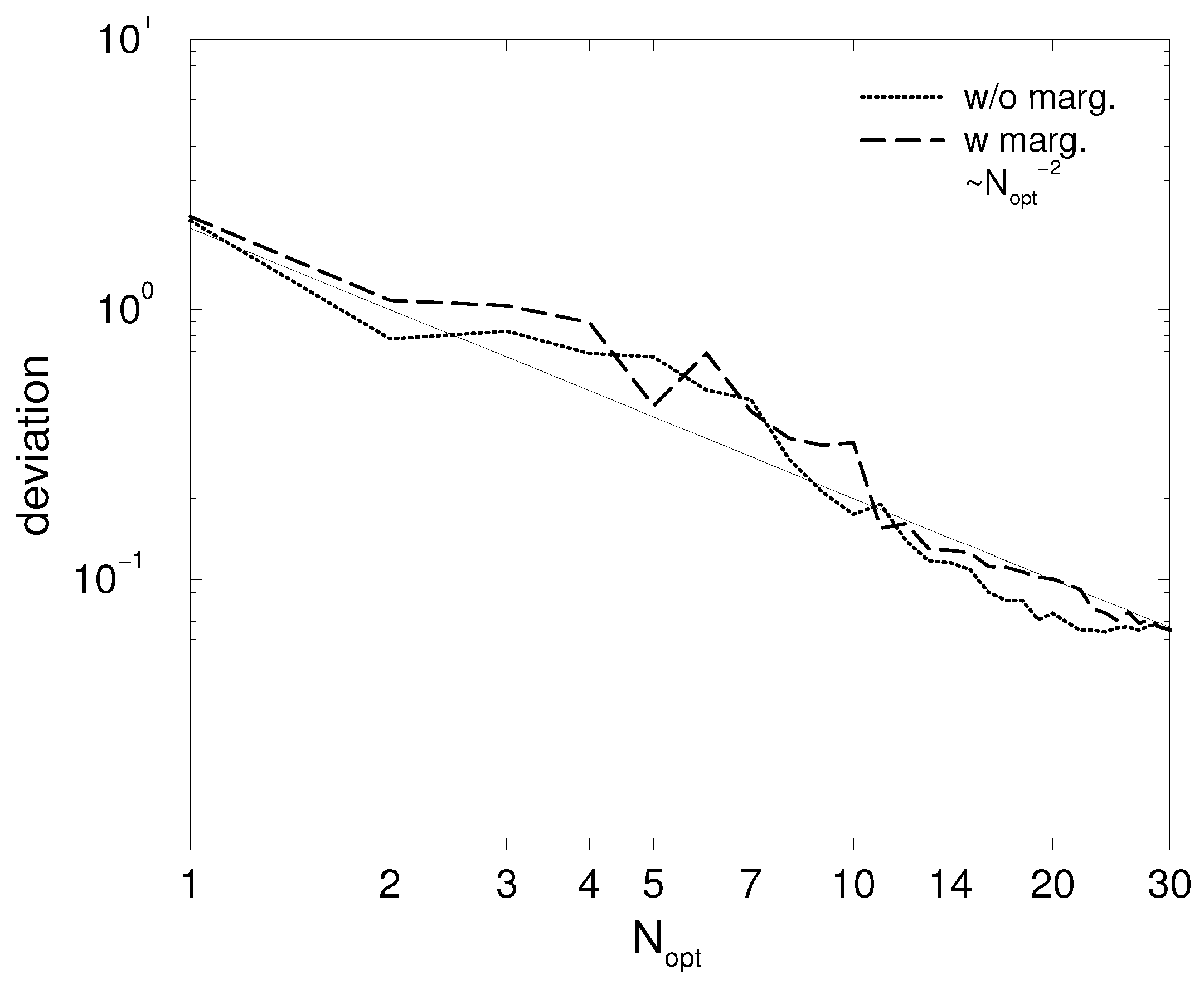
To begin with, we show that the marginalization procedure does not affect the result based on the increasing input data pool. This is supported by
Figure 2, depicting the deviation of the prediction from the model as a function of the number of optimized points in the input data. Both batch runs—with and without marginalization—show the same quadratic descent.
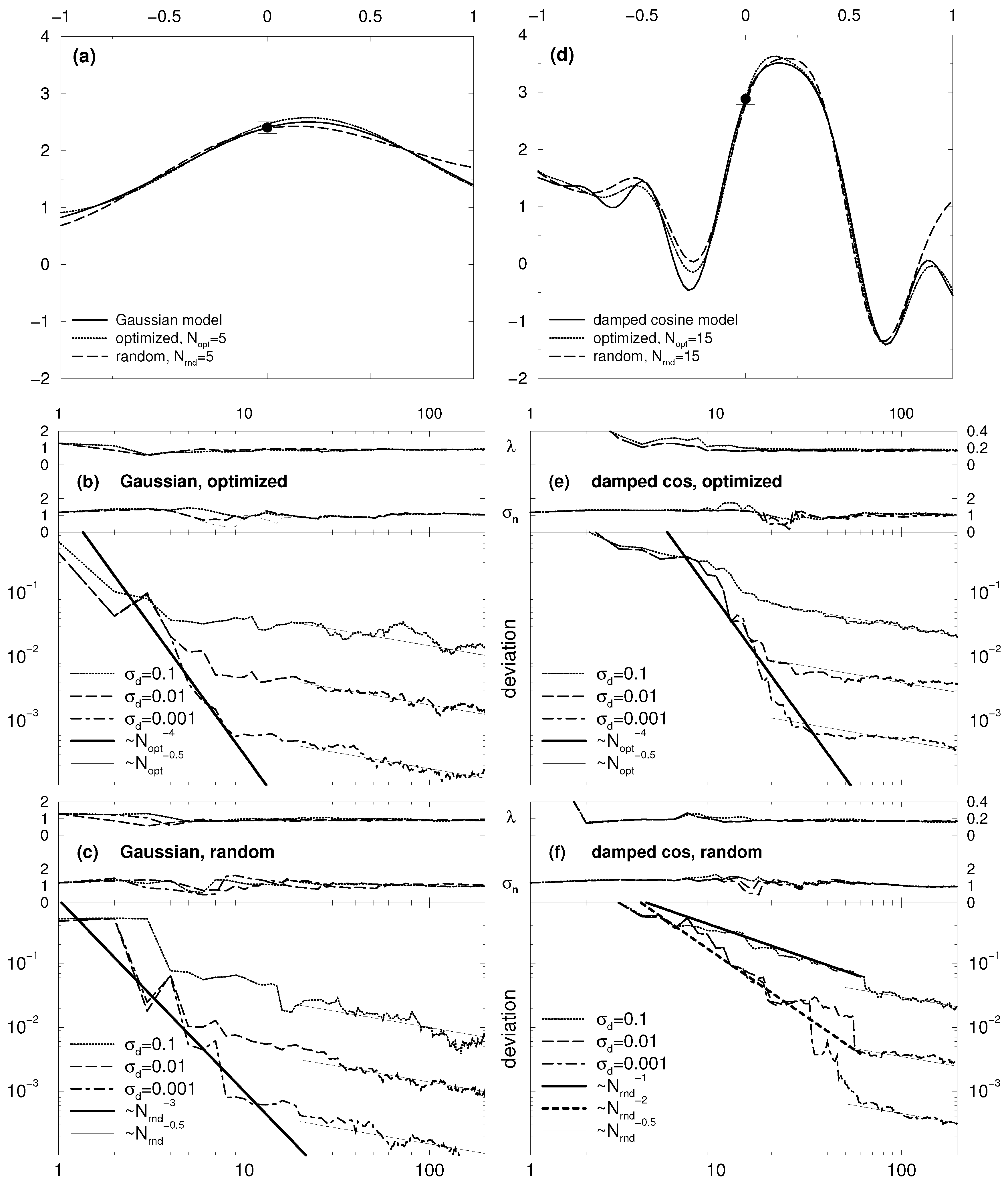
To demonstrate the advantage of the optimized approach over randomly chosen parameter settings, we run two test cases in one and two dimensions (see
Figure 3 and
Figure 4) with different choices of the data uncertainties ranging from 10% over 1% to 0.1% of the total amplitude. Test case one consists of a simple Gaussian with a broad structure, test case two of a damped cosine function sitting on an inclined plane. To avoid artefacts originating from symmetry, the model function was shifted by a value of 0.2 from the center of the ROI. Of interest is the reduction of the variance with the number of acquired data points.
Let us first examine the one-dimensional case shown in
Figure 3. The top row shows the two model functions (thin line), and the result of the Gaussian process method obtained after (a)
= 5 and (d)
= 15 data points were added to the data pool either as the result of the optimization procedure stated in
Section 4 (thick line) or just by randomly chosen parameter settings (dashed line). The result from the optimized approach already covers all features of the respective model function, and is in good agreement with it. The random approach apparently did not choose an input vector close to one in
Figure 3d, and misses the damped progress to the right.
The four
Figure 3b,c,e,f show the convergence behaviour of the deviation Equation (
27). Since the hyper-parameters
λ,
, and
determine the outcome of the Gaussian process method (see
Section 3) and vary a lot in the starting phase of the data acquisition, one has to wait until they have settled. They are plotted in the top of each graph. We restrain from showing
, because it hardly varies for the test cases used. One finds that the hyper-parameters stabilize at about 30 data values added for the damped cosine model, and about 20 for the broad Gaussian. From thereon, the decay of the deviation with the increasing data pool clearly shows square root behavior, while up to this settlement, higher power laws are in charge. The actual values of these higher powers for the decay seem to be somewhat arbitrary, but they are still substantial over all test cases to claim that the optimized approach for finding the best next parameter settings is much more fruitful than to set it up randomly.
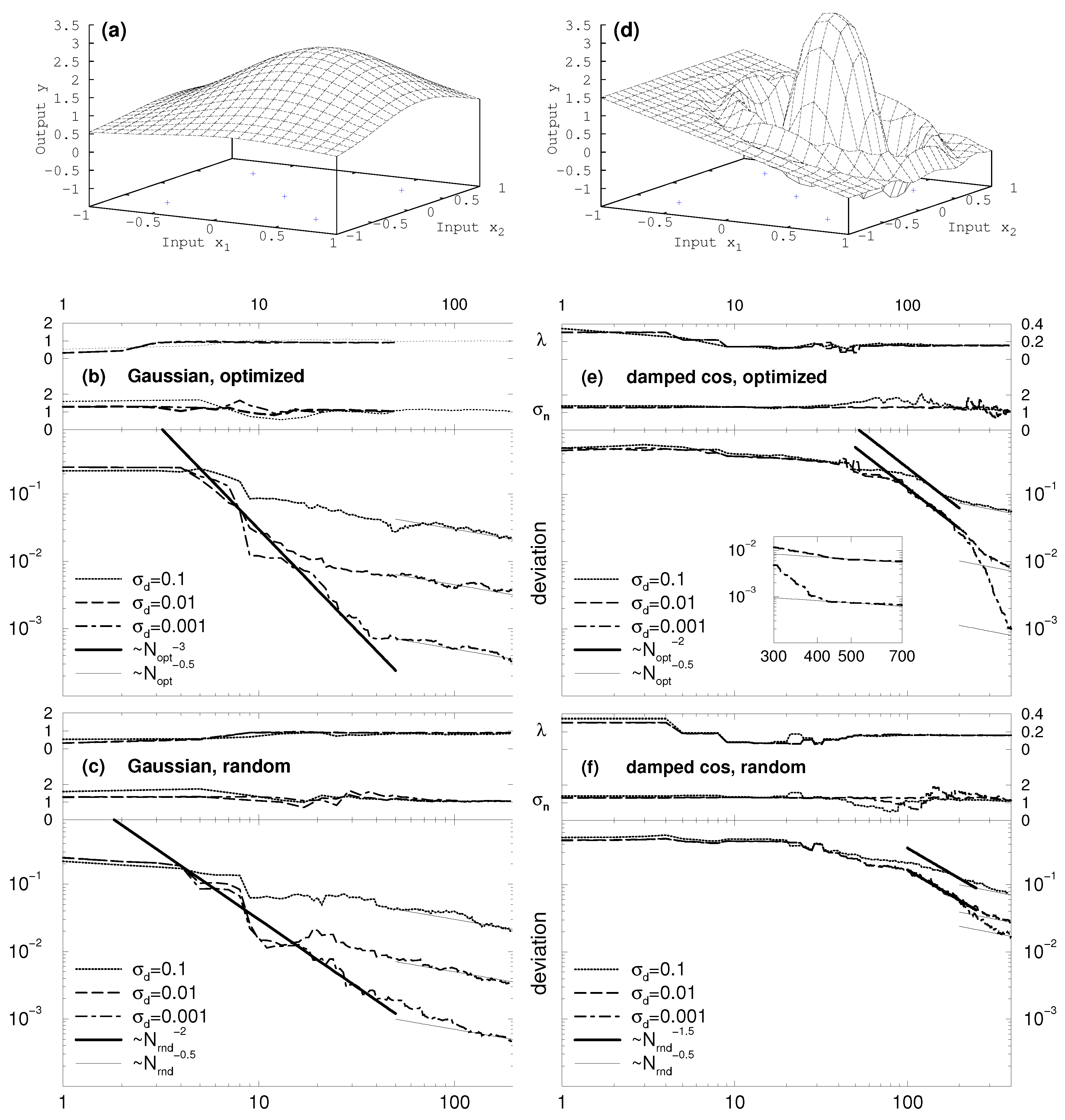
The two-dimensional test cases in
Figure 4 confirm the findings above. Since the small “waves” surrounding the large hump at the center of the damped cosine (
Figure 4d) are much harder to resolve in two dimensions than is the case for the broad structure of the Gaussian (
Figure 4a), the settlement of the hyper-parameters is shifted to higher numbers of acquired data. Again, the optimized approach surpasses the random choice.


