Complexity Analysis of Neonatal EEG Using Multiscale Entropy: Applications in Brain Maturation and Sleep Stage Classification

Abstract

Automated analysis of the electroencephalographic (EEG) data for the brain monitoring of preterm infants has gained attention in the last decades. In this study, we analyze the complexity of neonatal EEG, quantified using multiscale entropy. The aim of the current work is to investigate how EEG complexity evolves during electrocortical maturation and whether complexity features can be used to classify sleep stages. First , we developed a regression model that estimates the postmenstrual age (PMA) using a combination of complexity features. Then, these features are used to build a sleep stage classifier. The analysis is performed on a database consisting of 97 EEG recordings from 26 prematurely born infants, recorded between 27 and 42 weeks PMA. The results of the regression analysis revealed a significant positive correlation between the EEG complexity and the infant’s age. Moreover, the PMA of the neonate could be estimated with a root mean squared error of 1.88 weeks. The sleep stage classifier was able to discriminate quiet sleep from nonquiet sleep with an area under the curve (AUC) of 90%. These results suggest that the complexity of the brain dynamics is a highly useful index for brain maturation quantification and neonatal sleep stage classification.

1. Introduction

According to the World Health Organization (WHO), approximately 15 million babies are born prematurely every year, and the number of births before 37 completed weeks of gestation is still rising [1]. Due to the advancements in the Neonatal Intensive Care Unit (NICU), the survival rates of these infants have increased over the course of severaldecades. However, these babies are more susceptible to brain damage and are prone to neurological impairment. As a result, focus has shifted towards close monitoring of the brain development during the first critical weeks of life [2]. Electroencephalography (EEG) is a valuable noninvasive method for the continuous bedside monitoring of the cerebral function of these vulnerable babies in the NICU. Assessment of the brain maturation by automatic analysis of the neonatal EEG can assist clinicians in starting timely treatment, monitoring the evolution of the baby, and predicting the neurodevelopmental outcome. As a result, a great deal of literature has focused on the extraction of features from the EEG that reflect electrocortical maturation of the neonate (e.g., continuity features [3,4], spectral features [5,6], and connectivity features [7,8]). Besides, the sleep state organization undergoes fast development during their stay in the NICU and provides information about their functional brain maturation. Hence, several algorithms have been developed for automatic sleep stage classification in neonates [9,10]. More recently, attention has focused on nonlinear dynamical analysis of neonatal EEG as well. Few studies have carried out a dimensional analysis of the neonatal EEG during sleep at increasing age [11,12]. They investigated the correlation dimension of a single EEG channel and revealed a positive correlation between the dimensional complexity and the neonate’s age. Furthermore, they observed a significant difference in EEG complexity between the preterm and fullterm population. According to Janjarasjitt et al. [13], the dimensional complexity tends to be higher during active sleep than during quiet sleep. In addition, the sample entropy of the neonatal EEG has been explored by Zhang et al. [14]. They reported an increase of sample entropy up to term age, and found that the sample entropy is higher during active sleep compared to quiet sleep.

In this paper, multiscale entropy will be employed to quantify the complexity of the EEG time series. This method calculates the sample entropy over multiple time scales, exploiting the fact that complex systems are characterized by dynamics at multiple scales. Multiscale entropy has been successfully applied to a wide range of biological signals, such as heart rate variability [15], EEG [16], and electromyography (EMG) [17]. During aging or disease, a reduction of the complexity of the physiologic system is generally observed due the reduced capacity of the system to adapt to stress [18]. The underlying idea for this study is that—in contrast with the loss of the complexity during aging—the rapid changes in the developing brain will result in more complex brain dynamics. We expect that this increase of complexity of the brain dynamics will be reflected in the EEG.

The purpose of this paper is to investigate the EEG complexity measured by multiscale entropy for brain maturation quantification as well as for sleep stage discrimination. To examine the relationship between the complexity measured by multiscale entropy and the postmenstrual age, a correlation and regression analysis have been performed. Besides, in order to identify how the nonlinear brain dynamics relate to the sleep state, a sleep stage classifier based on complexity features has been developed. The performance of these two methods has been tested on a large database of preterm patients to prove that the extracted complexity features can serve as a brain maturation index.

The paper has been organised as follows. First, an overview of the database and the preprocessing of the EEG is given. Secondly, the procedure to compute multiscale entropy is presented. In the following section, the linear regression and classification model will be thoroughly explained. Finally, the findings of this research will be presented and discussed.

2. Materials and Methods

2.1. Database

The dataset used in this study consists of 97 multichannel EEG recordings from 26 preterm neonates with a postmenstrual age (PMA) ranging from 27 weeks to 42 weeks (33.96 ± 3.33 weeks). The neonates included in this study were born prematurely before 32 weeks of gestation (28.74 ± 2.33 weeks). On average, the first EEG recording of each patient was measured 2 weeks after birth (2 days–5 weeks plus 3 days), and serial recordings were performed with at least two recordings per subject. All babies recruited for this study had a normal neurodevelopmental outcome score at 9 and 24 months corrected age.

The EEG signals were recorded between 2012 and 2014 at the Neonatal Intensive Care Unit of the University Hospitals Leuven, Belgium. Informed parental consent was obtained for each recruited patient and the study was approved by the Ethics Committee of the University Hospitals of Leuven. Nine channels of monopolar EEG recording (namely Fp1, Fp2, C3, C4, T3, T4, O1, O2, and reference electrode Cz, recorded using the modified 10–20 EEG recording system) were used. However, the reference channel Cz was disregarded during the analysis. The duration of the EEG recordings ranged from 2 h to 25 h 57 min, with an average recording length of 6 h 57 min. Two independent expert clinicians carried out annotation of quiet sleep segments based on visual analysis of video EEG. Other vigilance states, such as active sleep and awake, are considered nonquiet sleep. In some recordings (mainly in the long EEG measurements from 36 weeks PMA on), the quiet sleep (QS) labelling was stopped before the end of the recording. As a result, the average length of the labelled EEG recordings is 5 h 4 min (1 h 33 min–10 h 9 min). The total quiet sleep duration in the labelled dataset used for the regression analysis is 121 h 41 min. All EEG time series were recorded at a sampling rate of 250 Hz. Neither preselection of data segments, nor artefact rejection has been applied.

The first preprocessing step consisted of resampling all time series to 125 Hz. Next, the EEG signals were bandpass filtered between 1 and 20 Hz, in order to avoid distortion by artefacts while retaining most of the neural activity. The filter was applied twice, once forwards and once reversed, resulting in a zero phase filtering.

2.2. Multiscale Entropy

A well-known method for assessing the complexity of physiological signals is multiscale entropy. Multiscale entropy, developed by Costa et al. [19], quantifies the degree of irregularity of the time series across multiple scales. In contrast with the traditional single-scale entropy measures, multiscale entropy can account for structures with long-range correlations on multiple time scales present in complex systems, and will not assign a high complexity to completely random signals which are not truly complex [19,20].

The procedure to compute the multiscale entropy of a signal consists of two steps. The signal is first coarse-grained according to the scale factor $\tau$. The time series {$x_1$,$x_2$,…,$x_i$,…$x_N$} is segmented into nonoverlapping windows of length $\tau$ and the mean of the data points in each of these windows is computed. Thus, each element of the coarse-grained time series is computed as:

$$y_j^{\tau }=\frac{1}{\tau }\sum _{i=(j-1)\tau +1}^{j\tau }{x}_i,1\le j\le \frac{N}{\tau }$$

resulting in a new time series $y^{\tau }=\{y_j^{\tau },j=1,\dots ,\frac{N}{\tau }\}$. This coarse graining procedure corresponds to applying a moving average filter $\left(y_j^{\tau }=\frac{1}{\tau }{\displaystyle \sum _{k=0}^{\tau -1}}x(j-k),1\le j\le N\right)$ followed by downsampling with a factor $\tau$ [21,22]. The length of the coarse-grained time series is equal to the length of the original signal divided by the scale factor $\tau$. At scale 1, the original time series will be obtained. The next step is to calculate the sample entropy for each coarse-grained time series. Sample entropy is a measure of irregularity or unpredictability of the signal. It is calculated as the negative natural logarithm of the conditional probability that two sequences of m consecutive points similar within a tolerance r will also be matching if an extra point is added to the sequence [23].

The tolerance is typically set as a percentage of the standard deviation of the original time series. This normalization prevents the result from beingaffected by the variance of the signal [19,23]. In the present paper, the embedding dimension m was chosen equal to 2 and tolerance was set as 0.2× standard deviation [14,24]. Eventually, the output of the multiscale entropy analysis is a curve of sample entropy in function of scale [19].

Prior to computing the multiscale entropy of the neonatal EEG time series, the signals were segmented into epochs of length N. There are multiple factors to take into account when optimizing the window length. To acquire a reliable entropy estimate, the number of data points should be large enough [19]. If the window length is too short, it is possible that no template matches will be found, hence the entropy will be undefined. An important consideration in the choice of the window length N is that the length of the coarse-grained sequence is reduced progressively with increasing scale. In this study, the largest analyzed scale $\tau$ is equal to 20, thus the shortest sequence will have length $\frac{N}{20}$. 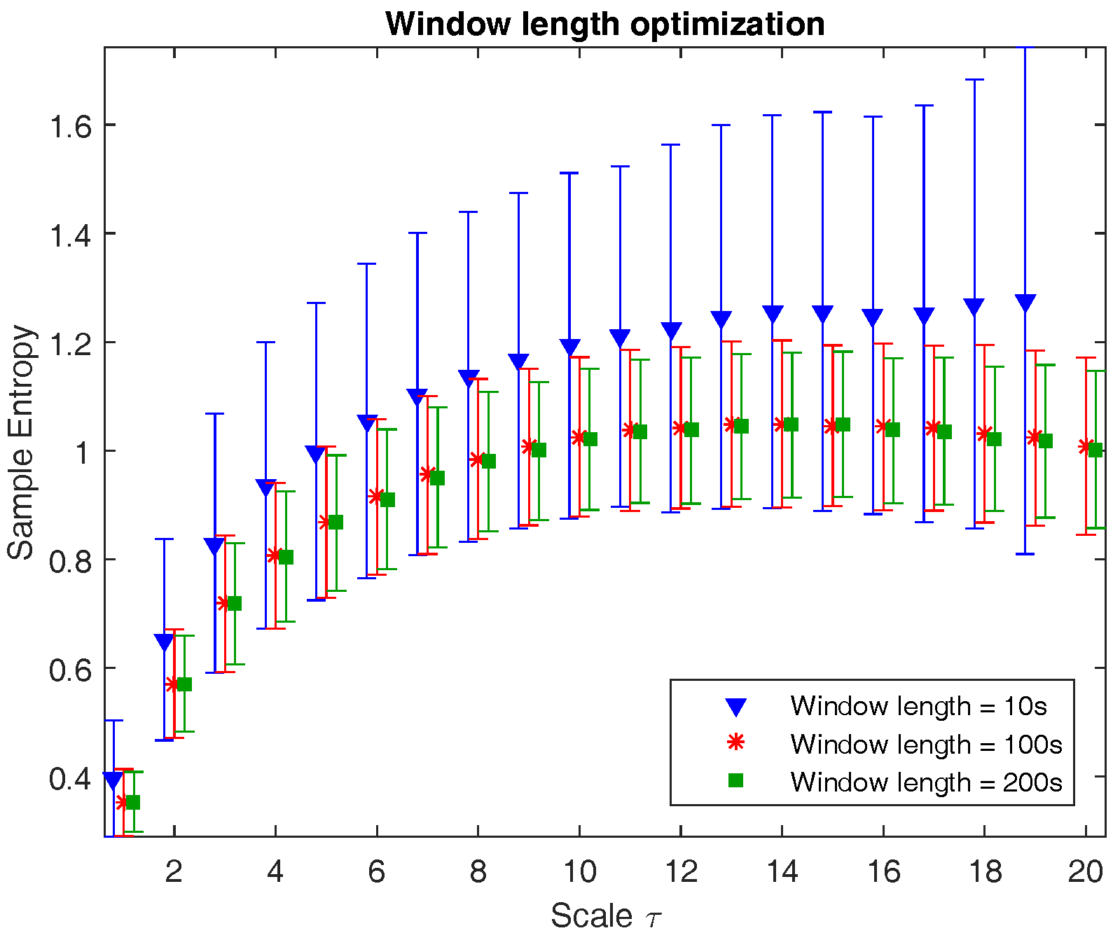Figure 1 illustrates the multiscale entropy of channel C3 of a neonatal EEG recording during quiet sleep evaluated at three different window lengths: 10 s (1250 samples), 100 s (12,500 samples), and 200 s (18,750 samples). The graph shows that from a certain window length on, the mean is no longer affected, while the standard deviation slightly reduces with longer epochs. However, the computational time is inversely proportional to the window length. As a result, the choice of window length is a trade-off between accuracy, robustness, and computational time. Since the reduction in standard deviation in 200 s versus 100 s is negligible and the computational time is reasonable, the window length is chosen to be equal to 100 s.

2.3. Feature Extraction

After quantifying the multiscale entropy of each EEG channel, four features were extracted from the multiscale entropy curve: (1) the area under the multiscale curve (this will be referred to as the complexity index); (2) the average slope of the multiscale entropy curve in the small scales (scale 1–5); (3) the average slope of the curve in the large scales (scale 6–20); and (4) the maximum value of the multiscale entropy curve. Thus, in total, a set of 32 (8 channels × 4) features are extracted. A correlation analysis and linear regression will be performed in order to investigate the relationship between the complexity features and the patient’s age during quiet sleep. Moreover, a classifier to discriminate quiet sleep from nonquiet sleep using these features will be developed. A more elaborate description of the regression and classification model are given in the next sections.

2.4. Correlation and Linear Regression Analysis

To prepare the feature matrix for the correlation and linear regression analysis, all data points during quiet sleep within a recording were averaged, resulting in one data point for each recording (97 in total). The Pearson correlation coefficient $\rho$ between each of the complexity features and the response variable was then computed using the complete dataset. Moreover, the number of times that this correlation was significant (p < 0.05) was calculated.

To increase the robustness and reliability of the results, the regression analysis was repeated 100 times, and in each iteration the dataset was randomly split into a training and test set with a 70–30 ratio. The training set was used to build the model, while the prediction error of the model was assessed on the independent test set. The median and interquartile range of the performance measures are reported. For each complexity feature, a linear regression model explaining the relationship between the feature and the PMA was estimated on the training set. The coefficient of determination, $R^2$, was computed for the test set as: $R_{test}^2=1-\frac{\Sigma {(y_{test}-{\hat{y}}_{test})}^2}{\Sigma {(y_{test}-{\overline{y}}_{test})}^2}$, where $y_{test}$ denotes the observed response variable, ${\overline{y}}_{test}$ is its mean, and ${\hat{y}}_{test}$ is the corresponding predicted value [25]. Finally, the PMA estimation is evaluated on the test set using the square root of the mean squared error ($\sqrt{MSE}$).

In the second step, several complexity features were combined in a multiple regression. First, features that did not have a significant correlation with the response variable were removed. Afterwards, selection of the most relevant features was carried out using the least absolute shrinkage and selection operator (LASSO) algorithm. This method forces regression coefficients to zero and tends to avoid collinear predictors [26]. The LASSO algorithm was performed 100 times, and the features that were selected more than 80 times were withheld to build the multiple regression model. The $R^2$ is again computed for the test set. At last, the predictive power of the model is quantified by computing the root mean squared error of the test set.

2.5. Sleep Stage Classification

To investigate how powerful the complexity features are in identifying neonatal sleep stages, a sleep stage classifier was developed using LS-SVMlab [27,28]. The complete feature matrix X $\in {\mathrm{I}\mathrm{R}}^{N\times d}$ consists of N = 17,600 datapoints ($N_{QS}$ = 4356, $N_{NQS}$ = 13,244) and d = 32 features. To cope with the large number of datapoints, a fixed-size least squares support vector machine (LS-SVM) was adopted. This method selects a (small) fixed number of training datapoints M (M ≪ N) representing the underlying distribution of the dataset through maximization of the quadratic Renyi entropy [29]. A Radial Basis Function (RBF) kernel was used during this active selection of the support vectors, and its bandwidth parameter was computed according to the rule of thumb: ${\sigma }^2$ = factor × d × mean[var(X)], where d is equal to the number of features, and var(X) = [var($x_1$) var($x_2$) ... var($x_d$)] with $x_i\in {\mathrm{I}\mathrm{R}}^N$ [30]. The factor was tuned experimentally and set equal to 0.1. The number of support vectors M that are selected in an iterative way was set equal to 1500.

As we expect that the maturational effect will also play a role during sleep stage classification, the observations were divided into three groups according to their PMA: recordings before 31 weeks ($N_{<31}$ = 2395), in the range from 31 to 37 weeks ($N_{31-37}$ = 10,901), and EEGs recorded beyond 37 weeks PMA ($N_{>37}$ = 4304) [31]. To assure that not all training datapoints were drawn from 1 sleep state, the number of training datapoints selected from a specific sleep state was proportional to its representation in the complete dataset. Similarly, the ratio of the number of observations for a specific age group was preserved.

The hyperparameters of the LS-SVM model with Gaussian RBF kernel were then tuned using 10-fold cross-validation, resulting in a regularization parameter $\gamma$ = 52.02 and a squared bandwidth ${\sigma }^2$ = 283.88. After training the LS-SVM classifier, the classification performance was tested on all remaining samples. As the complexity of the EEG is expected to evolve throughout age as well, we are interested in both the overall classification performance and in the classification power for each of the age groups separately. The receiver operating characteristic (ROC) curves will be constructed for the four test sets and the performance will be measured as the area under the curve (AUC).

2.6. Topological Analysis

In addition to the evolution of EEG complexity with age and sleep stage, topological differences are of great interest as well. Since the complexity features were computed for each of the EEG channels, it is possible to investigate how the complexity changes are dependent on the brain region. For this analysis we focused on the complexity index (area under the multiscale entropy curve) and we divided the recordings into four age groups: below 31 weeks, from 31 to 34 weeks, from 34 to 37 weeks, and above 37 weeks. The spatial map was then computed by taking the group average of the complexity index during a specific sleep stage for a specific age range. In addition, we explored whether there is a dominance of 1 of the 2 brain hemispheres.

3. Results

In this section, the results of the neonatal EEG complexity analysis will be presented. The first section focuses on the results of the linear regression analysis and will indicate how well a combination of complexity features can predict the PMA of a neonate. The second section provides the results of the sleep stage classification based on these features. At last, the observed topological changes of the complexity index will be briefly summarised.

3.1. Linear Regression Analysis

After performing a correlation analysis between each feature and the response variable, the significance of the correlation was checked. The eight features representing the average slope in the large scales were removed, since for most channels these features did not have a significant correlation with age. All the remaining features had a significant positive correlation with PMA.

The LASSO algorithm selected a subset of 16 features; all of these were chosen at least 96 out of 100 times (see the last column of

Table 1. The top of the table provides the results of the correlation and regression analysis for each feature that has been selected by the least absolute shrinkage and selection operator (LASSO) algorithm separately. The bottom of the table presents the performance of the multiple regression combining all 16 features. The correlation coefficient $\rho$ for the complete dataset, and the median and interquartile range of the $R^2$ and root mean squared error for the test set are set out. The last column indicates how many times each feature was selected by LASSO.

Feature(s)		$\mathbf{\rho }$	${\mathbf{R}}_{\mathbf{test}}^{\mathbf{2}}$	$\sqrt{\mathit{M}\mathit{S}\mathit{E}}$ (wks)	# Selected LASSO
Complexity Index	C3	0.76	0.54 (0.19)	2.17 (0.52)	99
	T3	0.81	0.66 (0.14)	1.93 (0.42)	100
Average slope in small scales	Fp1	0.76	0.56 (0.19)	2.17 (0.49)	99
	Fp2	0.75	0.53 (0.19)	2.19 (0.39)	99
	C3	0.78	0.55 (0.19)	2.16 (0.45)	99
	C4	0.80	0.64 (0.14)	1.96 (0.40)	100
	T4	0.80	0.61 (0.15)	2.01 (0.56)	100
	O1	0.78	0.61 (0.17)	2.03 (0.38)	99
	O2	0.77	0.56 (0.16)	2.15 (0.36)	100
Maximum of multiscale entropy curve	Fp1	0.77	0.59 (0.15)	2.12 (0.30)	99
	Fp2	0.76	0.52 (0.19)	2.25 (0.52)	99
	C4	0.79	0.60 (0.18)	2.03 (0.39)	96
	T3	0.80	0.61 (0.15)	1.98 (0.49)	99
	T4	0.79	0.61 (0.17)	2.00 (0.44)	100
	O1	0.75	0.55 (0.18)	2.19 (0.38)	99
	O2	0.74	0.52 (0.11)	2.31 (0.29)	99
Combination of 16 selected features			0.69 (0.13)	1.88 (0.36)

). The top part of Table 1 shows the results of the correlation and regression analysis for each of the chosen features separately. Each of the single predictors could estimate the age of the neonate with a $\sqrt{MSE}$ in the range of 1.93–2.31 weeks.

The performance of the multiple regression model, where all 16 features selected by LASSO are combined, is presented in the bottom of Table 1. Using this model, the age of the neonate could be estimated with a root mean squared error of 1.88 weeks and a coefficient of determination of 0.69.

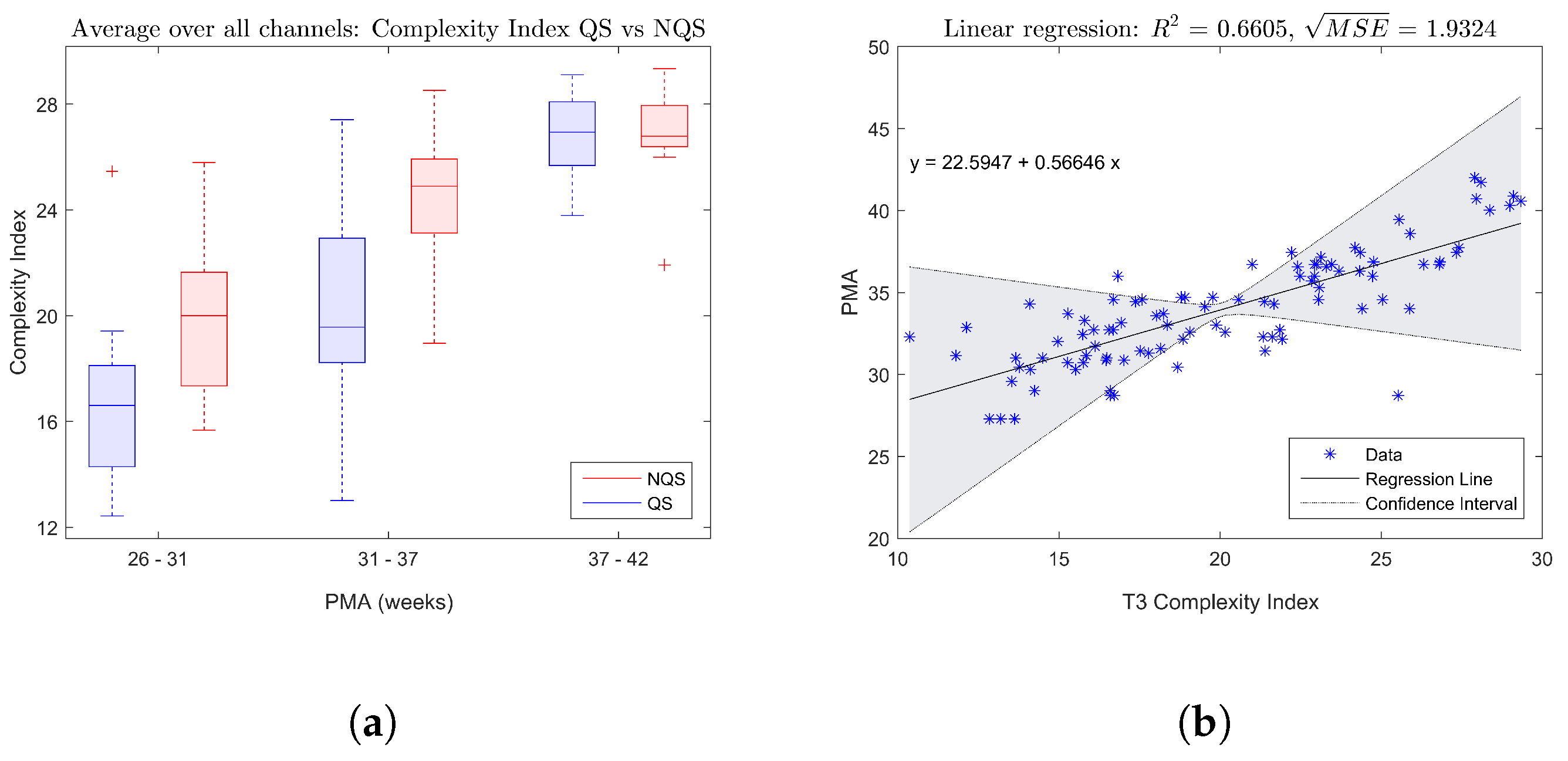
The boxplot in Figure 2a shows the trend of the complexity index averaged over all EEG channels with increasing age, while Figure 2b gives an example of a fitted linear regression model for the complexity index of electrode T3. Both figures confirm that there is a significant increase of the complexity of the brain dynamics during maturation.

3.2. Sleep Stage Classification

This part of the analysis aimed to investigate how the complexity of the EEG changes dependent on the vigilance state. First of all, the boxplot in Figure 2a indicates that on average the complexity index tends to be higher during nonquiet sleep compared to quiet sleep.

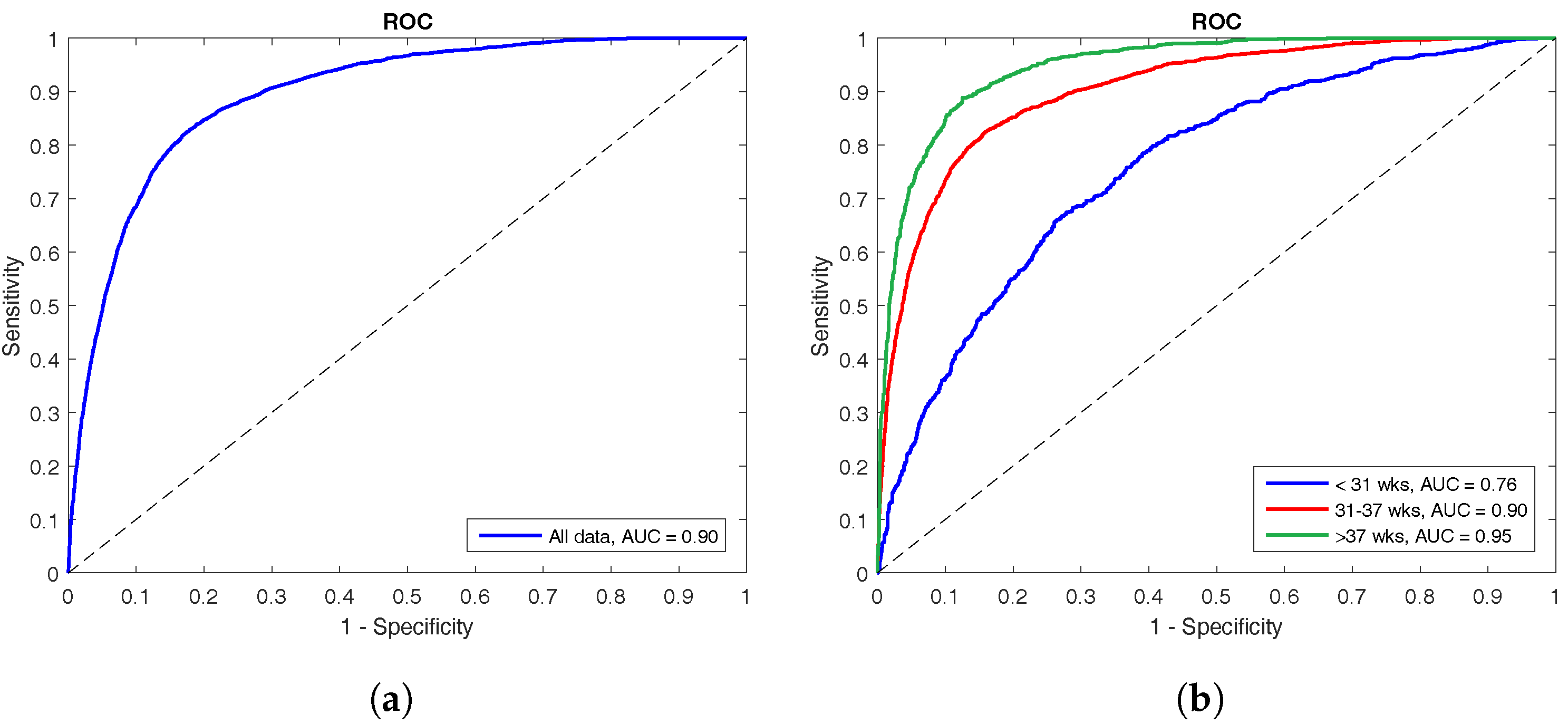
The performance of the LS-SVM classifier is shown by means of ROC curves in Figure 3. The left panel shows the ROC curve for the complete test set with an AUC of 90%, whereas the right panel illustrates how the classifier performs on the different age groups. The oldest group has the best performance with an AUC of 95%, the middle group has an AUC of 90%, and the classifier performed worst at the youngest age with an AUC of only 76%.

3.3. Topological Analysis

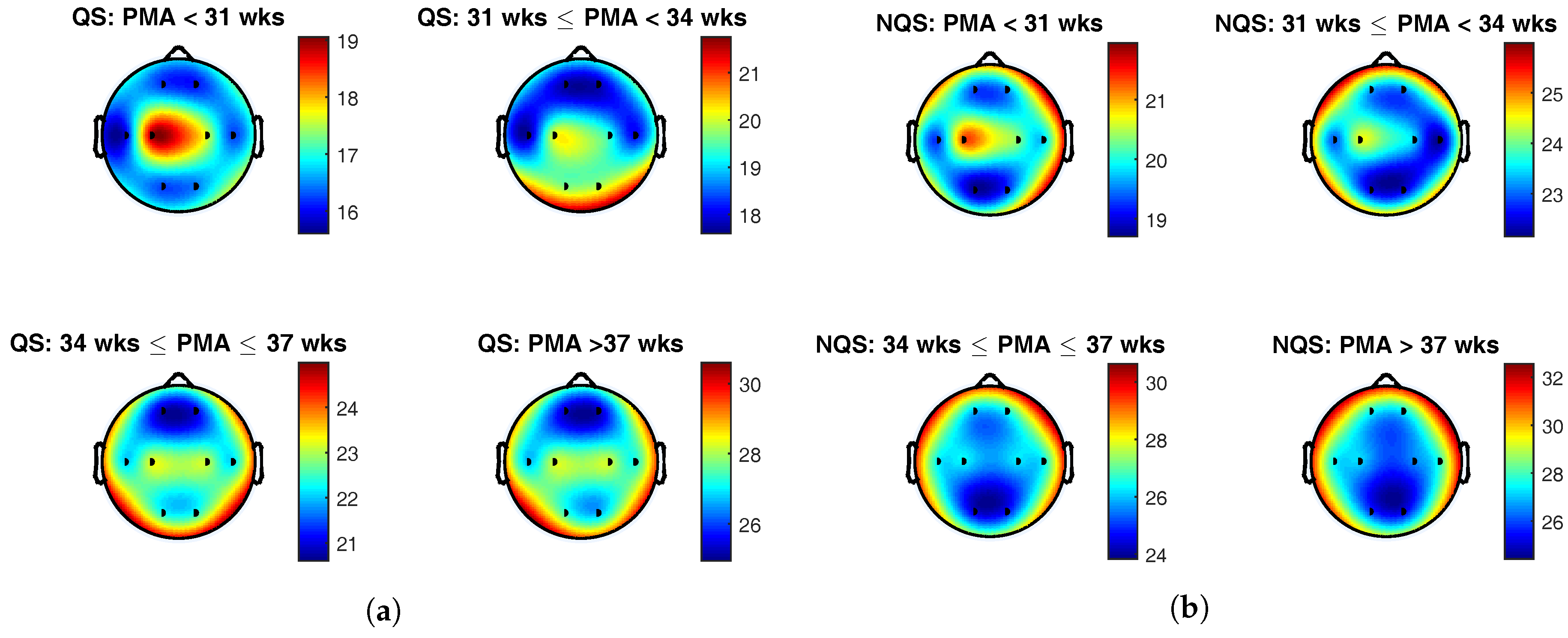
The topoplots of the group average of the complexity index during quiet sleep and nonquiet sleep are presented in Figure 4a,b, respectively. The color indicates the value of the complexity index at the different brain areas, and the black dots represent the position of the eight EEG electrodes.

To begin with, the colorbars show a rise of the complexity index with postmenstrual age within each sleep state. On top of that, comparison of the colorbars between the vigilance states for the same age group reveals that complexity index was generally higher during nonquiet sleep than during quiet sleep. These findings confirm the results of the correlation analysis described above and is in line with the trends that can be seen in the boxplots in Figure 2a.

From Figure 4a, it can be seen that the central derivation was dominant below 31 weeks PMA during quiet sleep. In the second age group, from 31 to 34 weeks PMA, the EEG complexity exhibited the highest value in the central and occipital regions. From 34 weeks PMA onwards, the temporal electrodes gained importance as well. Beyond 34 weeks PMA, the spatial maps remained static, with highest EEG complexity in the central, temporal, and occipital regions.

During nonquiet sleep, the topological changes in brain complexity were less pronounced. As during quiet sleep, central complexity predominated at the youngest age. Between 31 and 34 weeks PMA, a spread towards the frontocentral region can be observed. In the oldest age groups, the frontotemporal areas exhibited the highest complexity index.

However, conclusions drawn from these topoplots should be interpreted with caution, as only the group average was investigated and the variability among the recordings was disregarded.

4. Discussion

This study was set out with the aim of assessing the neural complexity of multichannel EEG recordings in preterm infants. The first part of the analysis demonstrated that there was a significant positive correlation between the EEG complexity and the PMA. Moreover, we have predicted the age of the patient using a regression model based on EEG complexity features. In the second part of the analysis, these complexity features were employed to build a neonatal sleep stage classifier. The high performance of this classifier indicates that the complexity of brain dynamics exhibit fundamental differences between vigilance states in preterm infants. To conclude, the spatiotemporal plots of the complexity suggest that the central area is most complex below 31 weeks in both sleep states. During quiet sleep, the predominance of the central area shifts towards the occipital and temporal regions with increasing age.

The maturational trend observed in the complexity features confirms the hypothesis and is in line with the results of prior studies [11,12]. This increase in EEG complexity can be attributed to changes in the dynamics of the underlying neural networks during cortical maturation [13]. In this paper a regression model, relying solely on complexity features, is used to predict the patient’s PMA. The best estimate of the PMA has a $\sqrt{MSE}$ of 1.88 weeks, which is comparable to the results reported in [6,32].

In accordance with literature, we found that the neural complexity is dependent on the sleep stage [13,14]. By developing a classification model that is able to identify neonatal sleep stages, the present study contributes additional evidence suggesting that brain dynamics are different in quiet sleep compared to nonquiet sleep. It is interesting to note that the performance of the proposed sleep stage classifier depends on the PMA. A possible explanation for this might be the maturational effect. Even though sleep state organization starts at 27 weeks, sleep–wake cycles can only be differentiated at around 31 weeks PMA [33]. Therefore, sleep stage discrimination below 31 weeks is challenging both for clinicians and for the algorithm. Another factor that may explain the worst performance for recordings before 31 weeks PMA is the imbalance of the age groups. With only 14% of the training data coming from recordings of the youngest age group, this group is underrepresented in the training set. As a consequence, the classifier might be biased towards other, more represented, age groups. In contrast with the approach taken here, it is also possible to train a separate classifier for the different age groups. These age-specific models will probably outperform the presented classifier. However, since the model is tailored to a specific PMA range, it will be less useful in clinical practice.

By computing the complexity for all EEG channels, spatiotemporal information can be extracted. This topological analysis can shed more light on the electrophysiological aspects of the study. One of the hallmarks of preterm EEG are delta brushes. At first these complexes tend to appear in the central brain regions; from around 31 weeks onwards they become more predominant in the temporal-occipital regions [34]. This pattern, with the dominant area moving from the central towards temporal-occipital regions, corresponds to what is observed in the topoplots of the complexity during quiet sleep. The patterns in the spatial maps during nonquiet sleep are more difficult to interpret. The dominance of the central regions at the youngest age corresponds to what has been found during quiet sleep, but we could not find a clinical explanation for the spread towards the frontal and temporal areas with increasing age. This might be due to the fact that nonquiet sleep incorporates both active sleep and being awake. Moreover, artefacts are more likely to occur during nonquiet sleep and might have affected the spatial maps.

The presented research has multiple clinical implications. To begin with, the results of the analysis show that the neonatal EEG complexity is a marker of brain maturation and can assist clinicians in evaluating the neurological function of the infant. Moreover, aberrations in the complexity features can play a major role in identifying neonates at increased risk for neurodevelopmental delay which need close cot-side EEG monitoring. In this way, neuroprotective interventions can be started early after diagnosis and the efficacy of the therapy can be monitored.In addition, we proved that the complexity features can be used to automatically classify neonatal sleep stages. Since the sleep state organization is evolving throughout maturation, sleep–wake cycling can provide information about the neurological well-being of the infant. Besides, sleep stage monitoring is practical in order to promote ideal neonatal sleep and avoid disruption of the infant’s sleep during care routines in the NICU.

In the present study, promising results were obtained using multiscale entropy to analyse the complexity of the neonatal EEG. However, extensions of multiscale entropy or other advanced methods to assess signal complexity can be adopted in future investigations [35,36]. One of the limitations of the current study is that the EEG was only recorded in neonates with normal neurodevelopmental outcome up to 42 weeks PMA. According to the existing literature and the well-known “loss of complexity”, a reduced complexity of the brain dynamics is expected in preterm infants with poor outcome [18,24]. In order to confirm this hypothesis, further research in a cohort with unfavourable prognosis must be carried out. Moreover, to develop a full picture of the EEG complexity, future investigations must establish the behaviour of the EEG complexity beyond 42 weeks PMA. On top of that, an important issue for future research is to reveal how the observed complexity changes are related to structural changes in the underlying brain structure. For this purpose, a simultaneous neuroimaging study would be of great interest. Since the results presented in this paper strengthen the idea that the EEG complexity is highly useful in tracking brain maturation, and linear and nonlinear features can provide complementary information, a natural progression of this work is to combine the presented nonlinear complexity features with previously developed features to quantify neurodevelopment.

5. Conclusions

In this paper, we investigate how the complexity of the EEG can be used to quantify brain maturation and to classify sleep stages in preterm infants. A multiple regression model based on a combination of EEG complexity features derived from the multiscale entropy curves could predict the age of the neonates with a $\sqrt{MSE}$ of 1.88 weeks. Moreover, a classifier relying on these features could identify neonatal sleep stages with an AUC of 90%. These findings indicate that EEG complexity is able to quantify brain maturation and discriminate neonatal sleep stages. In summary, these results show that EEG complexity is a valuable feature in the neuromonitoring of preterm infants.