Article

Solution of Higher Order Nonlinear Time-Fractional Reaction Diffusion Equation

by
Neeraj Kumar Tripathi
1,†,
Subir Das
1,†,
Seng Huat Ong
2,†,
Hossein Jafari
3,4,*,† and
Maysaa Al Qurashi
5,†
1
Department of Mathematical Sciences, Indian Institute of Technology (BHU), Varanasi 221 005, India
2
Institute of Mathematical Sciences, University of Malaya, Kuala Lumpur 50603, Malaysia
3
Department of Mathematical Sciences, University of South Africa, UNISA, Pretoria 0003, South Africa
4
Department of Mathematics, University of Mazandaran, Babolsar 47416, Iran
5
Department of Mathematics, King Saud University, Riyadh 11495, Saudi Arabia
*
Author to whom correspondence should be addressed.
Entropy 2016, 18(9), 329; https://doi.org/10.3390/e18090329
Submission received: 8 July 2016 / Revised: 30 August 2016 / Accepted: 31 August 2016 / Published: 8 September 2016
(This article belongs to the Special Issue Wavelets, Fractals and Information Theory II)

Abstract

:
The approximate analytical solution of fractional order, nonlinear, reaction differential equations, namely the nonlinear diffusion equations, with a given initial condition, is obtained by using the homotopy analysis method. As a demonstration of a good mathematical model, the present article gives graphical presentations of the effect of the reaction terms on the solution profile for various anomalous exponents of particular cases, to predict damping of the field variable. Numerical computations of the convergence control parameter, used to evaluate the convergence of approximate series solution through minimizing error, are also presented graphically for these cases.

1. Introduction

Nonlinear diffusion equations, an important class of parabolic equations, have come from a variety of diffusion phenomena which appear widely in nature. These are suggested as mathematical models of physical problems in many fields, such as filtration, phase transition, electromagnetism, acoustics, electrochemistry, cosmology, biochemistry and dynamics of biological groups. In many cases, the equations possess degeneracy or singularity, which makes the study more involved and challenging. Ultimately, this degeneracy or singularity has enriched the theory of partial differential equations. Science and engineering problems are generally nonlinear, therefore it is important to generate new efficient methods to solve such nonlinear problems. With the help of computerized symbolic computations, many researchers have implemented various methods to establish the solutions to different nonlinear differential equations e.g., the Exp-function method, the Jacobi elliptic function expansion method, the first integral method, the (G’/G)-expansion method, the direct algebraic method, the Cole-Hopf transformation method [1,2,3,4,5,6,7,8] and others. Fractional differential equations are considered as the general form of the differential equations that involved derivatives of any real or complex order. Over the years, fractional calculus has attracted the interest of engineers and scientists immensely.
Fractional differential equations are considered as the general form of differential equations, as they are involved with the derivatives of any real or complex order. In recent years, fractional calculus has attracted the interest of engineers and scientists immensely. The history and the comparative treatment of fractional order have been given by Oldham and Spanier [9], Miller and Ross [10] and Podlubny [11]. The phenomena, which occurs in engineering physics and other branches of science, can be described very successfully. Fractional partial differential equations have comprehensive applications in real world problems compared to integer order ones. Fractional partial differential equations are found to be an effective tool to describe certain physical phenomena, such as diffusion processes and visco-elasticity theories. In this article, we consider a type of time fractional partial differential equation that can be obtained from a standard diffusion equation by replacing the first order time derivative with the Caputo fractional order α , 0 < α < 1 , with higher order nonlinear diffusive and reaction terms. Fractional differential equations have been applied in the modeling of anomalous diffusive and sub-diffusive systems, description of fractional random walk, unification of diffusion. Due to the importance of differential equations of fractional order, many authors are working to find the exact or numerical solutions of the equations. Various methods for obtaining numerical solution have been applied, such as the artificial parameter method, the fractional sub-equation method, the δ -expansion method, the homotopy perturbation method, the generalized differential transform method, the finite difference method, the power series method, and the Exp-function method etc. In 1992, the Chinese mathematician Liao [12] first introduced homotopy to propose an analytic method for the strongly nonlinear problem of the homotopy analysis method (HAM). Thereafter, the HAM has been improved step by step and has been widely applied for solving the nonlinear problems. The advantages of using the HAM as the solution for the nonlinear problems, are that the method is always valid no matter whether there are small physical parameters or not; it provides a simple way to guarantee the convergence of approximation series and it has the flexibility to choose the equation type of linear sub-problems and the base functions of solutions. The main advantage of the HAM is that it always provides a simple way to adjust and control the convergence radius of solution series. Another benefit is that, by studying the HAM in the wide context, we are actually able to obtain a more general iteration method which may exhibit better convergence properties [13,14,15,16,17,18].
The method is a useful analytical approach to get the series solution of fractional order linear and nonlinear partial differential equations (PDEs). This method has certain advantages over some existing numerical methods. Due to discretization used in numerical methods, loss of accuracy during the rounding of errors is possible and also computation requires much time. However, in HAM there is no need for a discretization of variables and it requires less time for computation. Many researchers [19,20,21,22,23,24,25,26,27,28,29,30,31,32,33,34,35,36,37,38,39] have used the method for handling linear and nonlinear problems in fractional order systems.
In this article, an effort has been made to solve a nonlinear fractional order reaction diffusion equation using the HAM. Here, diffusive term is taken as a cubic order polynomial and the reaction term is taken as cubic order. The approximate analytical solution of the equation is found using the powerful technique HAM. The salient feature of the article is the graphical presentation of the probability density function u(x,t) with and without the presence of highly nonlinear reaction term for different Brownian motions and also for the standard motion.
The paper is organized as follows. In Section 2, some necessary definitions of the fractional calculus are provided. In Section 3, the HAM is introduced. In Section 4, we have successfully applied the HAM on time nonlinear fractional order diffusion equation with higher order reaction term. Section 5 consists of the discussion of numerical calculations of the obtained result, followed by a conclusion consisting of the overall work and a future study given in Section 6.

2. Definitions

(a)
A real function f ( x ) , x > 0 is said to be in the space C λ , λ if a real number q ( > λ ) , such that f ( x ) = x q g ( x ) , where g ( x ) C [ 0 , ) . Clearly C λ C μ if μ λ .
(b)
A function f ( x ) , x > 0 is said to be in the space C λ m , m N { 0 } if f ( m ) C λ .
(c)
The (left sided) Riemann–Liouville fractional integral of order δ > 0 of a function f C λ , λ 1 is defined as J δ f ( t ) = 1 Γ ( δ ) 0 t f ( τ ) ( t τ ) 1 δ d τ , δ > 0 , t > 0 where J 0 f ( t ) = f ( t ) .
(d)
The (left sided) Riemann–Liouville fractional derivative of f , f C 1 m , m N { 0 } of order δ > 0 , is defined by D δ f ( t ) = J m δ d m d t m f ( t ) , m 1 < δ m , m N .
(e)
The (left sided) Caputo fractional derivative of f , f C 1 m , m N { 0 } is defined as
D δ f ( t ) = { J m δ f ( m ) ( t ) ,   m 1 < δ < m ,    m N , d m d t m f ( t ) ,    δ = m .

3. Basic Idea of HAM

Perturbation techniques are widely applied to obtain analytic approximations of nonlinear equations. However, perturbation methods are essentially based on small physical parameters known as perturbation quantity, but unfortunately many nonlinear problems have no such kind of small physical parameters at all. In addition, neither perturbation techniques, nor the traditional non-perturbation techniques, can provide a way to guarantee the convergence of approximation series. Therefore, both perturbation techniques and the traditional non-perturbation methods mentioned above are, in essence, valid only for weakly nonlinear problems.
We consider the following differential equation
N [ U ( x , t ) ] = 0   ,
where N is a nonlinear operator, r and t are independent variables, u ( x , t ) is an unknown function. By means of generalizing the traditional HAM, Liao [14] constructed the so-called zero-order deformation equation as
( 1 q ) £ [ U ( x , t ; q ) u 0 ( x , t ) ] = q h H ( x , t ) N [ U ( x , t ; q ) ] ,
where £ is an auxiliary linear operator, q [ 0 , 1 ] is the embedding parameter, h and H ( x , t ) are a nonzero auxiliary parameter and function, respectively. When q = 0 ,   U ( x , t ; 0 ) = u 0 ( x , t ) ; and when q = 1 , U ( x , t ; 1 ) = u ( x , t ) .
As q increases from 0 to 1, the solution U ( x , t ; q ) varies from the initial guess u 0 ( x , t ) to the solution u ( x , t ) . Assuming that the auxiliary function H ( x , t ) and auxiliary parameter h are properly chosen so that U ( x , t ; q ) can be expressed by the Taylor series as
U ( x , t ; q ) = u 0 ( x , t ) + m = 1 u m ( x , t ) q m
where u m ( x , t ) = 1 m ! ( m U ( x , t ; q ) q m ) q = 0 , m 1 .
The above series is convergent for q = 1. Then by Equation (3), we have
U ( x , t ; 1 ) = u 0 ( x , t ) + m = 1 u m ( x , t ) .
Differentiating the zero-order deformation Equation (2) m-times with respect to the embedding parameter q and setting q = 0 , and dividing by (m-1)!, we get the m-th order deformation equation as
£ [ u m ( x , t ) χ m u m 1 ( x , t ) ] = h H ( x , t ) R m
where the vectors u m ( x , t ) are defined by u m ( x , t ) = {   u 0 ( x , t ) , u 1 ( x , t ) , , u m ( x , t ) } , with the initial condition
u m ( x , 0 ) = 0 ,  
where
R m [ u m 1 ( x , t ) ] = 1 ( m 1 ) ! { m 1 q m 1 Ν [ U ( r , t ; q ) ] } q = 0 ,
and
χ m = 0 ,   m 1   and   χ m = 1 ,   m > 1 .
On solving the m-th order deformation Equation (5), we get
u m ( x , t ) = χ m u m 1 ( x , t ) + h   J t α [ R m ( u m 1 ( x , t ) )   ] + c ,
where c is the constant of integration determined by the initial condition as given by (6).
In this way the N-th order approximation of u ( x , t ) is obtained by
u ( x , t ) = lim N φ N ( x , t )   ,
where
φ N ( x , t ) = m = 0 N 1 u m ( x , t ) .

4. Solution of the Problem

Consider the following fractional diffusion-reaction equation
α u ( x , t ) t α = x ( ( a + b u + c u 2 + d u 3 ) u x ) + k u ( 1 u 3 )   ,   0 < α 1
with
u ( x , 0 ) = x   ,   x R   ,
where u(x,t) is a field variable, which is assumed to vanish for t < 0. The equation will represent a death process for the sink term k > 0 and a birth process for the source term k < 0.
Let the linear operator £ = D t α [ φ ( x , t ; q ) ] with the property £ [ c ] = 0 , where c is a constant.
We now define a nonlinear operator as
N [ φ ( x , t ; q ) ] = α [ φ ( x , t ; q ) ] t α + a 2 [ φ ( x , t ; q ) ] x 2 + b [ φ ( x , t ; q ) ] 2 [ φ ( x , t ; q ) ] x 2 + b ( [ φ ( x , t ; q ) ] x ) 2 + c [ φ ( x , t ; q ) ] 2 2 [ φ ( x , t ; q ) ] x 2 + 2 c [ φ ( x , t ; q ) ] ( [ φ ( x , t ; q ) ] x ) 2 + d [ φ ( x , t ; q ) ] 3 2 [ φ ( x , t ; q ) ] x 2 + 3 d [ φ ( x , t ; q ) ] 2 ( [ φ ( x , t ; q ) ] x ) 2 + k [ φ ( x , t ; q ) ] k [ φ ( x , t ; q ) ] 4 .
Choosing H(x,t) = 1, the zero-th-order deformation Equation (5) becomes
£ [ u m ( x , t ) χ m u m 1 ( x , t ) ] = R m ( u m 1 ¯ ( x , t ) ) ,
which gives rise to
u m ( x , t ) χ m u m 1 ( x , t ) = J t α [ R m ( u m 1 ( x , t ) ) ]
where
R m ( u m 1 ¯ ( x , t ) ) = 1 ( m 1 ) ! { m 1 q m 1 Ν [ φ ( x , t ; q ) ] } = α u m 1 t α + a 2 u m 1 x 2 + b i = 0 m 1 u i 2 u m 1 i x 2 + b i = 0 m 1 u i x u m 1 i x + c i = 0 m 1 ( j = 0 i u j u i j ) 2 u m 1 i x 2 + 2 c i = 0 m 1 ( j = 0 i u j x u i j x ) u m 1 i + d i = 0 m 1 ( j = 0 i ( k = 0 j u k u j k ) u i j ) 2 u m 1 i x 2 + 3 d i = 0 m 1 ( j = 0 i ( k = 0 j u k u j k ) u i j x ) u m 1 i x + k u m 1 k i = 0 m 1 ( j = 0 i k = 0 j u k u j k ) u i j u m 1 i .
Taking u 0 ( x , 0 ) = x , we get
u 1 ( x , t ) = h ( b + 2 c x + 3 d x 2 + k x k x 4 ) t α Γ ( α + 1 ) , u 2 ( x , t ) = h ( 1 h ) ( b + 2 c x + 3 d x 2 + k x k x 4 ) t α Γ ( 1 + α ) + h 2 [ ( 6 a d + 6 b c + 3 b k ) + ( 24 b d + 12 c 2 + 8 c k + k 2 ) x + ( 60 c d + 15 k d 12 a k ) x 2 + ( 24 b k + 60 d 2 ) x 3 + ( 30 c k 5 k 2 ) x 4 54 d k x 4 + 4 k 2 x 7 ] t 2 α Γ ( 1 + 2 α ) .
Proceeding in a similar manner, we can calculate the other components u n ( n 3 ) and finally substituting those expressions in Equations (9) and (10), we get the required approximate series solution of u(x,t).
As given by Liao [12,40] at the m-th order of approximation, one can define the exact square residual error as
E m = Γ ( N i = 0 m u i ( t ) ) 2 d t .
During numerical computation, the limits of the equation will be taken from 0 to 1.The optimal value will be obtained by minimizing the exact residual error defined by the above expression (15) corresponding to the nonlinear algebraic equation
d E m d h = 0   .

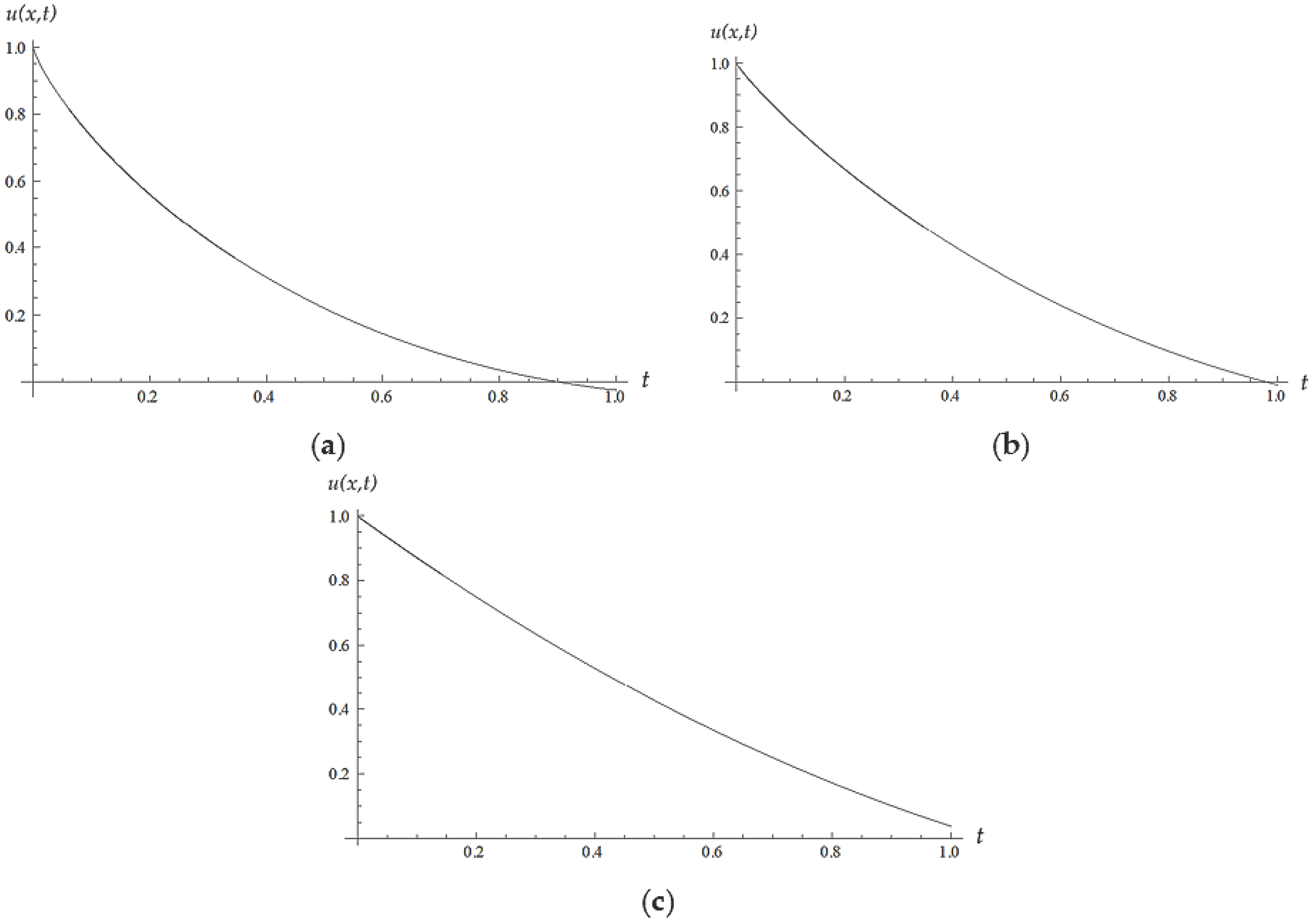
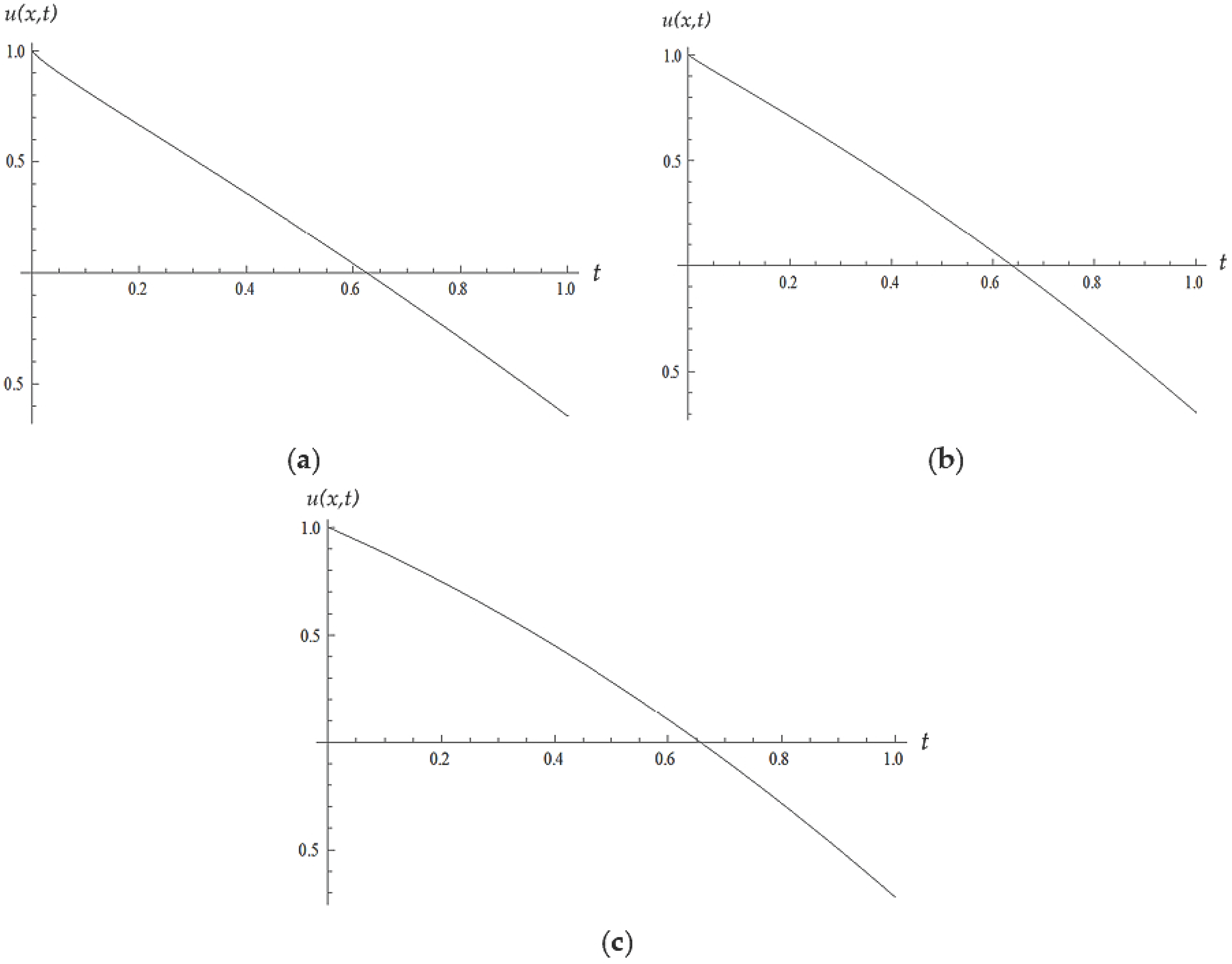
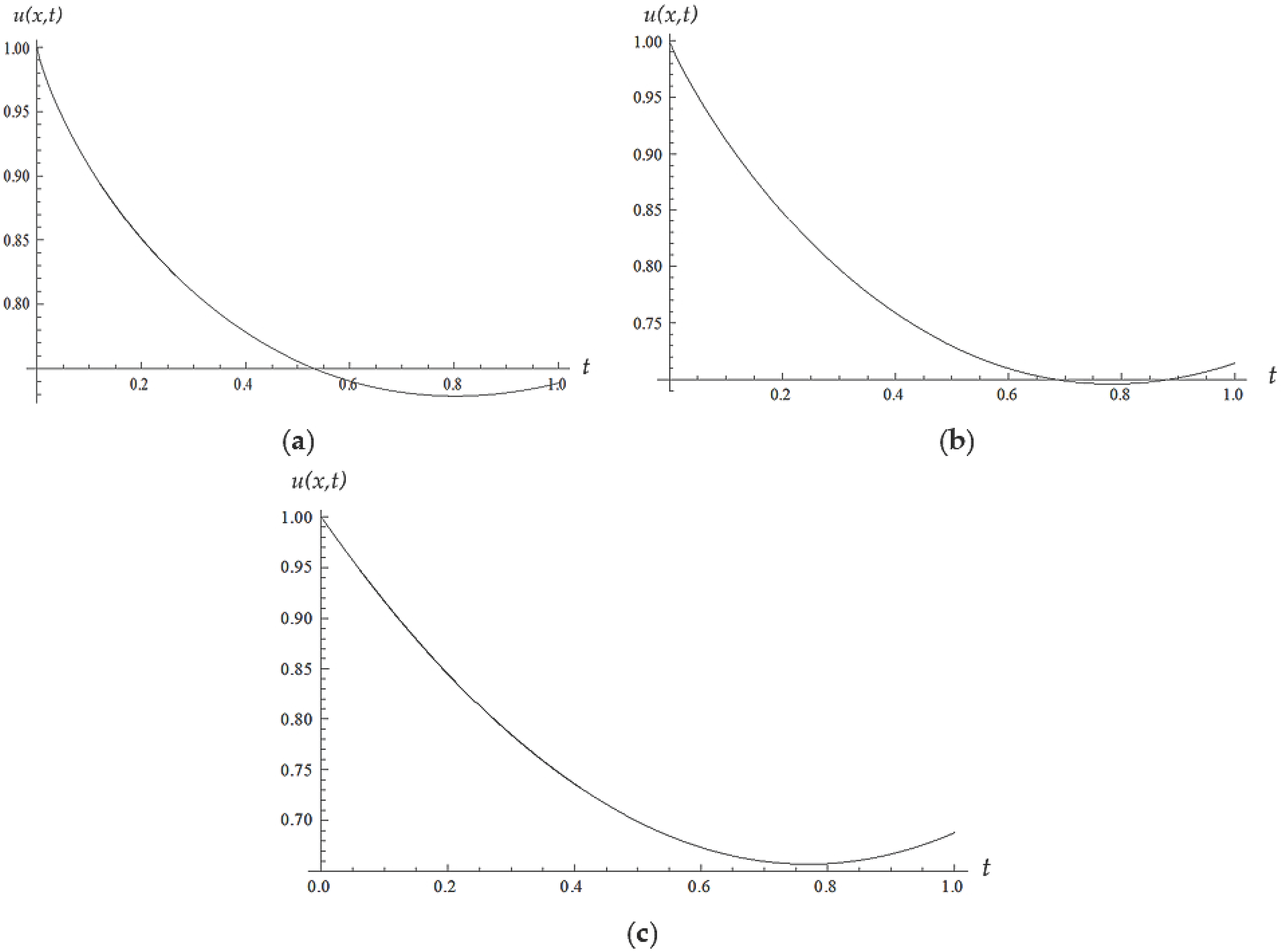
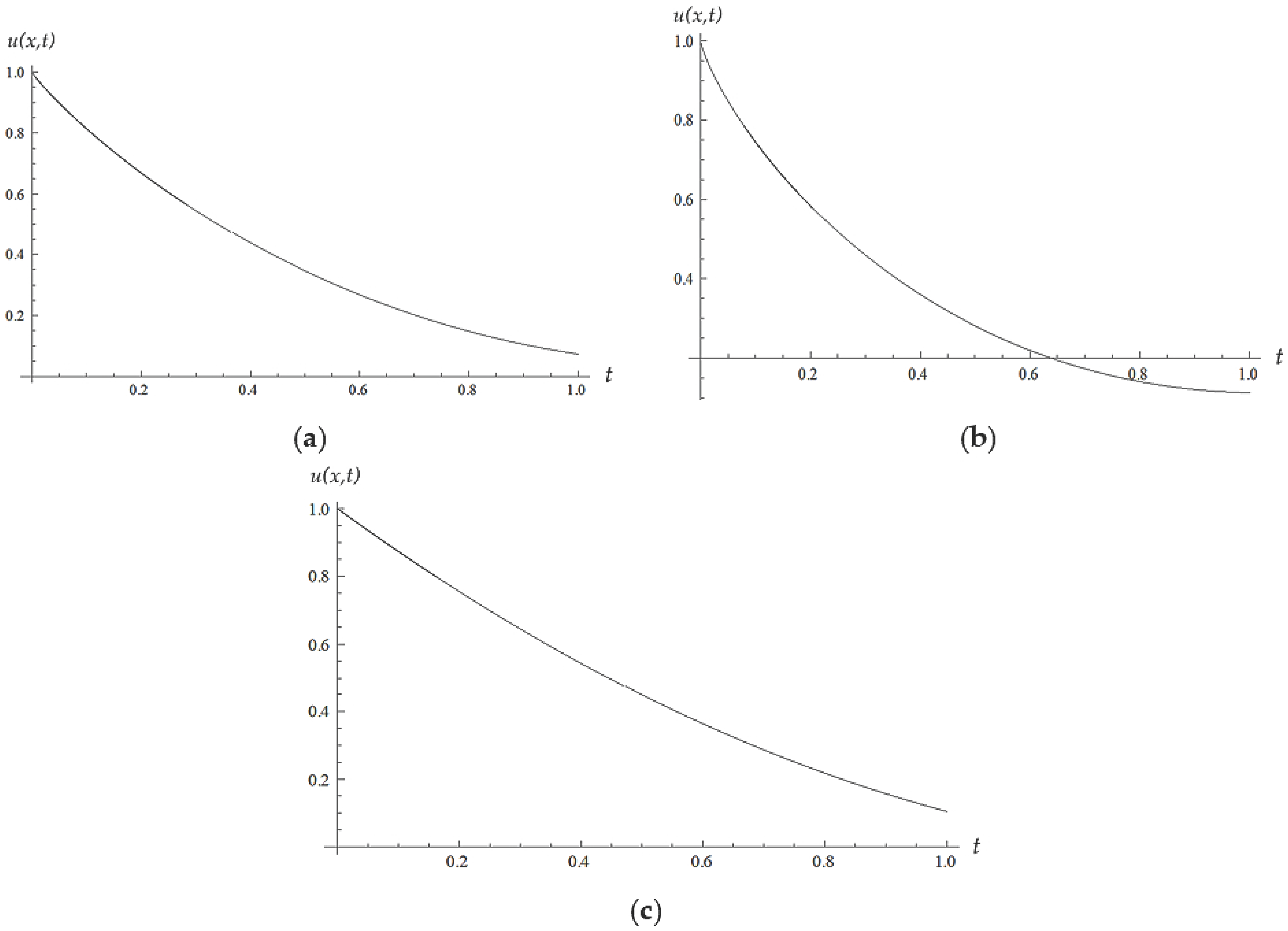
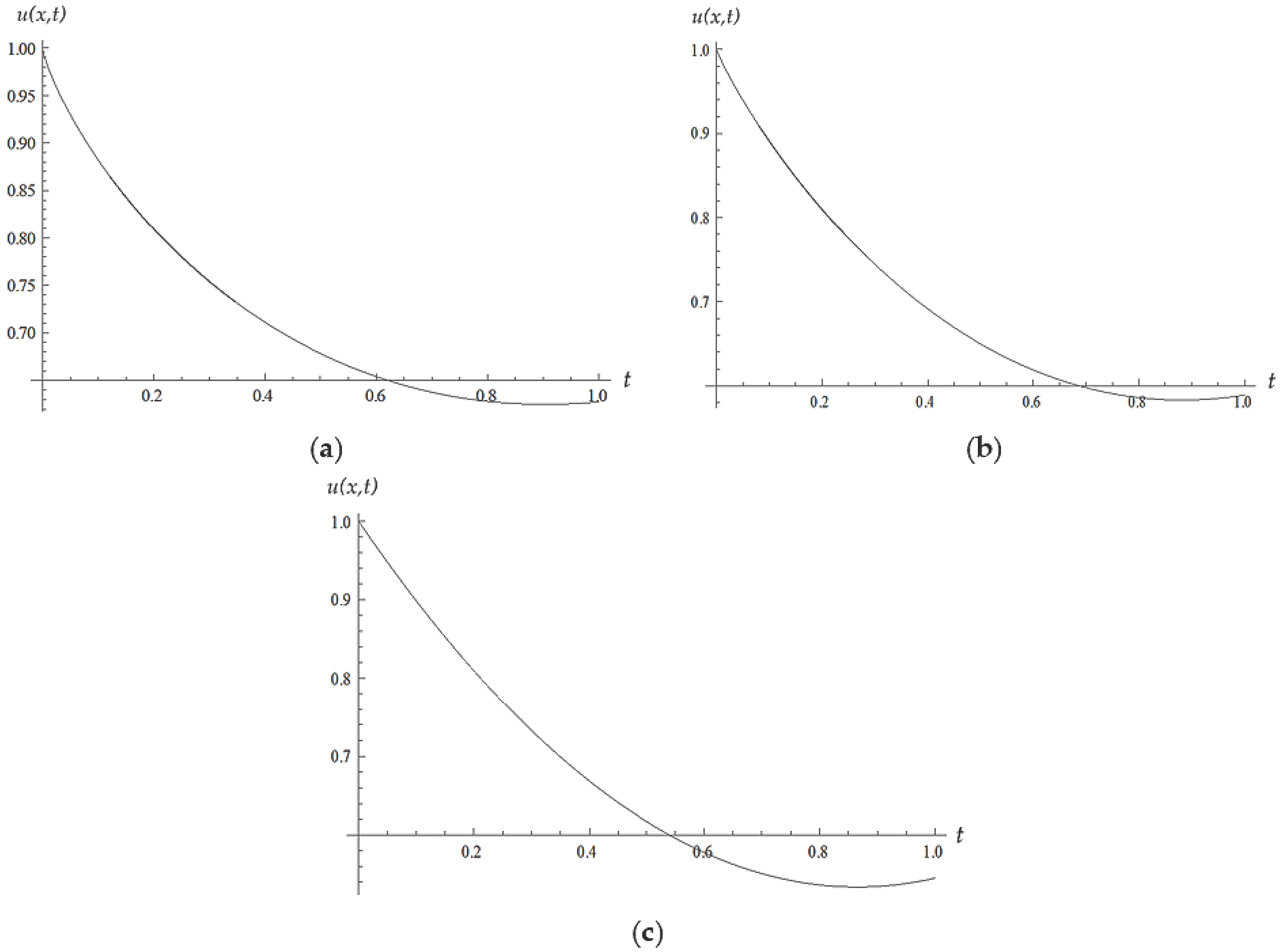
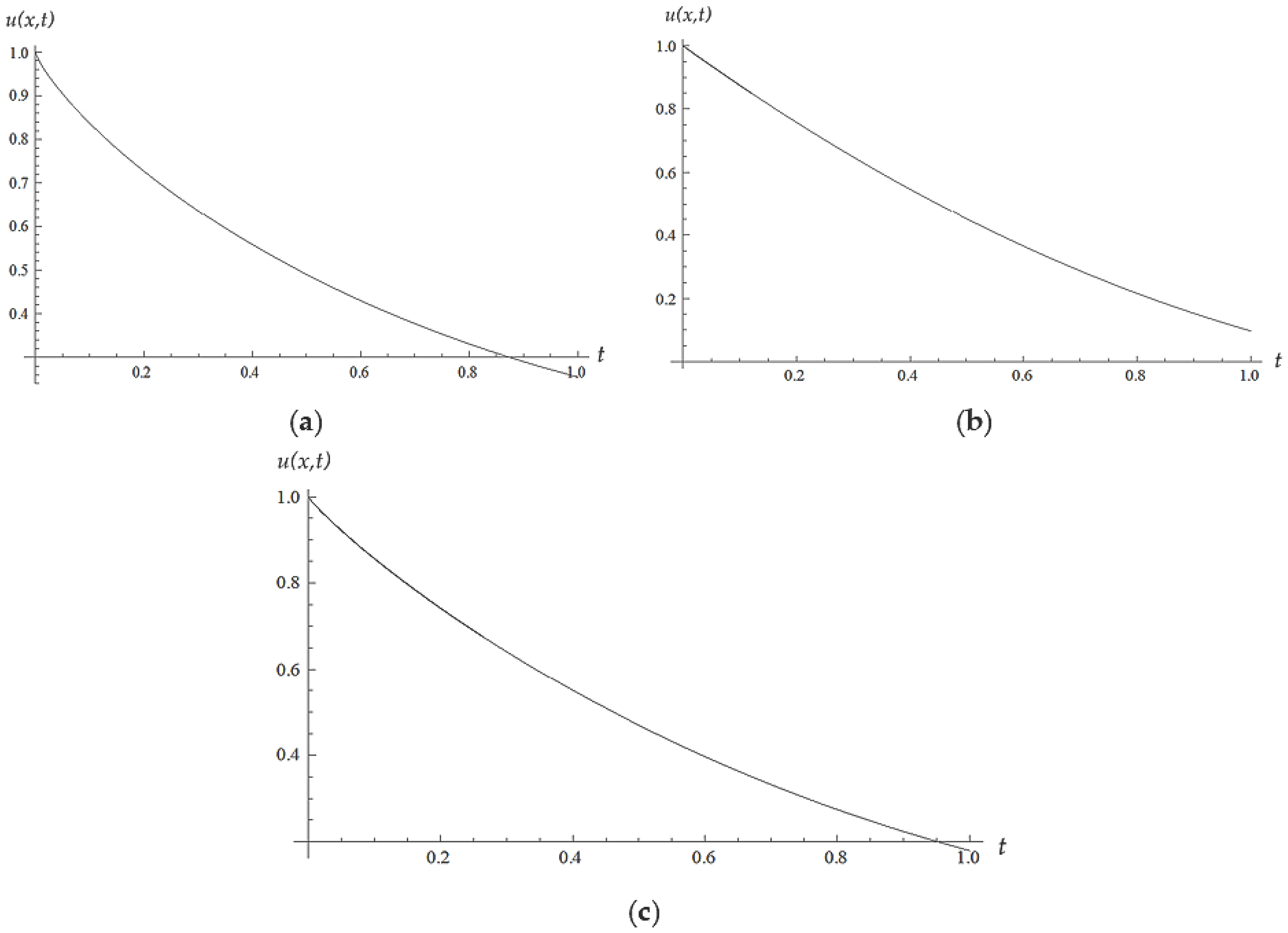
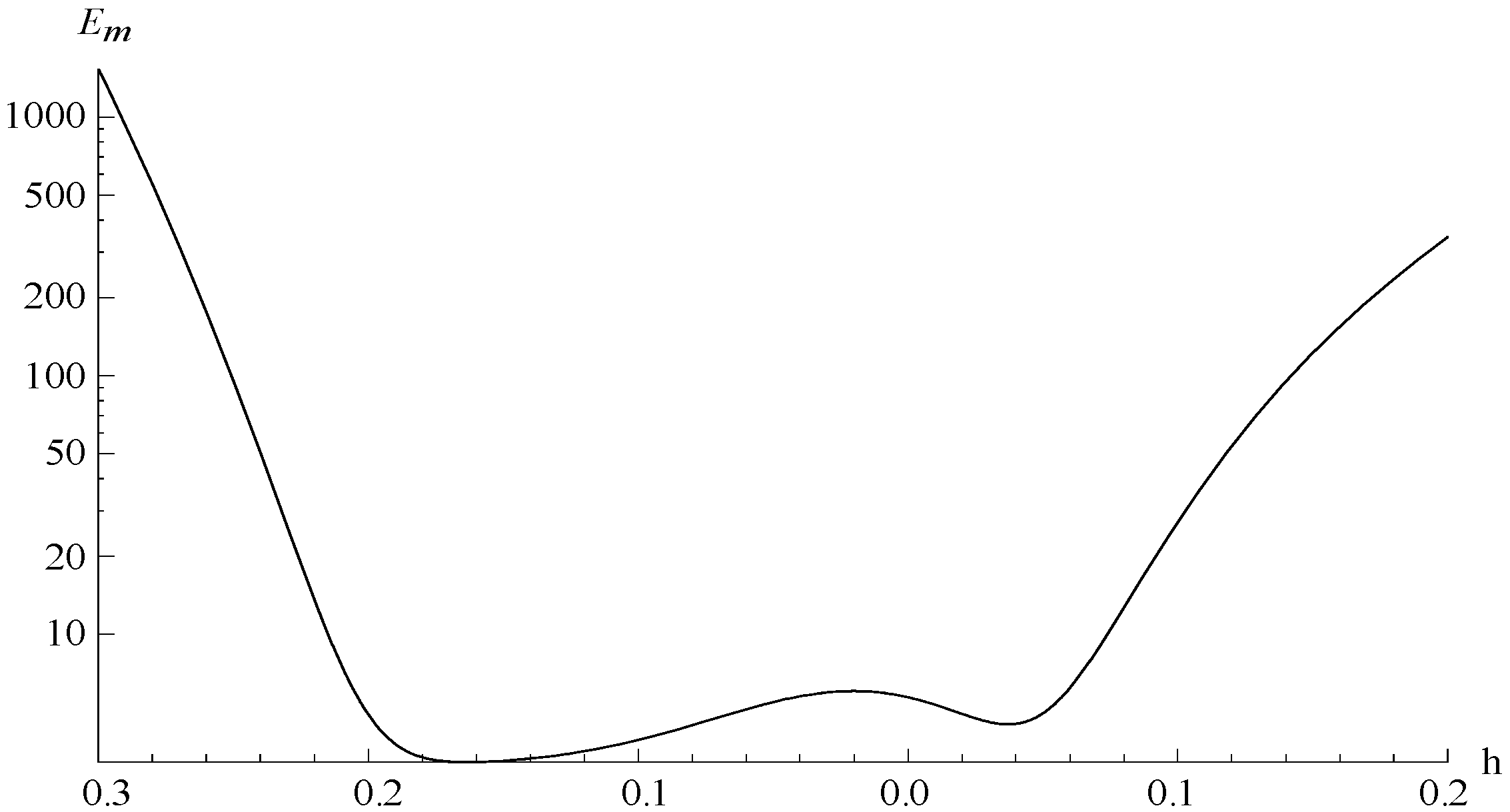
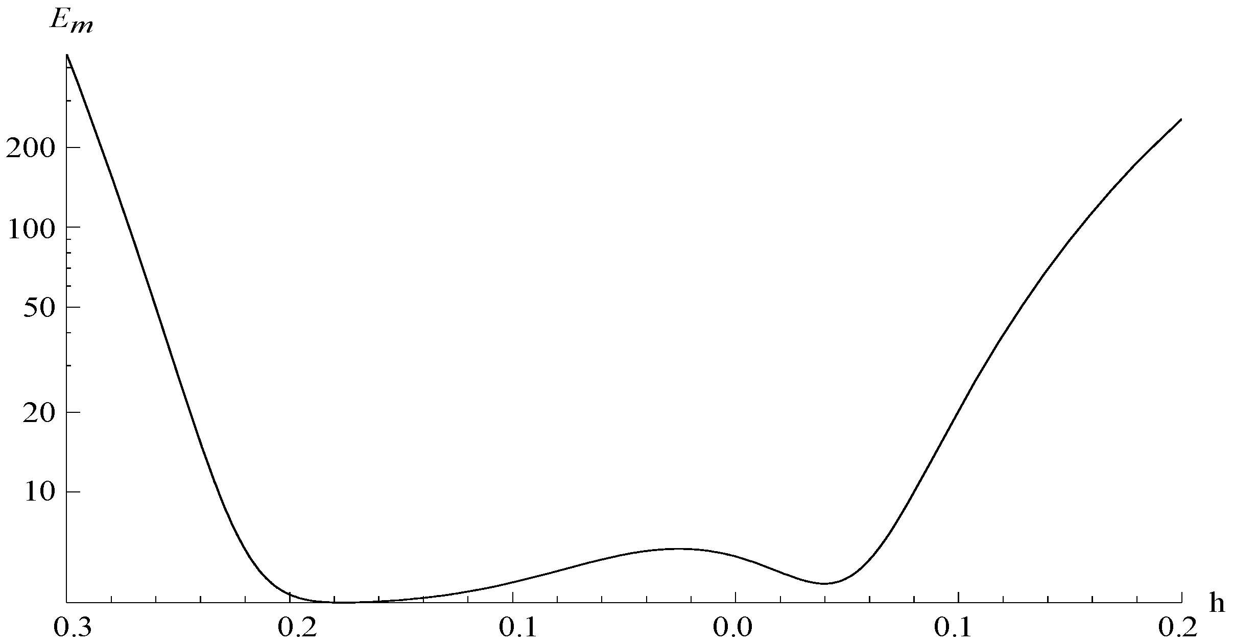
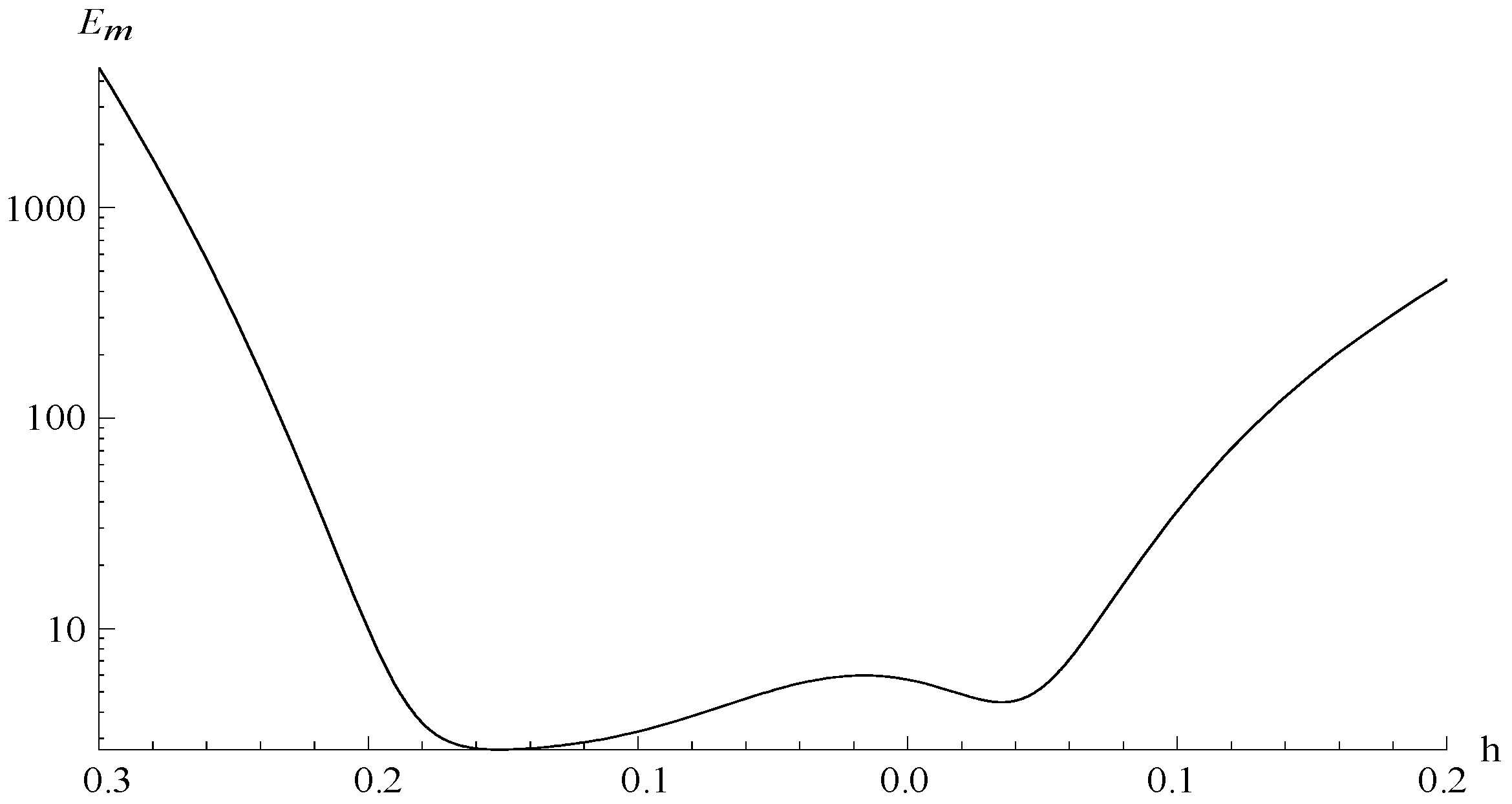
5. Numerical Results and Discussion

In this section, numerical results of the probability density function u(x,t) for different Brownian motion α = 0.8 , 0.9 and also for standard motion α = 1 are calculated for three specific cases: (I) a = b = c = 1 ,   d = 0 , (II) a = b = c = 0 ,   d = 1 and (III) a = b = c = d = 1 .
The variations of u(x,t) vs. t at x = 1 for the above three cases at α = 0.8 , 0.9 , 1.0 are depicted through Figure 1, Figure 2, Figure 3, Figure 4, Figure 5 and Figure 6. During numerical computation, only three terms of the series solution are considered and the accuracy can be increased by introducing more terms in the solution.
It is seen from the Figure 1 that if the diffusivity term is considered as a quadratic polynomial as 1 + u + u 2 , then it is found that u(x,t) decreases with the increases in t and α due to absence, as well as presence, of reaction terms. The rate of decrease is less (Figure 2),when there will be reaction term ( k = 1 ) compared to when there will be no reaction term ( k = 0 ), which reveals that there is the possibility of a highly nonlinear diffusion process to be stabilized for both fractional, as well as standard case, using suitable reaction term.
The nature for the other two considered cases, described through Figure 3, Figure 4, Figure 5 and Figure 6, will be similar. It is also seen from the figures that a decrease of the values of u(x,t) is maximum for the first case and minimum for the third case. This implies that the effect of reaction term will be more if the diffusivity term has quadratic order nonlinearity rather than cubic order nonlinearity.
It is seen from Figure 7, Figure 8 and Figure 9 that the magnitudes of the errors are at a minimum at h = 0.198372 , 0.102184 , 0.17583 for case I, case II, and case III respectively during the presence of reaction term at the standard order case α = 1 taking three terms of the series solutions.

6. Conclusions

The present article has achieved two important goals. The first one is to demonstrate damping of the probability density function, through the use of proper reaction term on the nonlinear diffusion equation, with a diffusivity term consisting of cubic polynomial for different Brownian motion and also for standard motion. The second one is how to accelerate the convergence of approximate solution using the convergence control parameter through error analysis, which reveals the feasibility and the potential of the applied mathematical tool, HAM, during the solution of highly nonlinear partial differential equations in fractional order system. This makes room for future research work where we will study the effect of the advection term in our considered model.

Acknowledgments

The present research work is carried out with the financial support provided by Science & Engineering Research Board (SERB), Government of India. S. Das and S.H. Ong are supported by University of Malaya’s Research Grant Scheme [RP009A-13AFR]. The authors are extending their heartfelt thanks to the revered reviewers for their suggestions towards the improvement of the revised article.

Author Contributions

All authors have contributed equally to the study and preparation of the article. All authors have read and approved the final version of the paper.

Conflicts of Interest

The authors declare no conflict of interest.

Nomenclature

a , b , c , d , k constants
x , t space and time coordinates respectively
u ( x , t ) field variable

Greek Letters

α fractional derivative

References

  1. Zhang, S. Application of Exp-function method to a KdV equation with variable coefficients. Phys. Lett. A 2007, 365, 448–453. [Google Scholar] [CrossRef]
  2. Misirli, E.; Gurefe, Y. Exp-function method to solve the generalized Burgers-Fisher equation. Nonlinear Sci. Lett. A 2010, 1, 1323–1328. [Google Scholar]
  3. Liu, S.; Fu, Z.; Liu, S.; Zhao, Q. Jacobi elliptic function expansion method and periodic wave solutions of nonlinear wave equations. Phys. Lett. A 2001, 289, 69–74. [Google Scholar] [CrossRef]
  4. Yan, Z. Abundant families of Jacobi elliptic function solutions of the (2 + 1)-dimensional integrable Davey-Stewartson-type equation via a new method. Chaos Solitons Fractals 2003, 18, 299–309. [Google Scholar] [CrossRef]
  5. Tascan, F.; Bekir, A.; Koparan, M. Travelling wave solutions of nonlinear evolution equations by using the first integral method. Commun. Nonlinear Sci. Numer. Simul. 2009, 10, 1810–1815. [Google Scholar] [CrossRef]
  6. Abbasbandy, S.; Shirzadi, A. The first integral method for modified Benjamin-Bona-Mahony equation. Commun. Nonlinear Sci. Numer. Simul. 2010, 15, 1759–1765. [Google Scholar] [CrossRef]
  7. Wanga, M.; Lia, X.; Zhanga, J. The ( G G )-expansion method and travelling wave solutions of nonlinear evolution equations in mathematical physics. Phys. Lett. A. 2008, 372, 417–423. [Google Scholar] [CrossRef]
  8. Salas, A.H.; Gomez, C.A. Application of the Cole-Hopf transformation for finding exact solutions to several forms of the seventh-order KdV equation. Math. Probl. Eng. 2010. [Google Scholar] [CrossRef] [PubMed]
  9. Oldham, K.B.; Spanier, J. The Fractional Calculus: Theory and Applications of Differentiation and Integration to Arbitrary Order; Academic Press: Cambridge, MA, USA, 1974. [Google Scholar]
  10. Miller, K.S.; Ross, B. An Introduction to Fractional Calculus and Fractional Differential Equations; John Wiley & Sons: Hoboken, NJ, USA, 1993. [Google Scholar]
  11. Podlubny, I. Fractional Differential Equations; Academic Press: Cambridge, MA, USA, 1999. [Google Scholar]
  12. Liao, S.J. The Proposed Homotopy Analysis Technique for Solution of Nonlinear Problems. Ph.D. Thesis, Shanghai Jiao Tong University, Shanghai, China, 1992. [Google Scholar]
  13. Liao, S.J. Notes on the Homotopy analysis method: Some definitions and theorems. Commun. Nonlinear Sci. Numer. Simul. 2009, 14, 983–997. [Google Scholar] [CrossRef]
  14. Liao, S.J. Beyond Perturbation: Introduction to the Homotopy Analysis Method; CRC Press: Boca Raton, FL, USA, 2003. [Google Scholar]
  15. Liao, S.J.; Cheung, A.T. Application of homotopy analysis method in nonlinear oscillations. ASME J. Appl. Mech. 1998, 65, 914–922. [Google Scholar] [CrossRef]
  16. Liao, S.J. A challenging nonlinear problem for numerical techniques. J. Comput. Appl. Mech. 2005, 181, 467–472. [Google Scholar] [CrossRef]
  17. Liao, S.J.; Cheung, K.F. Homotopy analysis of nonlinear progressive waves in deep water. J. Eng. Math. 2003, 45, 105–116. [Google Scholar] [CrossRef]
  18. Liao, S.J.; Tan, Y. A general approach to obtain series solutions of nonlinear differential equations. Stud. Appl. Math. 2007, 119, 254–297. [Google Scholar] [CrossRef]
  19. Das, S.; Vishal, K.; Gupta, P.K. Solution of the nonlinear fractional diffusion equation with absorbent term and external force. Appl. Math. Model. 2011, 35, 3970–3979. [Google Scholar] [CrossRef]
  20. Das, S. Approximate solution of fractional diffusion equation revisited. Int. Rev. Chem. Eng. 2012, 4, 501–504. [Google Scholar]
  21. Zhang, Y.; Cattani, C.; Yang, X.J. Local Fractional Homotopy Perturbation Method for Solving Non-Homogeneous Heat Conduction Equations in Fractal Domains. Entropy 2015, 17, 6753–6764. [Google Scholar] [CrossRef]
  22. Das, S. Analytical solution of a fractional diffusion equation by variational iteration method. Comput. Math. Appl. 2009, 57, 483–487. [Google Scholar] [CrossRef]
  23. Diethelm, K. The Analysis of Fractional Differential Equation; Springer: Berlin, Germany, 2004. [Google Scholar]
  24. El-Sayed, A.M.A. On the fractional differential equations. Appl. Math. Comput. 1992, 49, 205–213. [Google Scholar] [CrossRef]
  25. Grin’ko, A.P. Solution of a nonlinear differential equation with a generalized fractional derivative. Dokl. Akad. Navnk BSSR 1991, 35, 27–31. [Google Scholar]
  26. Atangana, A. Numerical Analysis of Time Fractional Three Dimensional. Therm. Sci. 2015, 19, 7–12. [Google Scholar] [CrossRef]
  27. Baleanu, D.; Khan, H.; Jafari, H.; Khan, R.A. On the Exact Solution of Wave Equations on Cantor Sets. Entropy 2015, 17, 6229–6237. [Google Scholar] [CrossRef]
  28. Mohyud-Din, S.T.; Iqbal, M.A.; Hassan, S.M. Modified Legendre Wavelets Technique for Fractional Oscillation Equations. Entropy 2015, 17, 6925–6936. [Google Scholar] [CrossRef]
  29. Vishal, K.; Das, S. Solution of the nonlinear fractional diffusion equation with absorbent term and external force using optimal homotopy analysis method. Z. Naturforsch. A 2012, 67, 203–209. [Google Scholar] [CrossRef]
  30. Jafari, H. Numerical Solution of Time-Fractional Klein–Gordon Equation by Using the Decomposition Methods. J. Comput. Nonlinear Dyn. 2016, 11. [Google Scholar] [CrossRef]
  31. Gómez-Aguilar, J.F.; López-López, M.G.; Alvarado-Martínez, V.M.; Reyes-Reyes, J.; Adam-Medina, M. Modeling diffusive transport with a fractional derivative without singular kernel. Physica A 2016, 447, 467–481. [Google Scholar] [CrossRef]
  32. Liu, X.; Lou, B. On a reaction–diffusion equation with Robin and free boundary conditions. J. Differ. Equ. 2015, 259, 423–453. [Google Scholar] [CrossRef]
  33. Morales-Delgado, V.F.; Gómez-Aguilar, J.F.; Yépez-Martínez, H.; Baleanu, D.; Escobar-Jimenez, R.F.; Olivares-Peregrino, V.H. Laplace homotopy analysis method for solving linear partial differential equations using a fractional derivative with and without kernel singular. Adv. Differ. Equ. 2016. [Google Scholar] [CrossRef]
  34. Morgado, M.L.; Rebelo, M. Numerical approximation of distributed order reaction–diffusion equations. J. Comput. Appl. Math. 2015, 275, 216–227. [Google Scholar] [CrossRef]
  35. Gómez-Aguilar, J.F.; Miranda-Hernández, M.; López-López, M.G.; Alvarado-Martínez, V.M.; Baleanu, D. Modeling and simulation of the fractional space-time diffusion equation. Commun. Nonlinear Sci. Numer. Simul. 2016, 30, 115–127. [Google Scholar] [CrossRef]
  36. LenziE, K.; Mendes, G.A.; Mendes, R.S.; Da Silva, L.R.; Lucena, L.S. Exact solutions to nonlinear non-autonomous space-fractional diffusion equations with absorption. Phys. Rev. E 2003, 67, 051109. [Google Scholar] [CrossRef] [PubMed]
  37. Zola, R.S.; Lenzi, M.K.; Evangelista, L.R.; Lenzi, E.K.; Lucena, L.S.; Da Silva, L.R. Exact solutions for a diffusion equation with a nonlinear external force. Phys. Lett. A 2008, 372, 2359–2363. [Google Scholar] [CrossRef]
  38. Mathew, T.P.A. Domain Decomposition Methods for the Numerical Solution of Partial Differential Equations; Springer: Berlin/Heidelberg, Germany, 2008; Volume 61. [Google Scholar]
  39. Gong, C.; Bao, W.; Tang, G.; Jiang, Y.; Liu, J. A Domain Decomposition Method for Time Fractional Reaction-Diffusion Equation. Sci. World J. 2014, 2014, 681–707. [Google Scholar] [CrossRef] [PubMed]
  40. Liao, S. Advances in the Homotopy Analysis Method; World Scientific: Singapore, 2014. [Google Scholar]
Figure 1. Plots of u(x,t) vs. t at x = 1 for a = b = c = 1, d = 0, k = 0: (a) α = 0.8 ; (b) α = 0.9 ; (c) α = 1.0 .
Entropy 18 00329 g001
Figure 2. Plots of u(x,t) vs. t at x = 1 for a = b = c = 1, d = 0, k = 1: (a) α = 0.8 ; (b) α = 0.9 ; (c) α = 1.0 .
Entropy 18 00329 g002
Figure 3. Plots of u(x,t) vs. t at x = 1 for a = b = c = 0, d = 1, k = 0 : (a) α = 0.8 ; (b) α = 0.9 ; (c) α = 1.0 .
Entropy 18 00329 g003
Figure 4. Plots of u(x,t) vs. t at x = 1 for a = b = c = 0, d = 1, k = 1: (a) α = 0.8 ; (b) α = 0.9 ; (c) α = 1.0 .
Entropy 18 00329 g004
Figure 5. Plots of u(x,t) vs. t at x = 1 for a = b = c = d = 1, k = 0: (a) α = 0.8 ; (b) α = 0.9 ; (c) α = 1.0 .
Entropy 18 00329 g005
Figure 6. Plots of u(x,t) vs. t at x = 1 for a = b = c = d = 1, k = 1: (a) α = 0.8 ; (b) α = 0.9 ; (c) α = 1.0 .
Entropy 18 00329 g006
Figure 7. Plots of E m vs. h for case I in the presence of reaction term (k = 1).
Entropy 18 00329 g007
Figure 8. Plots of E m vs. h for case II in the presence of reaction term (k = 1).
Entropy 18 00329 g008
Figure 9. Plots of E m vs. h for case III in the presence of reaction term (k = 1).
Entropy 18 00329 g009

