Study on the Inherent Complex Features and Chaos Control of IS–LM Fractional-Order Systems

Abstract

Based on the traditional IS–LM economic theory, which shows the relationship between interest rates and output in the goods and services market and the money market in macroeconomic. We established a four-dimensional IS–LM model involving four variables. With the Caputo fractional calculus theory, we improved it into a fractional order nonlinear model, analyzed the complexity and stability of the fractional order system. The existences conditions of attractors under different order conditions are compared, and obtain the orders when the system reaches a stable state. Have the detail analysis on the dynamic phenomena, such as the strange attractor, sensitivity to initial values through phase diagram and the power spectral. The order changes in two ways: orders changes synchronously or single order changes. The results show regardless of which the order situation is, the economic system will enter into multiple states, such as strong divergence, strange attractor and the convergence, finally, system will enter into the stable state under a certain order; parameter changes have similar effects on the economic system. Therefore, selecting an appropriate order is significant for an economic system, which guarantees a steady development. Furthermore, this paper construct the chaos control to IS–LM fractional-order macroeconomic model by means of linear feedback control method, by calculating and adjusting the feedback coefficient, we make the system return to the convergence state.

1. Introduction

In recent years, more and more scholars have been paying attention to the changes in the management and economic systems, especially the dynamic characteristics of macro-microeconomic systems. Studies mainly focus on the irregular fluctuations, delay decisions, the changes of the system state, system dynamics, topological structure, etc. [1,2,3]. In the field of theoretical research, scholars mainly focus on the simulation of the nonlinear continuous macro-microeconomic system, and enormous achievements have been made, including the IS–LM model [4,5], van der Pol model [6], Kaldorian model [7] and Goodwin’s accelerated model [8]. The economic system has been extensively studied based on these models. As the study of fractional theory improved gradually, more and more scholars paid attention to the excellent intrinsic characteristics of the fractional-order system, which is widely used in physics, fluid mechanics and random fields in recent years [9,10]. In economics, the limits of integer-order systems become more and more significant, especially under harsh assumptions and it is difficult to reflect on the memory effect of economic variables. Therefore, we select the fractional-order derivation to study the internal complex dynamic characteristics of the macroeconomic system.

At present, the fractional-order research on economic systems is mostly based on the Chen [11,12] system; research interests mainly involve the influence of order change, the stable state, delayed decisions, etc., and the Chen system is a representative model for this. It constructs a 3D macroeconomic dynamics model analyzing the price index (x), investment demand (y) and interest rate (z), simulating the operation process of the macroeconomic system. Besides, the equilibrium points are found, in addition to periodic motion, periodic bifurcation and intermittent chaos. However, the model contains few variables, which leads this model to need optimization.

The IS–LM model is a macroeconomic tool that shows the relationship between interest rates and real output. The intersection of the “investment–saving” (IS) and “liquidity preference–money supply” (LM) curves makes the simultaneous equilibrium in both markets. Based on the analysis above, the classic IS–LM macroeconomics theory is introduced in this paper [13,14,15]. It shows the mutual influence of investment, saving, interest rates, money supply and other factors. Due to the existence of a memory effect of economic variables, we improve the system with the fractional-order theory, and analyze the influence of orders on the system. We present the order of a convergent state, ensuing the stability and controllability of the macroeconomic system. In the field of nonlinear dynamics and chaos control, many scholars have also made great achievements [16,17,18,19,20]; we propose a linear feedback control for the fractional-order IS–LM system, which make the system return to convergence.

2. Construction of the Fractional Order IS–LM Model

2.1. Caputo Fractional Order Derivative Definition and Stability Judgment

At present, there are mainly three definitions of fractional calculus, including the Riemann-Liouville definition, Grünward–Letnikov definition and Caputo definition. In reality, the Caputo calculus definitions can be understood as a weighted integral of the derivative in an interval time, so Caputo calculus has wide application in the fields of physics, fluid mechanics and economic management. The weighted integral gives definition to the differential boundary, so we adopt the Caputo fractional calculus definition in this paper.

Definition. 

Caputo fractional differential: For any nonnegative real number α, n–1 ≤ α < n a continuous function f(t): R⁺ → R as a function which is defined in the interval [a, b] (a, b is finite or ∞), then:

$$\begin{array}{ll}{}_a{}^{C}D_t^{\alpha }f(t):& =\frac{d^n}{d{t}^n}{}_{\alpha }D_t^{-(n-\alpha )}f(t)\\ & =\{\begin{array}{l}\frac{1}{\Gamma (n-\alpha )}{\displaystyle {\int }_a^t\frac{f^{(n)}(\tau )}{{(t-\tau )}^{\alpha +1-n}}d\tau , n-1<\alpha <n,}\\ \frac{d^n}{d{t}^n}f(t), \alpha =n\end{array}\end{array}\forall t\in [a,b]$$

is called the left Caputo derivative in α order, denoted as: $D_t^{\alpha }f(t)$, where Γ is the Γ-function: $\Gamma (n-\alpha )={\displaystyle {\int }_0^{\infty }{e}^{-t}{t}^{n-\alpha -1}dt}$, $\Gamma (\alpha +1)=\alpha \Gamma (\alpha )$.

The Stability of Fractional Order System

Compared with traditional integer order systems, although the fractional order calculus system has the same equilibrium point, the stability condition of equilibrium point is completely different. Based on previous research [21] we know that for fractional order systems, even if the real part of the eigenvalues is positive, the system may still be in a stable state.

Lemma 1. 

Sufficient condition for the convergence of equilibrium point E:

Autonomous System $D_t^{\alpha }x(t)=A(x)$, $x(0)=x_0$ is asymptotically stable if and only if:

$$\underset{i}{\text{min}}\left|\text{arg}(eig{(A)}_i)\right|>\text{max}\left[\raisebox{1ex}{$\alpha \pi $}\!\left/ \!\raisebox{-1ex}{$2$}\right.\right]$$

(1)

At this time, the variable shows convergence with the Mittag-Leffler α.

Lemma 2. 

Necessary condition for the system to enter into chaos:

$$\underset{i}{\text{min}}\left|\text{arg}(eig(A))\right|\le \underset{i}{\text{min}}\left[\raisebox{1ex}{$\alpha \pi $}\!\left/ \!\raisebox{-1ex}{$2$}\right.\right]$$

(2)

Lemma 1 is the sufficient condition for asymptotic stability of the equilibrium point; Lemma 2 is the necessary condition for the system to enter into chaos.

2.2. Economics Meaning of Caputo Fractional Derivative

In recent years, there have been numerous applications of fractional-order calculus in various fields. Economic dynamics is a new interdisciplinary area among them, which is commonly applied to describe internal complexity of financial and economic problems. We show a concrete example to illustrate the memory effect of economic variables.

For the investment demand $I(t)$, $I^{(m)}(t)$ is its integer order derivative, and $D_0^{q}I(t)$ can be regarded as the corresponding fractional order derivative. At the time $t$, $I^{(m)}(t)$ indicates the m-th order change ratio of the investment demand, and it is only related to the time $t$, having nothing to do with the time before, that is, in integer order derivatives, there is no memory effect in economic variables; However, the fractional order derivation $D_0^{q}I(t)$ is the weighted integral of all m-th orders on the whole interval $[0,t]$, the derivation $D_0^{q}I(t)$ is not only related to time $t$, but also related to any time before $t$, so fractional order derivation has the capacity to reflect the memory effect of economic variables.

A large number of economic variables have memory effects, so in the actual economic analysis, fractional differential has very important practical significance. In this paper, in order to better reflect on the memory effect of economic variables and study the complex dynamic characteristics of the economic system, we have introduced the Caputo fractional derivative to the traditional IS–LM model.

2.3. Four-Dimensional IS–LM Macroeconomics Model

The traditional IS–LM model is two-dimension macroeconomics model. With the continuous development of theory, the four-dimensional IS–LM model gradually formed and the concept of variable price was introduced [14], which has a simulation effect on the actual running state of the product market and money market. The dynamics of macroeconomics require full time complete and highly accurate modeling.

In the case of a pure money financing deficit, we assume that the macroeconomics system is:

$$\{\begin{array}{ll}\stackrel{•}{Y(t)}=& {\alpha }_1[I(Y(t),R(t))+g-s(Y^D(t))-T(t)]\\ & +{\alpha }_2[R(t)+cP(t)-1]Y(t)\\ \stackrel{•}{R(t)}=& {\beta }_{1}P(t)+{\beta }_2[L(Y(t),R(t))-M(t)]\\ \stackrel{•}{P(t)}=& 1-R(t)-cP(t)+\gamma [g-\nu Y(t)]\\ \stackrel{•}{M(t)}=& g-\nu Y(t)\end{array}$$

(3)

where $Y$ is the national income; $I$ is investment; $g$ is government expenditures (constant); $s$ is savings; $T$ is tax revenue; $R$ is interest rate; $L$ is capital turnover; $M$ is real currency supply quantity, $Y^D(t)$ is the pure national income, that is $Y^D(t)=Y(t)-T(T)$, $c$ is the cost parameter, ${\alpha }_i,{\beta }_i(i=1,2)$ are positive parameters.

From IS–LM model (3), we know clearly that the first equation describes traditional disequilibrium adjustment in the product market; compared with the traditional model that is described the well-known works of Schinasi [22,23], this paper considers the influence of national income in this period to the next, that is ${\alpha }_2[R(t)+cP(t)-1]Y(t)$, where ${\alpha }_2$ is the influence. The second equation describes the disequilibrium dynamic adjustment in the money market. The third equation describes average commodity prices in the market; this equation is not shown in the traditional IS–LM model. Average commodity prices have a direct relationship with interest rates, government expenditures and national income. The fourth equation describes the government’s budget constraint, only in the form of money in case finance deficits.

Besides, from [2] we know that investment, capital turnover, saving and tax revenue meet the following conditions:

$$\{\begin{array}{l}I(Y(t),R(t))=aY{(t)}^{k_1}R{(t)}^{-k_2}\\ L(Y(t),R(t))=mY(t)+\raisebox{1ex}{$r_1$}\!\left/ \!\raisebox{-1ex}{$(R(t)-r_2)$}\right.\\ s(Y^D(t))=s(1-\nu )Y(t)\\ T(t)=\nu Y(t)\end{array}$$

(4)

In the investment process, investment $I$ is positively correlated with income $Y(t)$; negatively correlated with interest rates $R(t)$, the correlation being of exponential form. In this paper, we describe investment of the economic model by $aY{(t)}^{k_1}R{(t)}^{-k_2}$. In product market, the national income is decided by the level of aggregate demand which is composed by the consumption, investment, government expenditures and net exports, the investment demand is subject to the interest rate, the interest rate is determined by the supply and demand of the currency market, that is, the product market is affected by the currency market. On the other hand, the national income has an impact on currency supply quantity, and affects the market interest rate, that is, the currency market is affected by the product market, and the price factor is an indispensable variable within economic analysis, which directly reflect the changes in inflation, interest rates, volume of currency and other economic indicators, so the analysis of the price index combined with the IS–LM model is of practical significance.

3. Theoretical Analysis of Fractional Order IS–LM System

Combining Equations (3) with Equations (4), and performing a fractional transform, we have the fractional order four-dimensional economic system:

$$\{\begin{array}{ll}{D}_t^{q_1}Y(t)=& {\alpha }_1[aY{(t)}^{k_1}R{(t)}^{-k_2}+g-s(1-\nu )Y(t)-\nu Y(t)]\\ & +{\alpha }_2[R(t)+cP(t)-1]Y(t)\\ D_t^{q_2}R(t)=& {\beta }_{1}P(t)+{\beta }_2[mY(t)+\raisebox{1ex}{$r_1$}\!\left/ \!\raisebox{-1ex}{$(R(t)-r_2)$}\right.-M(t)]\\ D_t^{q_3}P(t)=& 1-R(t)-cP(t)+\gamma [g-\nu Y(t)]\\ D_t^{q_4}M(t)=& g-\nu Y(t)\end{array}$$

(5)

where $s\in (0,1)$, $a,k_1,k_2,m,r_1,r_2,\nu >0$.

The fractional-order system is non-local, which brings about great difficulty for its numerical solution, the traditional Euler discrete and Runge–Kutta methods are no longer suitable for fractional-order systems. In this paper, we take a predictor-corrector scheme to discretize the fractional IS–LM economic system.

Let $(Y_0,R_0,P_0,M_0)$ be the initial point of the system, the discrete time step is $h=T/N,t_n=nh,n=0,1,\dots ,N\in Z^{+}$.

Then through the Volterra integral equation, the system can be rewritten as the following form with equivalent transformation of predictor-corrector scheme, as shown in [24]:

$$\begin{array}{ll}{Y}_{n+1}=Y_0& +\frac{h^{q_1}}{\Gamma (q_1+2)}{\alpha }_1\left[a{\left(Y_{n+1}^p\right)}^{k_1}{\left(R_{n+1}^p\right)}^{-k_2}+g-s(1-\nu )Y_{n+1}^p-\nu Y_{n+1}^p\right]\\ & +\frac{h^{q_1}}{\Gamma (q_1+2)}{\alpha }_2\left(R_{n+1}^p-c{P}_{n+1}^p-1\right)Y_{n+1}^p\\ & +\frac{h^{q_1}}{\Gamma (q_1+2)}{\displaystyle \sum _{j=0}^n{\alpha }_{1,j,n+1}\left[a{Y_j}^{k_1}{R_j}^{-k_2}+g-s(1-\nu )Y_j-\nu Y_j\right]}\\ & +\frac{h^{q_1}}{\Gamma (q_1+2)}{\displaystyle \sum _{j=0}^n{\alpha }_{1,j,n+1}}{\alpha }_2\left(R_j-c{P}_j-1\right)Y_j\end{array}$$

$$\begin{array}{ll}{R}_{n+1}=R_0& +\frac{h^{q_2}}{\Gamma (q_2+2)}\left[{\beta }_1{P}_{n+1}^p+{\beta }_2\left(m{Y}_{n+1}^p+\frac{r_1}{R_{n+1}^p-r_2}-M_{n+1}^p\right)\right]\\ & +\frac{h^{q_2}}{\Gamma (q_2+2)}{\displaystyle \sum _{j=0}^n{\alpha }_{2,j,n+1}}\left[{\beta }_1{P}_j+{\beta }_2\left(m{Y}_j+\frac{r_1}{P_j-r_2}-M_j\right)\right]\end{array}$$

$$\begin{array}{ll}{P}_{n+1}=P_0+& \frac{h^{q_3}}{\Gamma (q_3+2)}\left[1-R_{n+1}^p-c{P}_{n+1}^p+\gamma \left(g-\nu Y_{n+1}^p\right)\right]\\ & +\frac{h^{q_3}}{\Gamma (q_3+2)}{\displaystyle \sum _{j=0}^n{\alpha }_{3,j,n+1}}\left[1-R_j-c{P}_j+\gamma \left(g-\nu Y_j\right)\right]\end{array}$$

$$M_{n+1}=M_0+\frac{h^{q_4}}{\Gamma (q_4+2)}\left(g-\nu Y_{n+1}^p\right)+\frac{h^{q_4}}{\Gamma (q_4+2)}{\displaystyle \sum _{j=0}^n{\alpha }_{4,j,n+1}}\left(g-\nu Y_j\right)$$

where:

$$\begin{array}{ll}{Y}_{n+1}^p=Y_0+& \frac{1}{\Gamma (q_1)}{\displaystyle \sum _{j=0}^n{\beta }_{1,j,n+1}{\alpha }_1\left(a{Y_j}^{k_1}{R_j}^{-k_2}+g-s(1-\nu )Y_j-\nu Y_j\right)}\\ & +\frac{1}{\Gamma (q_1)}{\displaystyle \sum _{j=0}^n{\beta }_{1,j,n+1}}{\alpha }_2\left(R_j-c{P}_j-1\right)Y_j\end{array}$$

$$R_{n+1}^p=R_0+\frac{1}{\Gamma (q_2)}{\displaystyle \sum _{j=0}^n{\beta }_{2,j,n+1}}\left[{\beta }_1{P}_j+{\beta }_2\left(m{Y}_j+\frac{r_1}{P_j-r_2}-M_j\right)\right]$$

$$P_{n+1}^p=P_0+\frac{1}{\Gamma (q_3)}{\displaystyle \sum _{j=0}^n{\beta }_{3,j,n+1}}\left[1-R_j-c{P}_j+\gamma \left(g-\nu Y_j\right)\right]$$

$$M_{n+1}^p=M_0+\frac{1}{\Gamma (q_4)}{\displaystyle \sum _{j=0}^n{\beta }_{4,j,n+1}}\left(g-\nu Y_j\right)$$

Parameters ${\alpha }_{i,j,n+1},{\beta }_{i,j,n+1}(i=1,2,3,4)$ are respectively:

$${\alpha }_{i,j,n+1}=\{\begin{array}{ll}{n}^{q_i+1}-(n-n^{q_i}){(n+1)}^{q_i}& j=0\\ {(n-j+2)}^{q_i+1}+{(n-j)}^{q_i+1}-2{(n-j+1)}^{q_i+1}& 1\le j\le n\\ 1& j=n+1\end{array}$$

$$\begin{array}{cc}{\beta }_{i,j,n+1}=\frac{h^{q_i}}{q_i}\left[{(n-j+1)}^{q_i+1}-{(n-j)}^{q_i+1}\right]& 0\le j\le n\end{array}$$

Errors of this method: $\underset{j=1,2,\dots ,N}{\text{max}}\left|f(t_j)-f_h(t_j)\right|=o(h_p)(i=1,2,3,4)$, where: $f=Y,R,P,M$, $p_i=\text{min}(2,1+q_i)$, $(i=1,2,3,4)$.

3.1. Equilibrium Solution and Its Stability of the System

In order to analyze the running state of the fractional-order IS–LM macroeconomic system, we need to analyze the stability of its equilibrium points. We can easily know the macroeconomic IS–LM system (5) has just one equilibrium point $\left(Y_0(t),R_0(t),P_0(t),M_0(t)\right)$, where:

$$Y_0(t)=\frac{g}{\nu }; R_0(t)={\left(\frac{a{Y}_0^{k_1-1}}{s(1-\nu )}\right)}^{\frac{1}{k_2}};$$

$$P_0(t)=\frac{1-R_0}{c}; M_0(t)=m{Y}_0+\frac{r_1}{(R_0-r_2)}+\frac{{\beta }_1}{{\beta }_2}{P}_0$$

According to the practice, the equilibrium must larger than 0, which is:

$$\left(Y_0(t),R_0(t),P_0(t),M_0(t)\right)>0$$

Therefore, calculate and we can get:

$$\frac{ag}{\nu }<s(1-\nu )$$

In actual simulation and analysis, the parameters must meet this condition.

The Jacobi matrix of the system (5):

$$J=\left(\begin{array}{cccc}{l}_{11}& l_{12}& {\alpha }_{2}cY(t)& 0\\ {\beta }_{2}m& -r_1{\left[R(t)-r_2\right]}^{-2}& {\beta }_1& -{\beta }_2\\ -\gamma \nu & -1& -c& 0\\ -\nu & 0& 0& 0\end{array}\right),$$

where:

$$l_{11}={\alpha }_{1}a{k}_{1}Y{(t)}^{k_1-1}R{(t)}^{-k_2}-s(1-\nu )-\nu +{\alpha }_2\left[R(t)+cP(t)-1\right]$$

$$l_{12}={\alpha }_{1}aY{(t)}^{k_1}(-k_2)R{(t)}^{-k_2-1}+{\alpha }_{2}Y(t)$$

Calculate the eigenvalues of the system (5):

$$P(\lambda )={\lambda }^4+a_1{\lambda }^3+a_2{\lambda }^2+a_3\lambda +a_4$$

(6)

where:

$$a_1=s(1-\nu )+\nu -{\alpha }_{1}a{k}_{1}Y{(t)}^{k_1-1}R{(t)}^{-k_2}-{\alpha }_2\left[R(t)+cP(t)-1\right]+c+r_1{[R(t)-r_2]}^{-2}$$

$$\begin{array}{ll}{a}_2=& (c+{\beta }_1)r_1{[R(t)-r_2]}^{-2}+\left(s(1-\nu )+\nu -{\alpha }_{1}a{k}_{1}Y{(t)}^{k_1-1}R{(t)}^{-k_2}-{\alpha }_2[R(t)+cP(t)-1]\right)\\ & \left(c+r_1{[R(t)-r_2]}^{-2}\right)+\left({\alpha }_{1}aY{(t)}^{k_1}{k}_{2}R{(t)}^{-k_2-1}+{\alpha }_{2}Y(t)\right)\left(-{\beta }_{2}m\right)+{\alpha }_{2}cY(t)\gamma \nu \end{array}$$

$$\begin{array}{ll}{a}_3=& \left(s(1-\nu )+\nu -{\alpha }_{1}a{k}_{1}Y{(t)}^{k_1-1}R{(t)}^{-k_2}-{\alpha }_2\left[R(t)+cP(t)-1\right]\right)(c+{\beta }_1)r_1{[R(t)-r_2]}^{-2}\\ & +\left({\alpha }_{1}aY{(t)}^{k_1}{k}_{2}R{(t)}^{-k_2-1}+{\alpha }_{2}Y(t)\right)\left(-{\beta }_{2}mc-{\beta }_2\nu +{\beta }_1\gamma \nu \right)\\ & +{\alpha }_{2}cY(t)\left({\beta }_{2}m+\gamma \nu r_1{[R(t)-r_2]}^{-2}\right)\end{array}$$

$$a_4=-{\beta }_2\nu c\left[{\alpha }_{1}aY{(t)}^{k_1}{k}_{2}R{(t)}^{-k_2-1}-{\alpha }_{2}Y(t)\right]+{\alpha }_{2}cY(t)\nu {\beta }_2$$

Through numerical simulation, we can obtain the eigenvalues of the system, then combined with Lemma 1: $\underset{i}{\text{min}}\left|\text{arg}(eig{(A)}_i)\right|>\text{max}\left[\raisebox{1ex}{$\alpha \pi $}\!\left/ \!\raisebox{-1ex}{$2$}\right.\right]$, we can determine the commensurate order of the system when the system is stable, that is, the macroeconomics system gradually evolve, and enter into stable state eventually in this order condition. The system is controllable and forms a good macroeconomic operation trend.

3.2. Dissipativity and the Existence of Attractor

In the chaos theory, the dissipative degree is an important index to determine whether the nonlinear system is convergent to the attractor. In this paper, we adopt the following approach to calculate the dissipativity of the system, and determine whether the system converges to the attractor:

$$\nabla V=\frac{\partial \left(\raisebox{1ex}{$d^{q_1}Y$}\!\left/ \!\raisebox{-1ex}{$d{t}^{q_1}$}\right.\right)}{\partial Y}+\frac{\partial \left(\raisebox{1ex}{$d^{q_2}R$}\!\left/ \!\raisebox{-1ex}{$d{t}^{q_2}$}\right.\right)}{\partial R}+\frac{\partial \left(\raisebox{1ex}{$d^{q_3}P$}\!\left/ \!\raisebox{-1ex}{$d{t}^{q_3}$}\right.\right)}{\partial P}+\frac{\partial \left(\raisebox{1ex}{$d^{q_4}M$}\!\left/ \!\raisebox{-1ex}{$d{t}^{q_4}$}\right.\right)}{\partial M}$$

(7)

Obviously, (7) is the trace of Jacobi matrix, so $\nabla V$ of system (5) is:

$$\begin{array}{ll}\nabla V=& {\alpha }_{1}a{k}_{1}Y{(t)}^{k_1-1}R{(t)}^{-k_2}-s(1-\nu )-\nu \\ & +{\alpha }_2\left[R(t)+cP(t)-1\right]-r_1{\left[R(t)-r_2\right]}^{-2}-c\end{array}$$

(8)

when $\nabla V<0$, system (5) dissipates with a contraction rate $e^{\nabla V}$, which means the trajectories of the chaotic system (5) converge onto an attractor ultimately. The dissipation or the convergence of the system depends entirely on the symbol of $\nabla V$. We can verify the existence of attractor in theory system through the calculation of dissipativity in different order conditions.

4. Analysis on Dynamic Evolution of Fractional Order IS–LM System

With the numerical simulation of the system (5), we set parameters:

$$\begin{array}{l}a=0.37,{\alpha }_1=0.95,{\alpha }_2=0.65,k_1=0.39,k_2=0.92,m=0.0015,\nu =0.0585\\ s=0.25,{\beta }_1=0.9,{\beta }_2=0.92,r_1=0.5,r_2=0.9,c=0.1788,\gamma =0.01,g=0.001\end{array}$$

After calculation, we can get the initial value of the system (5) is:

$$(Y_0=0.04,R_0=0.066,P_0=1\times {10}^{-6},M_0=0.025)$$

Analyze the operation state of the system under the integer-order condition: that is $q=q_1=q_2=q_3=q_4=1$.

According to (8), we can compute $\nabla V$ of the system: $\nabla V=-0.3864<0$, under the parameter conditions (7), the trajectories of system will gradually gathered to attractor in speed of $e^{-0.3864}$.

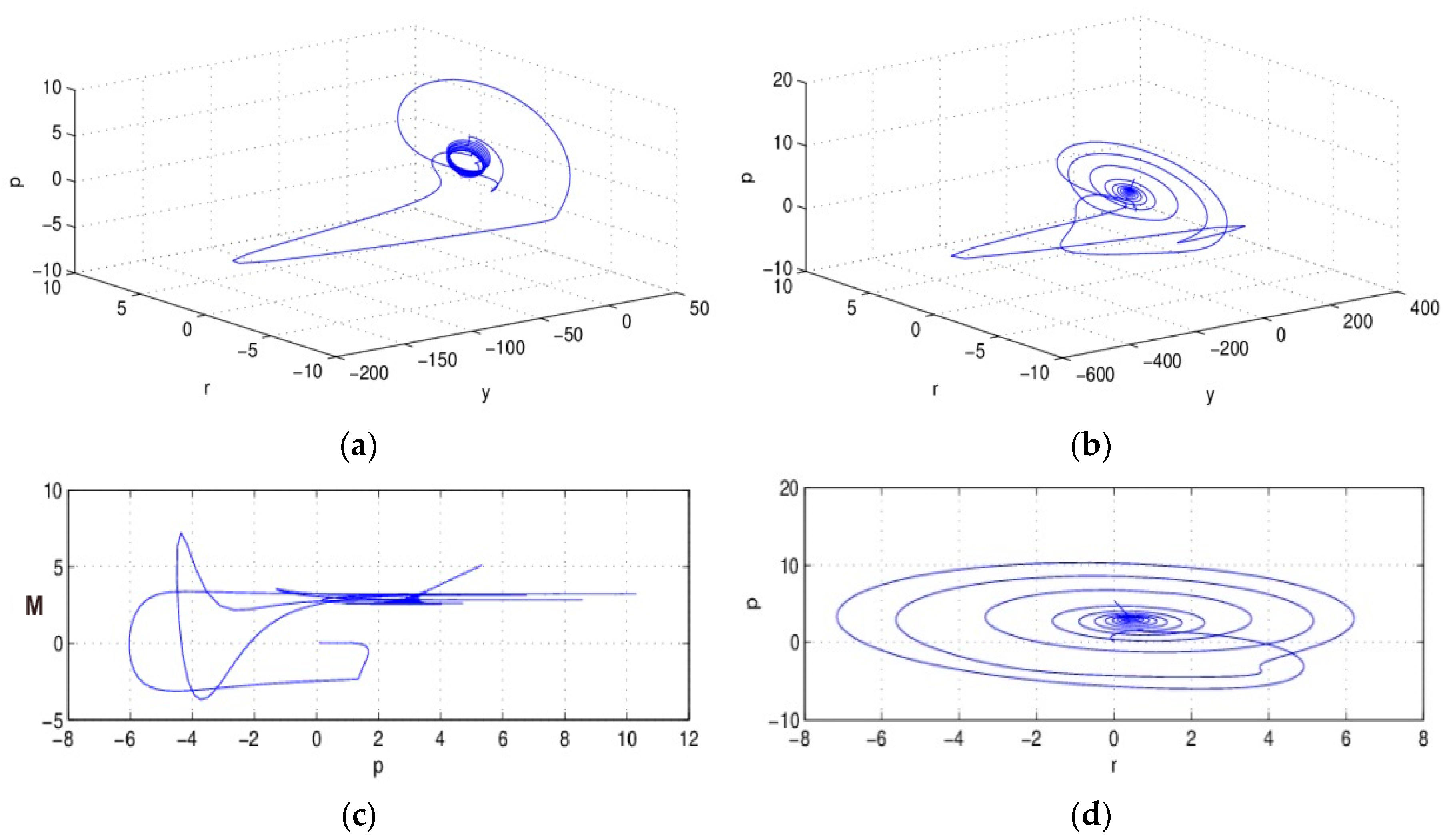
Under the condition of integer-order, when $q=q_1=q_2=q_3=q_4=1$, the attractor of system (5) is shown in Figure 1.

From Figure 1, we find that the IS–LM system (5) gathered to the attractor, and formed periodic motion under the integer order condition $q=q_1=q_2=q_3=q_4=1$. Figure 1c,d are the projections of the system in plane P-M and P-R; we notice that after initial evolution, the system converges to the attractor gradually, and presents regularity of movement. The attractor is the characteristic of a chaos system, which means the macro-economic system (5) is in chaos state under the condition of $q=1$, and a small variation of the initial conditions of the system will lead to enormous differences in the results, and this is not acceptable in the actual economic system.

4.1. Commensurate Order Case

When $q=q_1=q_2=q_3=q_4$ gradually decreases from 1 to 0, the system (5) shows a different dynamic evolution state, transitioning gradually from intense divergence to convergence, as shown in Figure 2.

From Figure 2, we find that with $q_1=q_2=q_3=q_4$ gradually decreased from 1 to 0 synchronously, the operation state of the system changes too. When $q=1$, the trajectory of the system converges to the attractor gradually, and forms a cyclic solution; When $q<1$, that the system just entered into (0, 1), and the system shows strong divergence; this phenomenon should not be allowed in the actual macroeconomic system; this situation continues until $q=0.8$, from Figure 2b, where we notice that the system gradually converges, the macroeconomics are stable, and can be controlled, which is the state we were hoping to see. With the further decrease of $q$, the system no longer converges, and enters into normal operation conditions. This situation continues until the convergence condition.

Convergent State of the System

According to Lemma 1, we obtain the convergence condition when $q=q_1=q_2=q_3=q_4$.

The eigenvalue of the system is ${\lambda }_{1,2}=-0.2084\pm 0.0532i$; ${\lambda }_{3,4}=0.01517\pm 0.0661i$, we found that the real part of ${\lambda }_{3,4}$ is larger than 0, so the equilibrium point $E(Y_0,R_0,P_0,M_0)$ is unstable, based on $\left|\text{arg}(eig{(A)}_i)\right|>\text{max}\left[{\alpha }_i\pi /2\right]$, the order condition when the system converges can be obtained, that is $q_i<0.1593$; all variables of the system gradually converge.

When $q=q_1=q_2=q_3=q_4=0.15$, the running state of each variable is shown in Figure 3.

As shown in Figure 3, when $q=q_1=q_2=q_3=q_4=0.15<0.1593$, each variable enters into the stable state gradually, the fractional order economic system shows convergence, stability and controllability.

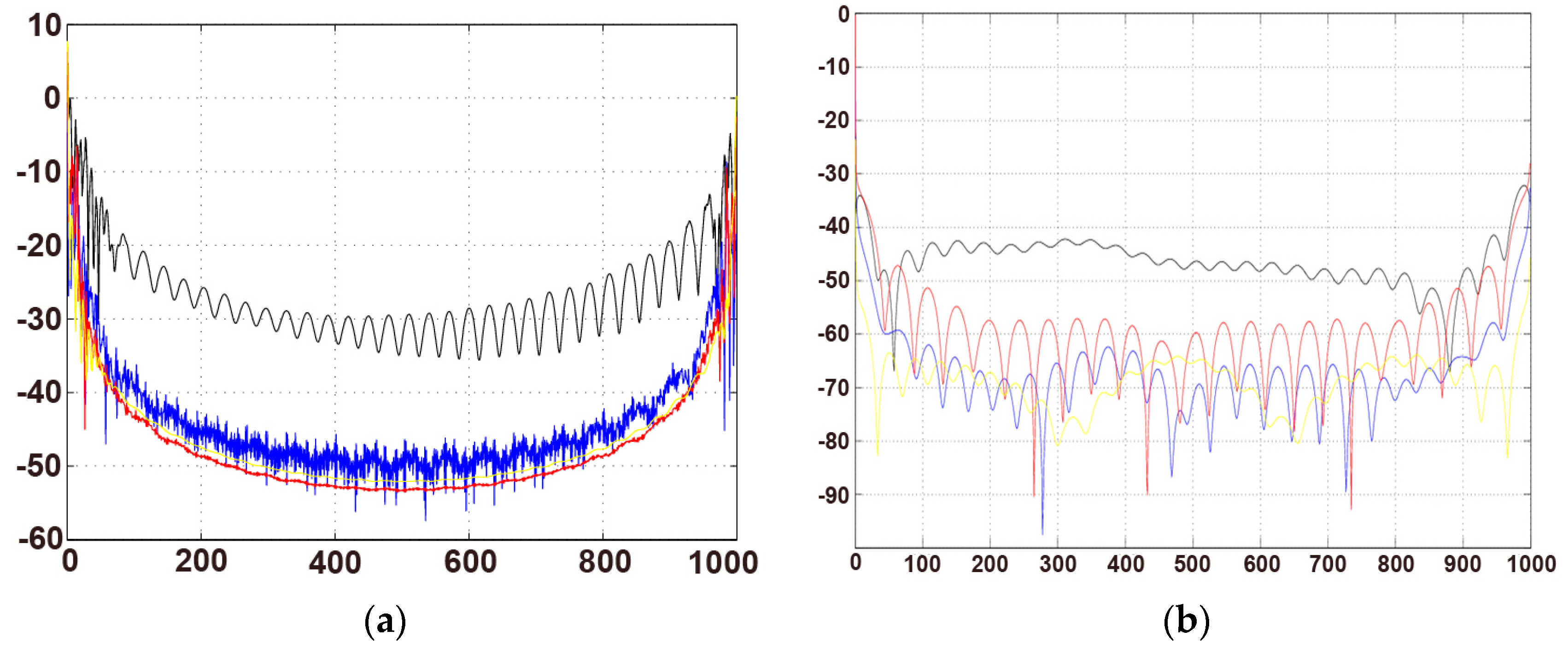
The power spectrum is one of important tools to describe the running state of the system; we can judge the chaos situation from the spectrum shape. When $q=q_1=q_2=q_3=q_4=1$ and 0.15, the power spectrum is shown in Figure 4.

As we know, the power spectrum is one of the features for distinguishing the chaotic state of the system, and is also an important method to study the system entering into chaos from bifurcation. In the power spectrum, periodic motion appears as a peak and chaotic situations appear as “background noise”. From Figure 4 we find the change clearly. The system in Figure 4a is in a noise background, and changing to the peak state gradually in Figure 4b.

4.2. Incommensurate Order Case

While the order of the system changes incommensurately, due to the many variables contained in the four-dimensional macroeconomics system, this paper only discusses the influence of single order changes on the system running state.

(1)

$q_2=q_3=q_4=1$, and $q_1$ changes, the state changes of system (5) are shown in Figure 5.

From Figure 5, we found that when $q_2=q_3=q_4=1$, and $q_1$ reduces from 1 to 0, the running state of system (5) changed gradually, when $q_1=0.999$, the system still converges to the attractor, but the scope of activities of the attractor decreases slightly relative to $q=q_1=q_2=q_3=q_4=1$; When $q_1=0.995$, the system (5) converges, suggesting that the economy system reaches the stable development state, this shows that by single change of $q_1$, the IS–LM macro-economic system realizes the convergent state, and the system goes back to a controllable state from a chaos state. Continuous decreases of $q_1$ brought about different states to the system, but the system finally returns to the stable operation state, the steady development of the economic system, which is in accordance with its normal development situation.

(2)

When $q_2,q_3,q_4$ change separately, the state change of system (5) is shown in Figure 6. Similar to the change state of $q_1$, when $q_1=q_3=q_4=1$, and $q_2$ reduces from 1 to 0, from Figure 6a–d, the running state of system (5) changes gradually. When $q_2=0.999$, the system began to converge from the attractor, that is, the system convergence just entered the fractional order state, the four-dimensional macroeconomics system running stably, and under controlled conditions.

With the reduction of $q_2$, when $q_2=0.97$, the system is in a state of strong divergence, which should be avoided in the actual process; when $q_2=0.95$, the system is back to the convergence condition again, and the economic system back to a controllable situation; When $q_2$ reduces to 0.905 gradually, the system gradually converges to a chaotic attractor, and forms a periodic solution.

The system appears in a similar situation when $q_3,q_4$ change separately, as shown in Figure 6e–h, which shows that order changes in a single dimension have an important impact on the running state of the system (5), the system appears in several running state such as strong divergence, forming the attractor, convergence, which have an important influence on the economic system. To ensure the stable and healthy development of the economic system, we should try to select the suitable order which leads the system to enter into a convergence state, and must avoid the system going into a strongly divergent state. We find that, with the fractional order reduction, the system will appear in similar running state as “divergence, attractors and convergence”, but these several situations have no obvious sequence rules, just like with the reduction of $q_1$, the system first enters into an attractor state, then changes into convergent and strongly divergent states; meanwhile, with the reduction of $q_2$, the system converges first, then shows strong divergence, after that the system goes back to a convergent state, then enters into an attractor state; similar “no obvious sequence rules” status also occur in the changing process of $q_3,q_4$. Therefore in the actual economic system operation process, we should choose the order of the system appropriately, to ensure the convergence of system (5).

4.3. Chaos Control of IS–LM Fractional-Order System

The chaos situation has a huge influence on the the nonlinear system, especially economic systems, so in the macroscopic readjustment and control, the economic system should be prevented from entering into the chaotic state by the government and central bank. Generally, the chaos control methods of fractional-order systems are similar to those of integer-order systems. In this section, we select the appropriate feedback intensity factor through the linear feedback control method to realize the stability or periodic solution of the chaotic system.

According to the eigenvalues of the system (5) ${\lambda }_{1,2}=-0.2084\pm 0.0532i$; ${\lambda }_{3,4}=0.01517\pm 0.0661i$, the equilibrium point of the system is unstable. Adding the linear feedback to the system (5), the linear feedback system changes into:

$$\{\begin{array}{ll}{D}_t^{q_1}Y(t)=& {\alpha }_1[aY{(t)}^{k_1}R{(t)}^{-k_2}+g-s(1-\nu )Y(t)-\nu Y(t)]\\ & +{\alpha }_2[R(t)+cP(t)-1]Y(t)+l_1\left[Y(t)-Y_0\right]\\ D_t^{q_2}R(t)=& {\beta }_{1}P(t)+{\beta }_2[mY(t)+\raisebox{1ex}{$r_1$}\!\left/ \!\raisebox{-1ex}{$(R(t)-r_2)$}\right.-M(t)]\\ & +l_2\left[R(t)-R_0\right]\\ D_t^{q_3}P(t)=& 1-R(t)-cP(t)+\gamma [g-\nu Y(t)]+l_3\left[P(t)-P_0\right]\\ D_t^{q_4}M(t)=& g-\nu Y(t)+l_4\left[M(t)-M_0\right]\end{array}$$

(9)

where, $l_i(i=1,2,3,4)$ are the feedback intensity factors, $E(Y_0,R_0,P_0,M_0)$ is the equilibrium point of the system. Select the appropriate feedback intensity factor, make $l=l_1=l_2=l_3=l_4$. We can calculate that when $l>3.7$, the coefficients of the characteristic equation at the equilibrium point are: $a_1=-8.107$, $a_2=-8.032$, $a_3=-7.918$, $a_4=1.972$. 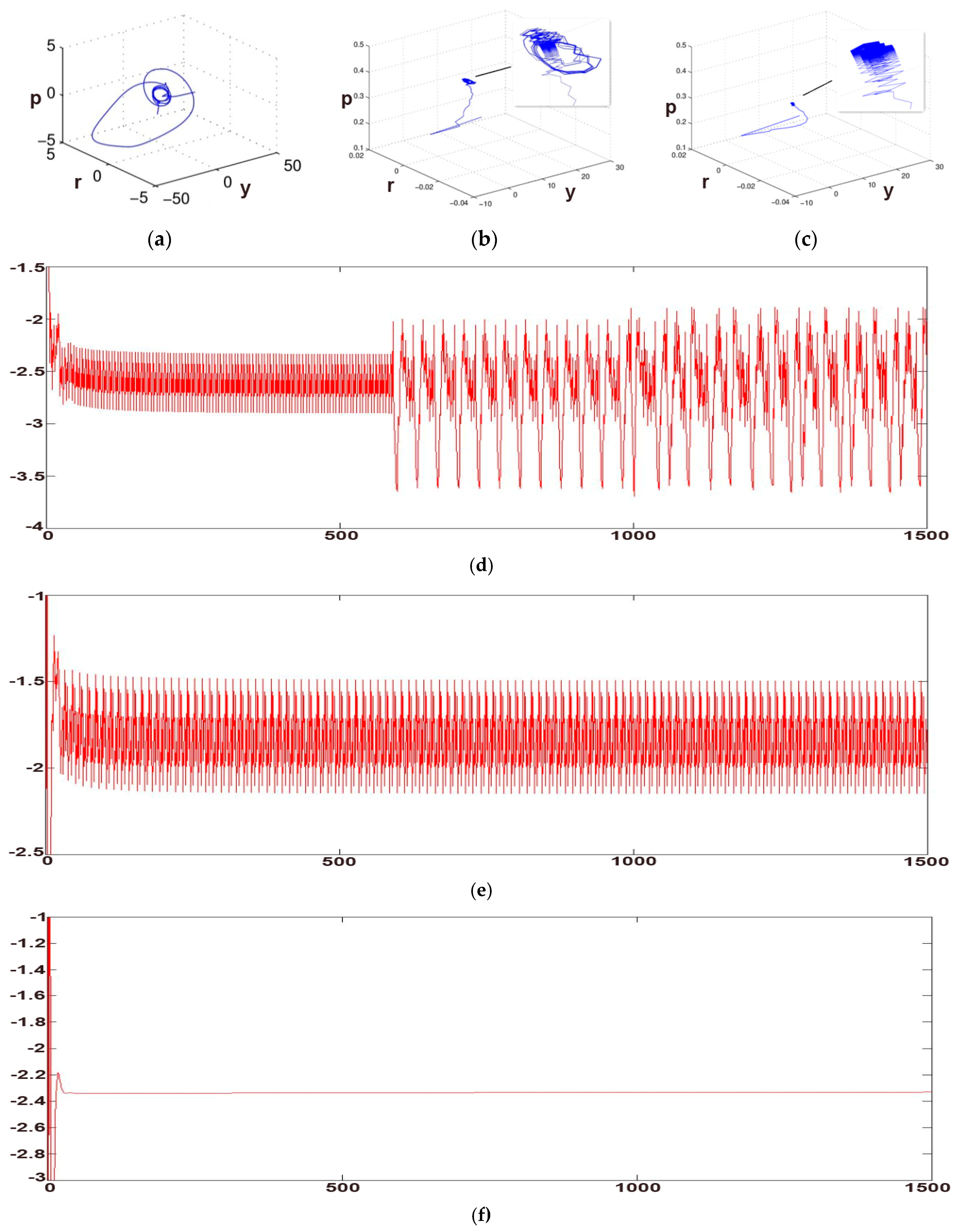According to the Routh-Hurwitz condition of fractional order systems, the system will be stable on the equilibrium point E. The phrase diagram and variable $Y(t)$ changes when $l=2,2.5,4$ as shown in Figure 7.

As can be seen from Figure 7, when the order of the system $q=(0.99,0.95,0.89,0.9)$, the running state of the system is shown in Figure 7a, and the system forms a chaotic attractor, and it is not convergent. This state is not desirable for macroeconomic systems. At this point, we consider the feedback intensity factor $l$, and have chaos control in the system. According to the analysis above, we know that the system goes back to convergence when $l>3.7$; and when $l=2$, the system is in a divergent state, which can be seen in Figure 7b,d; and when $l=2.5$, the system gradually converges and forms the attractor, which can be seen in Figure 7c we can also notice this phenomenon in Figure 7e, national income $Y(t)$ forms an attractor; when $l$ gradually increased to $l=4$, the system enters into the convergence state, as shown in Figure 7f, at this moment; the chaos state of the system is well controlled.

In the actual macroeconomic system, it is difficult for the system to appear in full accordance with the status of the integer order system; most of the situations are in accordance with the fractional order system. This shows that the fractional order system is universal in actual macroeconomics. Therefore under this condition, extended analysis of the economic system through the theory of fractional order, and study under the condition of economic operation of the system has important significance, through the analysis of the change speed of the system on the stability of the whole economic system, and then analysis of the government's economic policy has important practical significance.

5. Conclusions

In recent years, many studies have focused on the situation and the structure of economic systems under complex dynamic theory conditions. This paper aims at the IS–LM macroeconomics model and improves it with the fractional-order theory, guaranteeing the memory characteristics of the variables in a macroeconomic system. With the definition of Caputo fractional calculus, we carried out an approximate simulation to the IS–LM model.

We calculate the equilibrium point and get a sufficient condition of orders when the system reaches a steady state, deriving the corresponding parameters. Then we analyze and observe the operation state of the system through numerical simulation in two ways: the first is when the orders change synchronously, the second is single order changes. Simulation results show that the state changes a lot in the operation process. We present the power spectrum of the system to provide some evidence of the change state of the system. Under the condition of fractional order, the system may enter into a chaotic state, and in view of this situation, this paper proposes chaos control by means of a linear feedback control method. The results show that when the feedback parameters $l>3.7$, the system returns to a stable state.

Numerical simulation results show that regardless of which kind of situation the order is, the economic system will enter into multiple states, such as strong divergence, strong attractor and the convergence, and finally, the system will enter into the stable state under a certain order; parameter changes have similar effects on the economic system. With fractional order theory, we can achieve the stability of the macroeconomic system with no change to the variables and parameters. In a real macroeconomics system, it is important to prevent the system from entering into a chaotic state, and it is essential to ensure the system is controllable.