Determining the Entropic Index q of Tsallis Entropy in Images through Redundancy

Abstract

The Boltzmann–Gibbs and Tsallis entropies are essential concepts in statistical physics, which have found multiple applications in many engineering and science areas. In particular, we focus our interest on their applications to image processing through information theory. We present in this article a novel numeric method to calculate the Tsallis entropic index q characteristic to a given image, considering the image as a non-extensive system. The entropic index q is calculated through q-redundancy maximization, which is a methodology that comes from information theory. We find better results in the image processing in the grayscale by using the Tsallis entropy and thresholding q instead of the Shannon entropy.

1. Introduction

Image segmentation is a fundamental stage in image processing, which consists of dividing an image in regions with common characteristics, for example separating the object from the background. There is a great variety of segmentation procedures, as is shown in [1], and it is a previous stage of the image classification. Due to its easier implementation and low requirement of CPU resources [2], image segmentation by thresholding based on gray level histogramming is the most intuitive and common approach, and it is performed as follows: for a given image, the thresholding consists of finding a gray threshold level, so it can allow the histogram division in two sets; the less than or or equal levels to this threshold will be zero, and the greater than gray levels will be one. This process changes the original image into a binary image. In this procedure, there are several ways to find the optimal threshold to separate the image into two sets. The methods described in [2,3,4,5] explain image segmentation procedures based on the Shannon and Tsallis entropy. Particularly, in [6], a nonextensive information theoretic divergence was proposed called Jensen–Tsallis divergence; in [7], image registration is carried out by maximizing a Tsallis entropy-based divergence using a modified simultaneous perturbation stochastic approximation algorithm. However, in such examples and many more, the entropic index q is chosen “by eye”.

The Boltzmann–Gibbs entropy and the Tsallis entropy [8,9] are essential concepts in statistical physics. Recently, in [9], it has been shown how the dynamics of the standard map exhibits the crossing from the Tsallis and Boltzmann–Gibbs statistics. In statistical physics, there has been a concerted research effort to explore the properties of Tsallis entropy, leading to a statistical mechanics that satisfies many of the properties of the standard theory [6]. These entropies have found multiple applications in many engineering and science areas [10,11,12], such as in the image processing through information theory [5,13,14]. The Tsallis entropy is a generalization of the Boltzmann–Gibbs entropy. The Tsallis approach entropy considers the systems as non-extensive, which are characterized by the entropic index q [10,15]. Although for certain particular cases, methods to calculate q are well known [10,11], there does not exist a general methodology to estimate q for a given system (physical, biological, economical, etc.). In the case of our interest, when images are processed with the Tsallis entropy, also there is not a general method to know the entropic index q, which is a characteristic parameter of the image, and it is usually estimated in an empiric way [5,13].

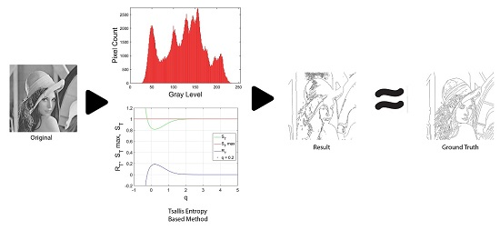
Our main goal here is to provide a methodology to calculate the entropic index q based on the maximization of the image redundancy and the maximum entropy principle of information theory. An image is considered as a system with information that can be measured; this can be Shannon or Tsallis entropy information. Redundancy, information and maximum entropy can also be measured in a given system. When these concepts are applied in images, the entropic index q can be estimated. Finally, in order to implement our methodology, it is necessary to implement a segmentation image procedure based on the Shannon and Tsallis thresholding procedure [5,13,16]. A better segmentation and edge detections are obtained when the images are considered as non-extensive systems with their entropic index q previously calculated, so we show that in image processing, Tsallis entropy is better than Shannon entropy.

In Section 2 of this paper, a brief and general review of Boltzmann–Gibbs and Tsallis physical entropies is given, along with corresponding information theory analogies. In Section 3, we explain our methodology to calculate the entropic index q and segmenting the images. Then, in Section 4, an explanation of the digital processing image using entropy is given, to emphasize the gray level picture thresholding using the Tsallis entropy of the histogram. Results and the corresponding discussion are presented in Section 5. Finally, a brief summary is given in Section 6. The Supplementary Materials present a step by step resume of all procedures and algorithms used to calculate the Shannon and Tsallis entropies of our images.

2. Boltzmann–Gibbs and Tsallis Entropy

In thermodynamics, at the end of the 19th century, Ludwig Boltzmann [10] proposed the following entropy definition:

$$S_B=k\ln \left(\mathsf{\Omega }\right)$$

(1)

where $k=1.3806504\times {10}^{-23}$J·K${}^{-1}$ is Boltzmann’s constant and Ω represents the total number of accessible microstates of the system. Equation (1) is essential in classical statistical physics. This entropy is a particular case where all microstates probabilities are the same, i.e., $p_i=1/\mathsf{\Omega },\forall i$. Nevertheless, if these probabilities are not the same, then Equation (1) is generalized to Boltzmann–Gibbs entropy, given by:

$$S_{BG}=-k\sum _{i=1}^{\mathsf{\Omega }}{p}_i\ln \left(p_i\right)$$

(2)

For each i, where $p_i$ satisfies the normalization condition:

$$\sum _{i=1}^{\mathsf{\Omega }}{p}_i=1$$

(3)

In fact, $S_{BG}$ is maximum when the microstates are equiprobable, i.e., $p_i=1/\mathsf{\Omega },\forall i$, as a consequence $S_{BG\max }=S_B=k\ln \left(\mathsf{\Omega }\right)$.

In 1988, Tsallis proposed a new kind of entropy [8], able to describe extensive and non-extensive systems, defined as:

$$S_T=\frac{k}{q-1}\left(1-\sum _{i=1}^{\mathsf{\Omega }}{p}_i^q\right)$$

(4)

where Ω represents the total number of accessible microstates of the system, each one with probability $p_i$, where $(1\le i\le \mathsf{\Omega })$ and probabilities $p_i$ satisfy Equation (3). The number $q\in \mathbb{R}$ is an entropic index that characterizes the degree of non-extensivity of the system [10,17]. It is used to describe systems with non-extensive properties, and it is also used to characterize the non-extensivity degree of a particular system. A system is considered extensive if it satisfies the equation $S_{BG}(A+B)=S_{BG}\left(A\right)+S_{BG}\left(B\right)$; it is non-extensive if it does not.

The Tsallis entropy has four important properties [18]:

• When ${\lim }_{q\to 1}{S}_T$ the Boltzmann–Gibbs entropy $S_{BG}$ is recovered; this can be proven by using the L′Hôpital theorem. Then $S_T$ is a generalization of $S_{BG}$, i.e., the non-extensive statistical physics includes Boltzmann–Gibbs statistical physics as a particular case.
• $S_T$ is zero only when some $p_i=1$.
• Pseudo-extensivity or non-extensivity of $S_T$. Let A and B be two independent systems in the probability theory sense, i.e., $p_{ij}^{A+B}=p_i^A+p_j^B$, $\forall ij$, then the next equation can be verified:

  $$S_T(A+B)=S_T\left(A\right)+S_T\left(B\right)+\frac{1-q}{k}{S}_T\left(A\right)S_T\left(B\right)$$

  (5)
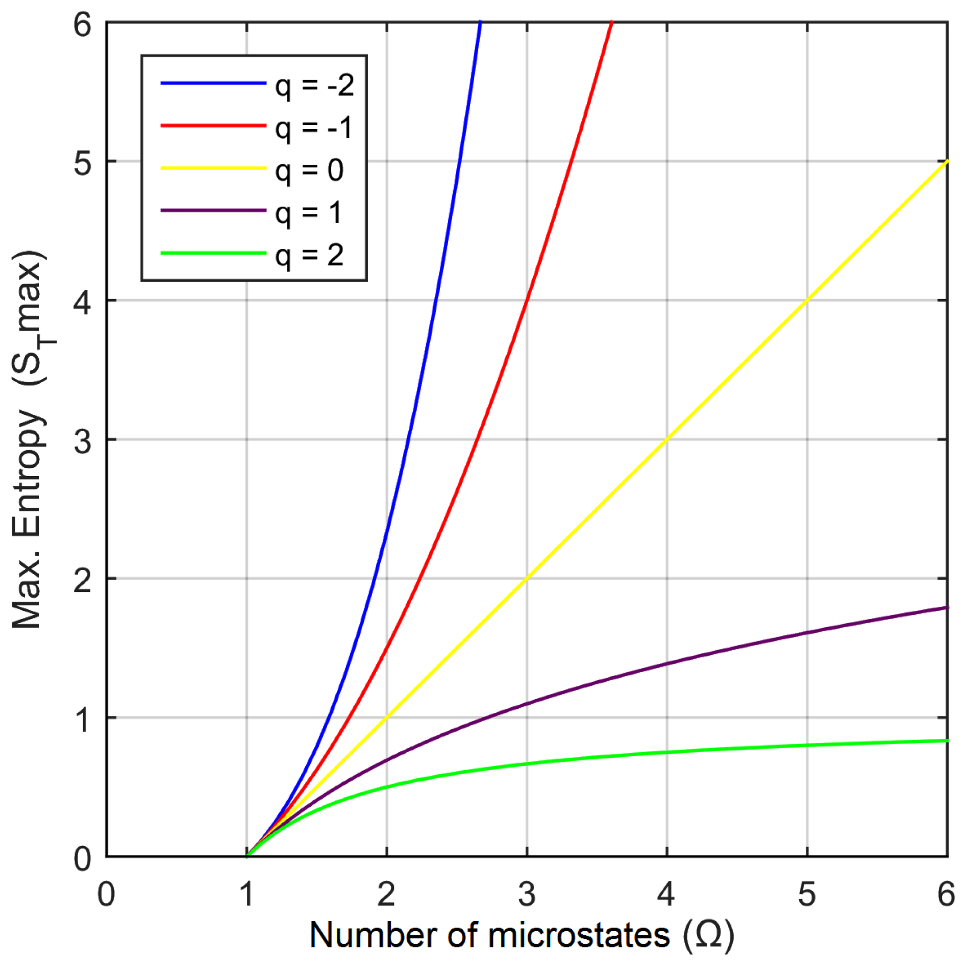
• $S_T$ has a maximum when each microstate is equiprobable, i.e., $p_i=1/\mathsf{\Omega },\forall i$, and it is given by:

  $$S_{T\max }=k\frac{1-{\mathsf{\Omega }}^{1-q}}{q-1}$$

  (6)

If $q>0$, then $S_{T\max }$ will be maximum; if $q<0$, then $S_{T\max }$ will be a minimum. If $q>1,S_{T\max }$ approaches $1/(q-1)$ when $\mathsf{\Omega }\to \infty$. If $q\le 1$, $S_{T\max }$, it diverges when $\mathsf{\Omega }\to \infty$. On the other hand, if $q\to \infty$, then $S_{T\max }\to 0$; it coincides with the x axis; but if $q\to -\infty$, then $S_{T\max }\to \infty$, i.e., it coincides with the y axis.

Figure 1 shows the $S_{T\max }$ as a function of number of microstates Ω, for several numeric entropic index values [10].

Tsallis entropy $S_T$ does not necessarily pretend to replace the successful Boltzmann–Gibbs entropy $S_{BG}$, but to face the problems where the classical statistical physics fails. The Tsallis entropy concept originates a completely new non-extensive statistical physics, which is really interesting and has many applications in theoretical and experimental physics. It is able to be applied to complex systems that are out of the Boltzmann–Gibbs statistics domain. As soon as Tsallis entropy appeared, a mathematical formalism was developed [19]. For example, q-exponential and q-logarithm functions were created:

$${\exp }_T\left(x\right)={\exp }_q\left(x\right)=\frac{x^{1-q}-1}{1-q}\mathrm{and}{\ln }_T\left(x\right)={\ln }_q\left(x\right)={\left[1+(1-q)x\right]}^{\frac{1}{1-q}}$$

(7)

These functions become the ordinal functions when $q\to 1$. In the notation used here, the sub-index of entropy is the first letter of the name of such entropy; some authors use q as a sub-index instead of T.

2.1. Shannon Entropy and Information Theory

The information theory is a mathematical theory that studies the transmission and the processing of the information; such a theory was consolidated by Claude E. Shannon in 1948 [17]. In this theory, the self-information or information is defined by:

$$I=-\log \left(p\right)$$

(8)

so, Shannon entropy $S_S$ is defined by:

$$S_S=-\sum _{i=1}^{\mathsf{\Omega }}{p}_i\log \left(p_i\right)$$

(9)

Last equation represents the mean information of a system. Here, Ω represents the system total number of events and $p_i$ the probability of the occurrence of each event, with $(1\le i\le \mathsf{\Omega })$ that satisfies Equation (3). The information theory is based on Shannon entropy $S_S$, which is Boltzmann–Gibbs entropy $S_{BG}$, but with $k=1$. The concept of redundancy represents a repetitive signal that does not generate new information, and it is defined by:

$$R_S=S_{S\max }-S_S$$

(10)

In information theory, the maximum entropy principle states that if inferences are to be made based on incomplete information, they should be drawn from the probability distribution that has maximum entropy permitted by the information that is already available [18,19,20,21,22]. This principle means that absolutely for any system, its entropy is bounded by a maximum entropy. From this point of view, the smaller the redundancy, the greater the information in the signal. This theory has a wide variety of technological repercussions, which have influenced all science an engineering areas, particularly for the area of image processing; see [3,4,13,16,23].

2.2. Tsallis Entropy and Information Theory

An alternative approach to information theory is the one that uses Tsallis entropy $S_T$ instead of Shannon entropy $S_S$ [3,13,19,22]. From this point of view, the information I, Equation (8), becomes q-information given by $I_T=-{\ln }_T\left(p_i\right)$, with ${\ln }_T\left(p_i\right)$ as in Equation (7); the redundancy R becomes q-redundancy given by $R_T=S_{T\max }-S_T$; and the maximum entropy $S_{S\max }$ becomes $S_{T\max }={\ln }_T\left(\mathsf{\Omega }\right)$ [5,13,16]. Under this approach, estimating the value of q becomes an important question. In the next section and for the goals of our research, we show a methodology to solve this problem.

3. Methodology to Calculate the Entropic Index q and Image Segmentation

The entropic index q is correlated with the complex internal interactions within the system. For digital images, we can also consider that the intensities of pixels have long-range correlations [24]. Originally, one of our goals was to segment images by using the entropy concept in a similar way to [3,5,16]. Here, it was important to know the entropic index, but usually it is estimated in an empirical way. Then, for the problem of our interest: when an image is given, what is the optimal value of its entropic index q? This, as far as we know, is not explicitly solved and reported in the literature, and instead, in image processing, usually most of the papers just use those values that give acceptable results often obtained by trial and error tests. Anyway, we do not agree to use a value for the entropic index q obtained in this “practical” way. That is why we started to search for a formal methodology to determine the entropic index q for a given image. We consider that each system has its own entropic index, and it must not be chosen “by eye”. Our research started by understanding physical systems already known. What we found was that there did not exist general procedures to solve the problem [10]. After that, we looked at information theory and did not find general procedures, but we focused our attention on two fundamental concepts: the redundancy concept and the maximum entropy principle.

Then, we looked for the entropic index q in an image by considering it as a non-extensive system. What we do is to consider images in grayscale in order to maximize their q-redundancy, that is:

$$R_T=1-\frac{S_T}{S_{T\max }}$$

(11)

From an information theory point of view, the smaller the redundancy, the greater the information in the signal. This is something very well known and allows one to calculate the entropic index q.

Then, we can calculate the redundancy $R_T$, as a function of the entropic index q, where q is evaluated from −∞ to ∞, since that q is a real number. The obtained graphic has an extreme value, which is associated with the optimal q, which is characteristic of the given image.

The procedure is applied as follows:

• Given an eight-bit grayscale image, we build its histogram, and then, we normalize it; the result is the probability distribution of the image, $p_i=\{p_1,p_2,\cdots ,p_{256}\}$. If $p_i=0$, remove it from the distribution, since such events give information $I=\infty$ and can be proven using L′Hôpital’s rule that the product $0·{\log }_{a}0=0·I_i=0$; that is why these cases are discarded.
• Once the probability distribution is known, the $S_T$ and $S_{T\max }$ are calculated using Equations (4) and (6). In this case, $\mathsf{\Omega }=256$, and a fixed q is used.
• Using the previous q, the redundancy $R_T$ is calculated through the Equation (11), then the ($R_T$, q) data of this type are obtained.
• Steps 2 and 3 are repeated with a different q to the one previously used, as many times as necessary, in order to get a reasonable curve ($R_T$ versus q). In our case, $q\in [-2,10]$ are considered, i.e., 1201 different values were considered for q.
• $R_T$ versus q is plotted, and the q value that maximizes the redundancy $R_T$ is identified. Such q will be q characteristic of the given image.

The previous procedure can work for any image represented as a pixel matrix or for any system in which we know a priori the probability distribution; that is, why we consider our procedure important.

Digital Image Processing Using Entropy: Segmentation

In general, image processing looks to give a better visual aspect or to make evident some information in the images through computing tools. The image processing procedure involves four areas: image formation, image visualization, image analysis, as well as image management. The analysis includes: feature extraction, segmentation, classification and enhancement [1]. Our main interest is image segmentation, which has many and important applications. Image segmentation means to divide into regions with common characteristics; for example, to separate the image into two regions as the background and the object. Segmentation is a stage that generally precedes classification [1], as mentioned before.

Furthermore, as mentioned above, image segmentation using thresholding based on its histogram is one of the most common approaches due to its easy implementation and requires less computing resources to run. There are two thresholding methods: the first is called global if a single threshold is calculated for the entire image; the second is called local or adaptive if the image is divided into regions and a threshold is calculated for each region [2].

The major disadvantage of the histogram-based thresholding methods is their disregard of the spatial context within which the intensity value occurs. In other words, they do not consider the intensity values of the surrounding pixels. Methods based on 2D histograms consider, up to some degree, contextual information. Thresholding methods are also frequently used for the initial segmentation of images prior to the application of a more sophisticated segmentation method for the purpose of reducing the convergence time [1,2].

4. Image Thresholding Using Tsallis Entropy

A method of segmentation is carried out by thresholding. There are several procedures to thresholding an image, such as the ones shown in [1]. The most intuitive approach is the global thresholding, where only one gray threshold level is selected from the histogram [25]. The threshold separates the histogram into two sets; gray levels less than or equal to the threshold will be zero, and the gray levels greater than the threshold will be one. The thresholding transforms the original image (in grayscale) into a binary image (black and white). There are several ways to find the optimal threshold in an image. We consider procedures based on Tsallis entropy and the Shannon entropy as [2,3,4]. This methodology is not the same one that was used to calculate the index q.

Below, we will show how to use the Tsallis entropy for image thresholding. Let the image be considered as a pixel matrix of size $m\times n$ with $x\in 1,2,\cdots ,m$ and $y\in 1,2,\cdots ,n$ of eight bits in grayscale. Let $f(x,y)$ be the gray level in the $(x,y)$ pixel of the image. Let $h\left(a\right)$ be the image histogram with $a\in \{0,1,2,\cdots ,255\}=D$.

From the $h\left(a\right)$ histogram, the probability distribution $\left\{p_i\right\}=\{p_1,p_2,\cdots ,p_k\}$ can be calculated, where ${\sum }_{i=1}^k{p}_i=1$ (k represents the gray levels).

At this point, our goal is to calculate an optimal threshold $t^{*}$ (with $t^{*}\in D$), which divides the histogram $h\left(a\right)$ in such a way that it separates the two most representative objects of the image, for example the background and the object. This optimal threshold $t^{*}$ is calculated considering the image as a non-extensive system, i.e., with the Tsallis entropy. Of the distribution $\left\{p_i\right\}$, two probability sub-distributions are built: the one from object A and the one from the background B as follows:

$$P_A=\sum _{i=1}^t{p}_i,P_B=\sum _{i=t+1}^k{p}_i$$

(12)

where conditions $0\le P_A\le 1$ and $0\le P_B\le 1$ must be held, so that both distributions must be normalized:

$$P_A:\left\{\frac{p_1}{P_A},\frac{p_2}{P_A},\cdots ,\frac{p_t}{P_A}\right\},P_B:\left\{\frac{p_{t+1}}{P_B},\frac{p_{t+2}}{P_B},\cdots ,\frac{p_k}{P_B}\right\}$$

(13)

with $p_A+p_B=1$. Next, the Tsallis entropy is calculated for each set A and B:

$$S_T^A\left(t\right)=\frac{1}{q-1}\left(1-\sum _{i=1}^t{p}_i^q\right),S_T^B\left(t\right)=\frac{1}{q-1}\left(1-\sum _{i=t+1}^k{p}_i^q\right)$$

(14)

The Tsallis entropy $S_T$ is parametrically dependent over the threshold value t to the object and background. The pseudo-additivity property is applied to the sub-sets A and B, which are supposed to be statistically independent, that is:

$$S_T^{A+B}\left(t\right)=S_T^A\left(t\right)+S_T^B\left(t\right)+(1-q)S_T^A\left(t\right)S_T^B\left(t\right)$$

(15)

The next step is to maximize the quantity of information $S_T^{A+B}\left(t\right)$ between the two sub-distributions previously created in order to obtain the maximum information between the two created regions. This works because the maximum of possible information is transferred when the total entropy of both systems is maximum [23]. Then, we must consider the t that maximizes $S_T^{A+B}\left(t\right)$; such a t will just be the $t^{*}$ that is given by:

$$t^{*}\left(q\right)=\underset{t\in G}{\text{arg max}}\left[S_T^A\left(t\right)+S_T^B\left(t\right)+(1-q)S_T^A\left(t\right)S_T^B\left(t\right)\right]$$

(16)

Notice that t depends on the entropic index q, which is estimated empirically in many papers [5,16,24]. Nevertheless, we use the q calculated through the previously-described method, and it characterizes the image.

Remember that the Tsallis entropy (Shannon entropy generalization) includes the extensivity and non-extensivity of a system, so that it is reasonable to think that Tsallis entropy is better than Shannon entropy.

Once the threshold $t^{*}$ is obtained, the next step is to create a binary thresholding image $g(x,y)$. This image is created with the following criteria: $g(x,y)=0$ if $f(x,y)\le t^{*}$, and in the opposite case, $g(x,y)=1$.

4.1. Image Thresholding Using Shannon Entropy

When $q\to 1$ in Tsallis entropy, Shannon entropy is obtained, so that the method considers now the following expression, according to [16]:

$$t^{*}\left(q\right)=\underset{t\in G}{\text{arg max}}\left[S_T^A\left(t\right)+S_T^B\left(t\right)\right]$$

(17)

This expression is the function that allows one to find $t^{*}$.

4.2. Image Binarization and Edge Detection

In this part of the work, images are segmented by using Tsallis entropy and Shannon entropy, in order to compare both of them. The purpose is to show the advantages when using the Tsallis entropy. These procedures are already known, but the main point here is to show the benefit of knowing a priori the entropic index q of an image, according to the method in [3]. The binarized image is generated using the optimal threshold $t^{*}$ obtained by Tsallis or Shannon entropy.

Generally after segmentation, a detection of edges procedure is applied. Even though there are sophisticated methods to detect edges, we simply apply a Sobel filter to the segmented images.

All of these procedures mentioned above were implemented in the software MATLAB^® R2015a and are summarized in the algorithms, described in the Supplementary Materials.

5. Results and Discussion

As was mentioned before, from the information theory point of view, which uses $S_S$, the smaller the redundancy, the greater the information in the signal. The previous claim is something well known in information theory; nevertheless, what we did was to generalize this claim, but in Tsallis entropy terms. Here, the redundancy R becomes q-redundancy $R_T$; this allows us to find the q, which represents a given system through the maximum redundancy. Then, q associated with this maximum will be the one that represents the given image, knowing that any image has a maximum entropy, that is when each microstate is equiprobable. Then, from the above, it is possible to construct a general method, which can be applied whenever the probability distribution of the system is known. Additionally, it is trivial to know the probability distribution of an image based on its histogram.

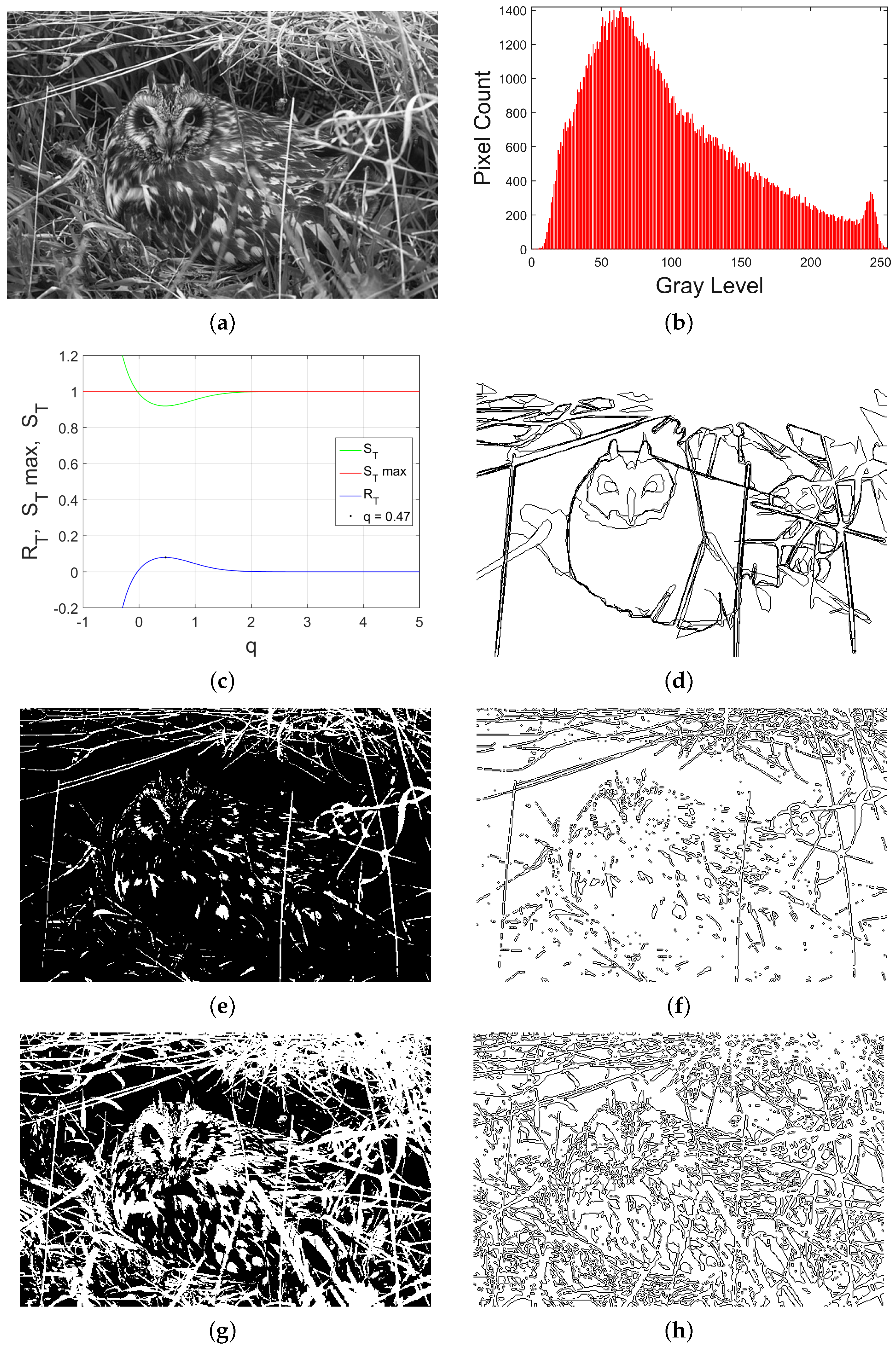
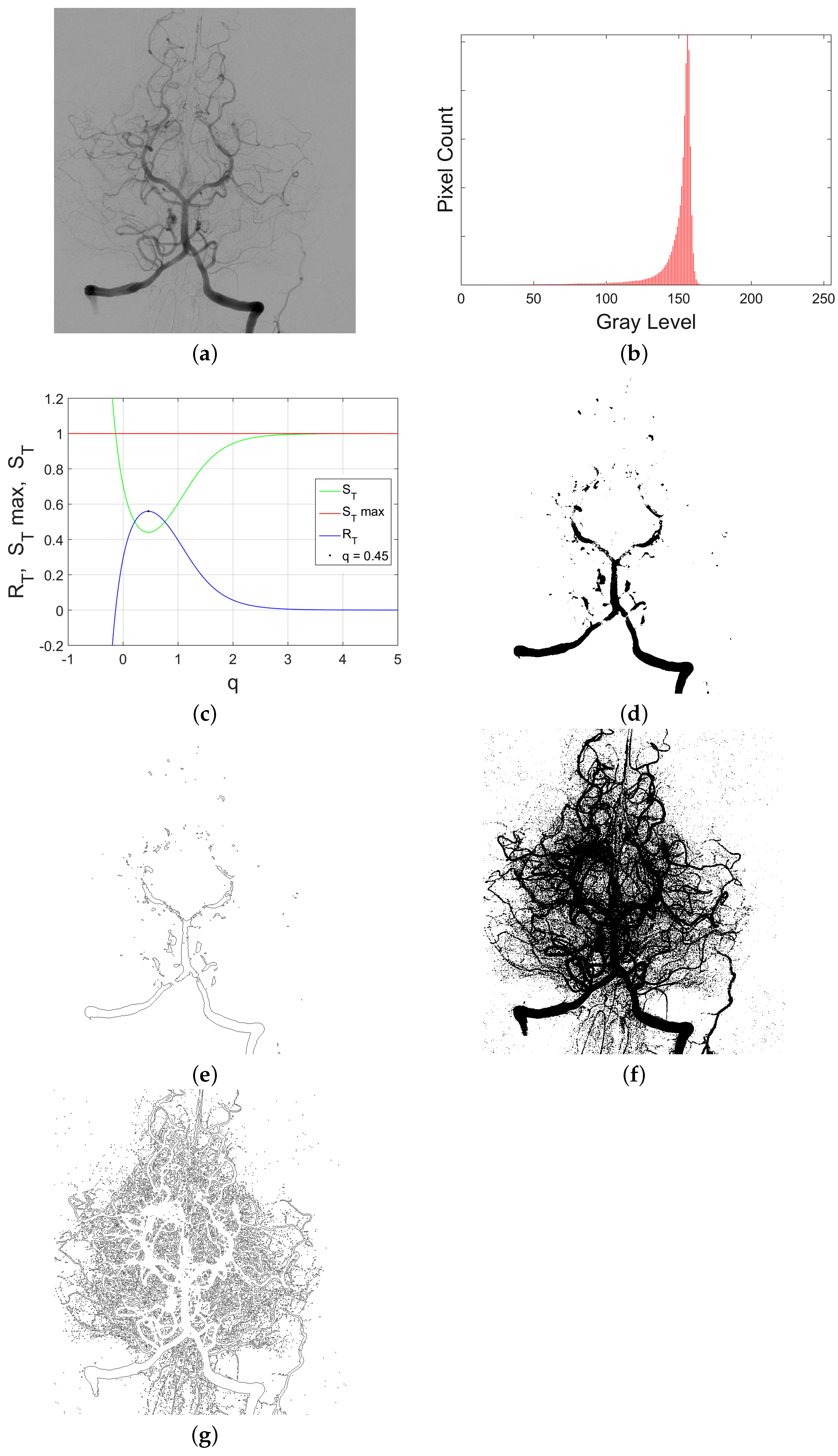
We choose three typical images used in image processing (“Lena”, “Owl” and “Moon”), obtained from [26,27,28,29], as well as a cerebral “Angiography” obtained from [30]; cerebral angiography helps determine the extent of vascular problems within cerebral blood vessels, Figure 5 showing a transverse projection of the vertebrobasilar and posterior cerebral circulation. Next, we calculated the $S_S,S_T$ and q for the “Lena”, “Owl”, “Moon” and “Angiography” images. The index q became a number between zero and one, i.e., they are sub-extensive systems ($q\ge 1$). It was useful to normalize the $S_T$ and $R_T$, where $S_T \max =S_T+R_T$, so that $S_{T\max }$ represents $100\%$ of the total entropy possible. 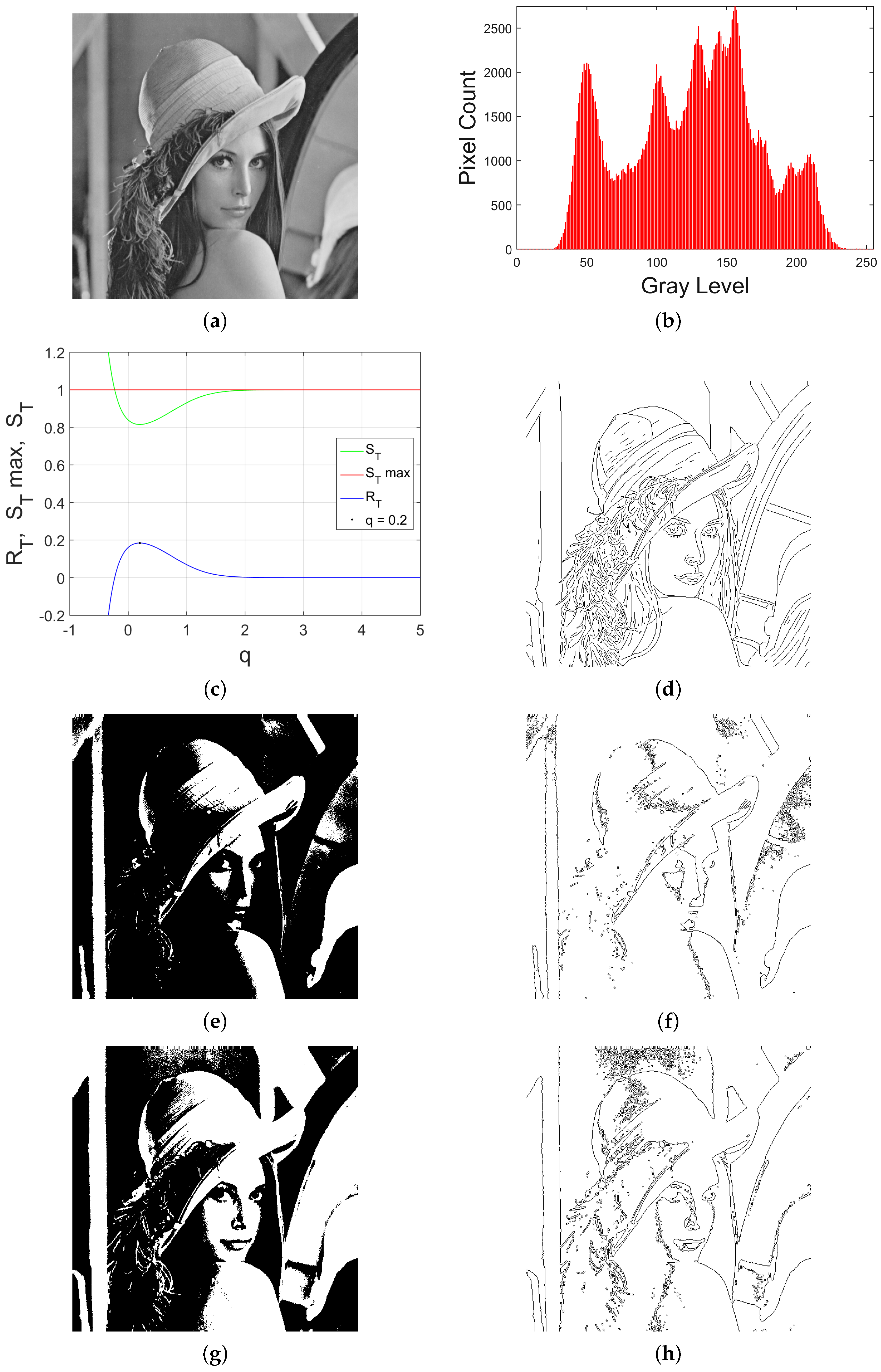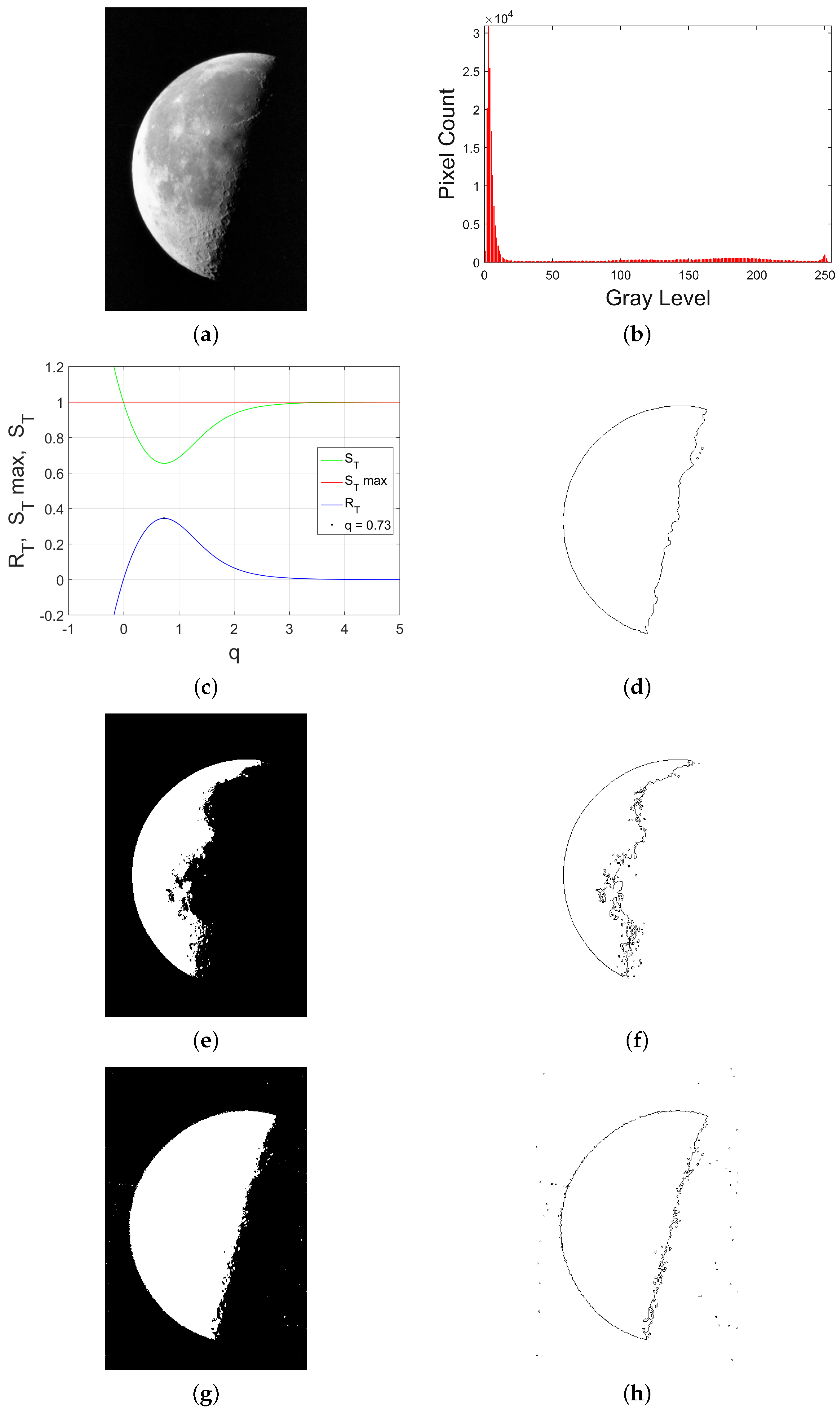The studied images, as well as the index q calculated, are shown in Figure 2, Figure 3, Figure 4 and Figure 5.

The “Moon” image was the one with the most redundancy (36%), which makes sense due to the fact that it is the image that has the most similar pixels, according to its histogram. The opposite case happens to the “Owl” image, which has a minimal redundancy (8 %), which makes sense due to the fact that it has a great variety of colors, almost all of the grayscale, as shown in the original image and its histogram. The “Lena” image has a redundancy of almost 20%, and the “Angiography” image has 51%.

The entropic index values q computed are shown in

Table 1. Numerical results using Shannon and Tsallis entropy with the index q calculated.

Image	Shannon	Optimal	Tsallis	Entropic	Redundancy	Maximum	Optimal
	Entropy $S_S$	Threshold	Entropy $S_T$	Index q	$R_T$	Entropy $S_{T\max }$	Threshold
Lena	5.16 nats	160	85.04 nats	0.20	19.27 nats	104.31 nats	132
Owl	3.82 nats	172	31.07 nats	0.47	2.69 nats	33.76 nats	89
Moon	5.29 nats	159	8.42 nats	0.73	4.42 nats	12.84 nats	17
Angiography	3.35 nats	105	15.14 nats	0.45	19.99 nats	35.13 nats	151

. All of the procedures were made in Shannon entropy terms in order to compare them.

Segmented Image and Edge Detector Using Tsallis and Shannon Entropy

In order to test the calculated index q, we segmented images by Tsallis and Shannon entropy. The optimal thresholds obtained by Shannon entropy and Tsallis entropy are also shown in Table 1. The images segmented by Shannon entropy and Tsallis entropy (include our index q) are shown in (e) and (g), in Figure 2, Figure 3 and Figure 4. In Figure 5, these are shown in (d) and (f).

The final step is to apply a Sobel filter to the segmented images in order to detect edges. The best results were obtained when the Tsallis entropy was used. The results are shown in (f) and (h), in Figure 2, Figure 3 and Figure 4. In Figure 5, is shown in (e) and (g).

For the purpose of evaluating the procedure, we can do a qualitative comparison from our results with the ground-truth edge image (see (d) in Figure 2, Figure 3 and Figure 4). Ground-truth “Owl” is available in the dataset [27]. Ground-truth “Lena” and “Moon” were made by a human expert. Ground-truth “Angiography” is not available. Quantitative and qualitative methods of evaluation can be found in [31].

All of the procedures mentioned can be generalized relatively easily to color images (RGB), where each color corresponds to a grayscale level. This is a procedure on which we will be working later. Such procedures are very important in the artificial vision, as well as in imaging, even though we only consider now optical images.

All of the procedures can be applied multiple times to the images in order to obtain the sub-threshold using recursivity, which allow more advanced segmentations.

Another important point that remains for a future work is that it is possible to characterize image regions through local entropic indices. For example, thinking of a medical image, we could be able to characterize different tissues by their corresponding entropic indices q.

6. Conclusions

Calculating the entropic index q is in general an open topic; q can only be determined in very particular problems. Considering q-information, q-redundancy and the probability of the distribution in an image, as well as applying the maximum entropy principle, we propose a method to computing the entropic index q, where the images are considered as non-extensive systems. This is a numerical procedure that consists of finding the maximum in the curve given microstates vs. q-redundancy. This procedure can be applied not only to images, but also to any system only if the probability distribution is known.

In order to prove the advantages of knowing the entropic index q, a thresholding image procedure was implemented. It was also used in the Tsallis entropy, finding better results when q is known. This is better than when Shannon entropy is used. Similarly, edge detection procedures are better when Tsallis entropy is used with a known q. Our proposal is applied to any kind of images, with a great variety of applications in computer vision or imaging.