Article

Fast EEMD Based AM-Correntropy Matrix and Its Application on Roller Bearing Fault Diagnosis

1
State Key Laboratory of Rail Traffic Control and Safety, Beijing Jiaotong University, Beijing 100044, China
2
School of Electric Engineering, Beijing Jiaotong University, Beijing 100044, China
3
Beijing Research Center of Urban Traffic Information Sensing and Service Technologies, Beijing Jiaotong University, Beijing 100044, China
4
School of Electrical Engineering and Automation, Jiangxi University of Science and Technology, Ganzhou 341000, China
5
School of Business, University of Wollongong Australia, Wollongong 2519, Australia
*
Author to whom correspondence should be addressed.
Entropy 2016, 18(7), 242; https://doi.org/10.3390/e18070242
Submission received: 2 May 2016 / Revised: 18 June 2016 / Accepted: 21 June 2016 / Published: 28 June 2016
(This article belongs to the Section Complexity)

Abstract

:
Roller bearing plays a significant role in industrial sectors. To improve the ability of roller bearing fault diagnosis under multi-rotating situation, this paper proposes a novel roller bearing fault characteristic: the Amplitude Modulation (AM) based correntropy extracted from the Intrinsic Mode Functions (IMFs), which are decomposed by Fast Ensemble Empirical mode decomposition (FEEMD) and employ Least Square Support Vector Machine (LSSVM) to implement intelligent fault identification. Firstly, the roller bearing vibration acceleration signal is decomposed by FEEMD to extract IMFs. Secondly, IMF correntropy matrix (IMFCM) as the fault feature matrix is calculated from the AM-correntropy model of the primary vibration signal and IMFs. Furthermore, depending on LSSVM, the fault identification results of the roller bearing are obtained. Through the bearing identification experiments in stationary rotating conditions, it was verified that IMFCM generates more stable and higher diagnosis accuracy than conventional fault features such as energy moment, fuzzy entropy, and spectral kurtosis. Additionally, it proves that IMFCM has more diagnosis robustness than conventional fault features under cross-mixed roller bearing operating conditions. The diagnosis accuracy was more than 84% for the cross-mixed operating condition, which is much higher than the traditional features. In conclusion, it was proven that FEEMD-IMFCM-LSSVM is a reliable technology for roller bearing fault diagnosis under the constant or multi-positioned operating conditions, and as such, it possesses potential prospects for a broad application of uses.

Graphical Abstract

1. Introduction

As one of the pivotal mechanized devices, roller bearings constantly rotate in harsh industrial environments that often feature high temperatures, variable rotational speeds, and big loads; as such, they have a high breakdown probability [1]. It is difficult to diagnose roller bearing faults because the fault burst of the roller is strong and because the ambient noise and hectic operating conditions in which they generally exist; as a result, the condition of the roller bearings may represent hidden dangers for mechanical and electrical systems. Consequently, it is of great significance to develop identification techniques for determining the condition of roller bearings in order to ensure the safety of the facility and its operations. For this reason, the fault diagnosis of roller bearings has been a research focus in various related fields.
Currently, pattern recognition is one of the popular roller bearing fault diagnosis approaches which has constantly been developing from its initial form of distinguishing the condition of roller bearings by analyzing sound differences. At present, many approaches have been proposed to achieve successful roller bearing fault diagnosis [2,3,4]. The current fault diagnosis technical structure includes two aspects: feature extraction and pattern identification [5]. A good pattern identification method is admittedly important, but there is no norm to follow in order to ascertain the best pattern identification parameters. Moreover, in order to fundamentally improve the fault diagnosis ability, it is more convincing to determine a fault divisible feature, which can be revealed in a variety of forms in order to show the diagnosis results.
Before extracting the fault features of roller bearings, the state parameter should first be extracted. Some fault features can be expressed in state parameters, such as the axial temperature and rotor current. However, these state parameters are similar in that they can only diagnosis the late and serious faults. In order to find the early faults of the bearings in order to keep the devices safe, some roller bearing state parameters such as vibration acceleration and ultrasonic waves have been used [6]. In considering that the ultrasonic wave is easy to be interfered by noise, this welcomed extracting technique currently refers mainly to the measurement of vibration by suitable transducers [7]. However, it is difficult to extract characteristic information directly from the vibration signal of roller bearings which are non-stationary, non-linear, and which often feature strong noise interference [8]. The general way to extract fault features is based on adaptive time frequency transformations. Empirical Mode Decomposition (EMD), proposed by Huang [9], is a typical adaptive time-frequency decomposed method which is affected with the mode mixing problem [10]. To solve the problem, Huang has put forward the detection interrupted method [11], which is a kind of posteriori judgment that has many limitations. Ensemble Empirical Mode Decomposition (EEMD) is another method to eliminate the mode mixing problem which has been proposed by Wu in 2009 [12]. This approach adds white noise data onto the primary signal, applying the uniform distribution character of the white noise frequency spectrum to make up for the absence of the signal scales. Meanwhile, the characteristic zero-mean statistic of white noise is employed in order to remove the added noise influence, so that the decomposed result can be better than the single EMD algorithm. However, many groups of white noise and many EMD processes increase the computation complexity of EEMD. Furthermore, the real-time calculation of EEMD may be influenced if the program structure is confused. To improve the computation efficiency of EEMD, many researchers have tried various approaches [13,14]. Among all the studies, Wang [15] has analyzed the computing intensity of EMD and EEMD and verified that the computational complexity depends on the data length. Based on the computational evidence he has concluded that the EEMD time cost can be shortened as Fast EEMD (FEEMD). The improved effect of FEEMD has been applied on wind speed forecasting [16]. In terms of Intrinsic Mode Function (IMF) features, although the combination of EEMD and information theory has been a hot research topic in recent years [17,18], it pays little attention to the attempt of considering cross correlation information as fault features. Among the cross correlation measures, Correlation Function (CF) as a time structure similarity measure has been widely applied in signal processes such as statistical analyses [19,20] , trait associations [21], and so on. However, CF is limited to reflect two order moment statistical traits between two signals only, and furthermore, its ability to analyze non-Gaussian and nonlinear signals cannot avoid severe attenuation [22]. Correntropy, which was advanced by Santamartía in 2006 [23], is a generalized correlation measure which contains even order moment statistical information. More detailed correlative information demonstrates that correntropy is more sensitive and the implementation of the kernel function can be more appropriate means in which to deal with high dimensional nonlinear signals than CF [24]. Because of these properties, in recent years, correntropy has been further studied in different subject fields, such as time series modeling [23], nonlinearity testing [24], feature selection criterion [25], hyper spectral immixing [26], gross error detection [27], medical signal processing [28], and so on. To achieve state identification, the Support Vector Machine (SVM) method has been widely employed in the machine learning community because of its distinctive generalization ability compared with that of other conventional methods, such as the neural network method [29]. Built on the foundation of the SVM algorithm, the Least Square Support Vector Machine (LSSVM) method possesses not only as good of a generalization ability as the general SVM method, but a better learning ability for small samples than the general SVM method. In addition, the calculation speed of LSSVM is faster than SVM based on the same identification accuracy [30] That is why LSSVM is prevalent in many fields related to pattern recognition [31,32].
Therefore, in terms of bearing fault feature extraction, the correlative information between time-frequency components and primary signals can be potential cachets. To extract the cachets comprehensively, here we propose the IMF correntropy matrix (IMFCM) which is comprised of four dimensions which are: fault state class, total number of sample data, data length, and IMF number in each FEEMD process. The centralized computation of a fault feature set can reflect the unity and logic of the sample set. The consequences of roller bearing fault identification will be obtained through LSSVM. In short, the purpose is to verify the performance of FEEMD and the divisibility and robustness of IMFCM in roller bearing fault diagnosis are better than the existing methods.
This paper contains seven sections. The first part introduces the basis of the study. The second section presents the research framework. The third part considers the instruction of the algorithms used to extract the fault features, and contains two subsections: the fast empirical mode decomposition algorithm and the definition and computation scheme of IMF correntropy matrix. The fourth sections discusses the application of IMFCM in fault identification, and contains two sub-sections: a brief overview of the Least Squares Support Vector Machine method and an evaluation of the identification consequence. The fifth section contains a case study and applicability experiment that considers both a Stationary Operating Situation and Cross-mixed Operating Situation. The sixth section is a discussion that analyzes the results of the experiment. The last part is the conclusion which summarizes the whole research work.

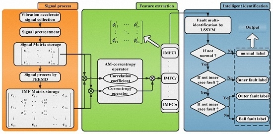
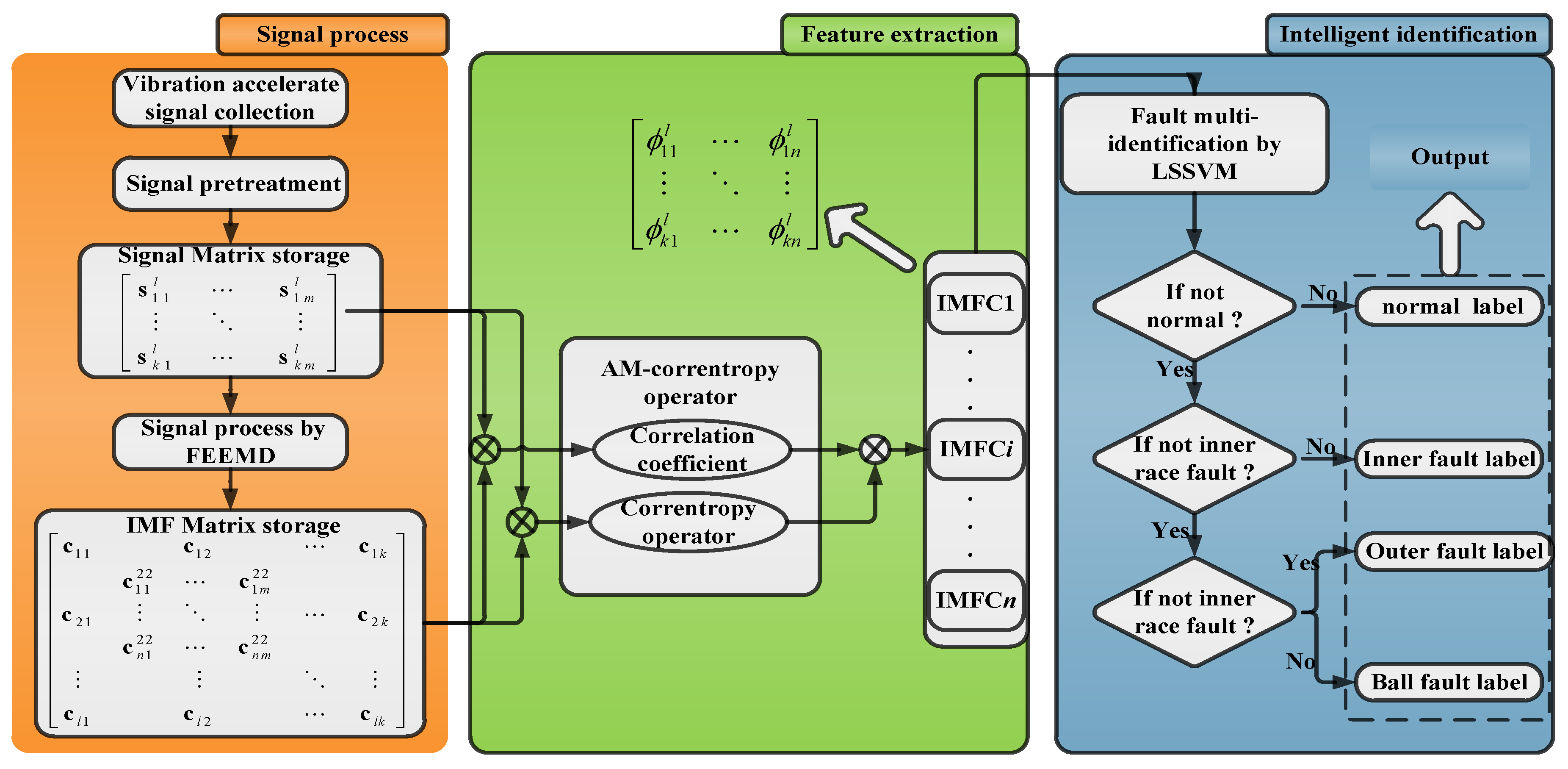
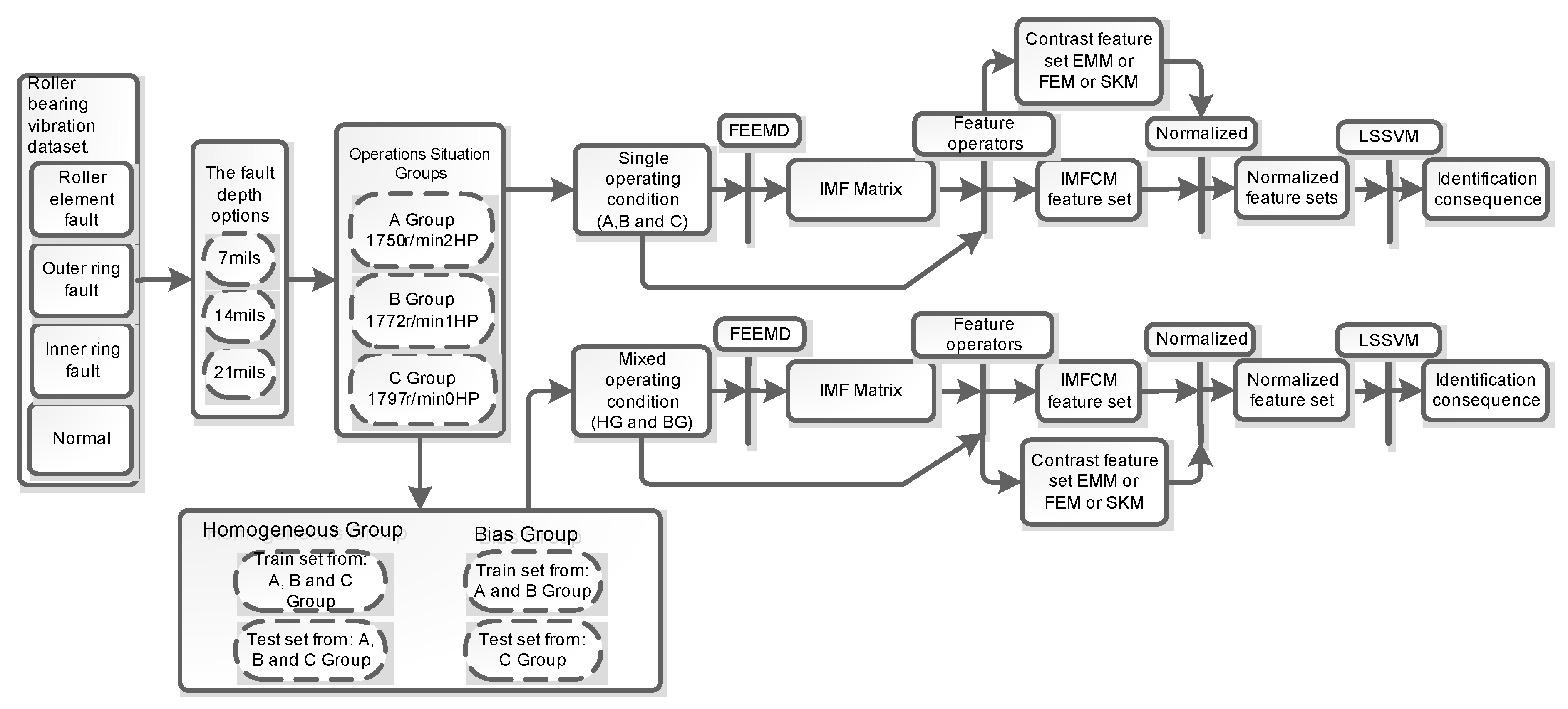
2. The Method Framework

The method framework contains three sub-procedures: the signal process, the feature extraction, and the state identification. The signal process is composed of a series of processes. In particular, the vibration acceleration signal is collected regardless of the operating condition of the roller bearings. The detailed framework for implementing the roller bearing fault diagnosis is shown in Figure 1. The parameters of s, c, and ϕ are for the primary vibration signal of roller bearings, the IMF decomposed from the primary signal, and the AM-correntropy, respectively. k, l, m, and n refer to the number of fault style, the number of primary signal samples, the length of each sample, and the amount of IMFs decomposed by a primary sample. The detailed mathematical relationships of the above parameters will be described in the following sections.

3. Instruction of Algorithms to Extract Fault Feature

3.1. Fast Empirical Mode Decomposition Algorithm

3.1.1. Brief Overview of EMD and EEMD Algorithms

To realize the stationary signal processing, the EMD algorithm separates the wave motion or tendency into different scales step by step, and then IMFs, a series of signal sequences with different characteristic scales, will be obtainable. To be an IMF, a sequence should follow two conditions:
  • The number of extreme value points and the number of zero-crossings must either be equal or differ at most by one in the whole primary signal.
  • At any point, the mean value of the envelope defined by local maxima and the envelope defined by the local minima is zero. The upper and lower envelopes are of local symmetry about the timeline.
The IMFs disassembled by EMD that satisfy the above two criterions are all near single frequency components and almost orthogonal signals [9]. The detailed description of the EMD algorithm execution process can be referenced in [9].
To prevent a primary single component signal from losing its physical meaning in the IMF sifting process, the stop norm is added to stop the sifting process. The general stoppage criterion makes use of standard deviation (SD) [16] as the stop condition. Besides the SD, there are many other stoppage criteria in applications such as the three parameters rule [33] and energy difference tracking method [34].
However, a susceptibility to mode mixing is one of the EMD shortcomings, which may reveal the signal’s characteristic information incorrectly and may generate the crucial influence of the specific physical background [35].
To assuage the drawback of mode mixing which is intrinsic in the performance of EMD, EEMD was proposed by Wu and Huang [12]. To eliminate the intermittency of the primary signal, and then restrain the generation of mode mixing effectively, it is necessary to add white Gaussian noise with different amplitudes before each decomposed step, as white Gaussian noise has the statistical property of uniform distribution in the whole time-frequency domain, making the signal continuity better and more easily eliminated by superposition. Meanwhile, the statistical mean value of unrelated random noise has been proved to be zero, so the ensemble mean calculation of the IMFs can almost remove the interference of white noises. The procedure of EEMD can be depicted as follows [12]:
Add numerically generated white noise δi(t) on the primary signal s(t) as demonstrated in the following equation, where i means the i-th trail of adding white noise with ne trails, and i = 1, 2, …, ne:
s i ( t ) = s ( t ) + δ i ( t )
Decompose the signal si(t) by EMD algorithm to get several IMFs cij(t) and a residue ri(t), in which cij(t) is the j-th IMF component of the i-th EMD of si (t) with j = 1, 2, …, n, and ri(t) is the i-th EMD residue.
Step One: Repeat the two aforementioned steps, and add different white noise sequences with the same root mean square each time.
Step Two: Calculate the ensemble means cj(t) of the corresponding IMFs of the decompositions as the final IMFs which can be represented by the following equation:
{ c j ( t ) = 1 n e i = 1 n e c i j ( t ) r ( t ) = 1 n e i = 1 n e r i ( t )
where cj(t) is the j-th IMF component decomposed from the primary signal using EEMD.

3.1.2. Brief Overview of Fast EEMD

It is obvious that the process of EEMD indicates a more sophisticated signal processing technique for nonlinear and non-stationary signals than EMD. Hence, EEMD generates more computational complexity [14].
Practically, Wang [15] has proven that the computing process of EMD and EEMD is not intensive and tedious. It has been demonstrated that the computational time complexity (CTC) of EMD is no greater than ns·(41·n·m), which is proportional to shifting time ns, IMF dimension n, and signal length m, and the CTC of EEMD is no greater than NE·ns·(41·n·m), which is proportional to the EMD CTC and ensemble time ne respectively. Generally, getting ne by SD stoppage criterion costs at least 5m CTC. The fast EEMD (FEEMD) algorithm indicates that the fixed value of ns can perform better than the ns obtained by other stoppage criteria. Furthermore, it has been summarized by Wu [12,36] that to get better decomposed results the assignment of ns should generally be 10. Taking ns and ne as constants, the CTC of FEEMD can be described as T(m) = O(logm) [15], where n = log2m for EMD is performed as a dyadic filter bank [36]. Nevertheless, using the SD criterion the CTC of EEMD is no less than 205·ne·m2·log2m = O(m2·logm). The theoretical curve of the relationship between log10(CTC) and data length m is shown in Figure 2.

3.2. Definition and Computation Scheme of IMF Correntropy Matrix

The length of primary signal s(t) is m and the sample amount of primary signal is l, to construct primary signal matrix s(t)l × m under k-th fault states separately, it generates the sample matrix (SM) of k × l × m dimensions. Next, after the FEEMD process of each signal si(t), n IMFs are totally generated, then all the IMFs should be blocked in k × l × n × m IMF matrix (IMFM) to be processed more efficiently by the computer.

3.2.1. Brief Overview of Correntropy

For determining more reliable fault features, it is worth clarifying the proportion of each IMF component in the primary signal and the distance of every sampling point in each IMF component that leaves from the corresponding point in the primary signal. In considering this situation, the minutia is similarly significant and needs to be examined.
Correntropy is a generalized similarity measure that estimates the probabilistic similarity between two arbitrary random variables [37]. It is computationally intensive to determine the correntropy of two-dimensional random variable in a high-dimensional data space. The kernel function aims to solve the high-dimension problem of computation without specification of the nonlinear transformation function. Through the kernel function, the obtainment of the linear correlation information can be implemented in the higher dimensional linear space, which is the projection of lower dimensional nonlinear space. Correntropy as a continuous function has been deeply analyzed in the literature [23,24], however the computer can only handle the data discretely. Suppose that X and Y are two discrete random variables with m sampling points. Generally, the joint probability function PXY of X and Y is unknown and the sampling point amount m is a finite integer, thus the correntropy is calculated by the discrete sample estimation instead of the continuous correntropy model. The equation is as follows.
V ^ ( X , Y ) = E X Y = 1 m i = 1 m K ( x i , y i )
where K is the arbitrary positive definite kernel function which satisfies Mercer’s Conditions [24]. The Gaussian kernel (also called the radial basis function (RBF) kernel) is employed here to calculate the correntropy. The sample estimation of correntropy with the Gaussian kernel function is described as follows:
V ^ σ ( X , Y ) = 1 m 2 π σ i = 1 m exp ( x i y i 2 σ )
The size of the kernel scale parameter σ determines the metric of similarity in the reproducing kernel Hilbert space (RKHS). Experientially, the kernel scale parameter σ is generated by the Silverman standard [24]. However, to keep the fixed inner product in RKHS, it needs a fixed σ value which is determined to be 0.5 for a balanced effect here. Additionally, it is necessary to keep the same computation for each feature value in order to ensure the fault diagnosis results are meaningful. It can be observed in Equation (4) that correntropy obeys two rules: symmetry (V(X,Y) = V(Y,X)) and boundedness (0 < V(X,Y) < 1/ 2 π σ ). The correlation information can be revealed by Taylor’s series expansion of correntropy, which is shown in Equation (5):
V σ ( X , Y ) = 1 2 π σ m = 0 ( 1 ) m 2 m m ! E X Y [ ( x y σ 2 m ) 2 m ]
It contains a two order term of self-correlation information while m = 1 and an independent component analysis correlated term while m = 4. The weighted sum of even order moments reflects that correntropy includes all even order statistic messages, where a two order term makes up the major component and the quick attenuation of high order terms follows the addition of σ. Correntropy is therefore two order statistics with more ascendancy thereby implying more correlation statistical information, less information redundancy, and better correlation robustness than traditional correlation approaches.

3.2.2. Derivation of IMF Correntropy Matrix

Being that it is based upon the accumulation of local similarity, correntropy is considered as a local similarity measurement so that the linear degree of signal is negligible. In addition, each IMF component in the time domain has independent data distributions with partial similarity with the primary signal. As such, correntropy can measure the local similarity between IMF and the primary signal. Hence, it is sensitive to the local shock response. However, linear similarity is another measurement which contains the global similarity information that correntropy lacks. Adding the linear correlation coefficient as an AM operator, results in improved correntropy will which is called IMF-original-signal correntropy (IMFC). Based on the IMFC feature, the different fault styles of roller bearings can be embodied. Supposing ρ is the correlation coefficient between the primary signal and the IMF component.
ϕ = ρ 2 m σ { i = 1 m exp ( c i s i 2 σ ) }
where ϕ = V ^ (PF,S). The above part has mentioned that IMFM is k × l × n × m dimensional, thus one signal’s IMFC estimate ϕ is of 1 × n dimensions. Using Φ = (2)−1∙∑exp(−∥H∥⋅(2σ2)−1) as the correntropy operator, where ∥·∥ is the Euclidean norm and H = c n × m s 1 × m is the input matrix, then the IMFC vector ϕ 1 × n can be solved as follows.
ϕ 1 × n = Φ ( c n × m s 1 × m )
In order to reduce the calculation sophistication, it takes the followed equation to normalize ϕ so that the normalized solution ϕ can be obtained.
ϕ 1 × n = ϕ 1 × n i = 1 n ϕ i
To extend Equations (7) and (8) to all the primary signal samples in the whole state set, assuming Δ = k × l, Ω = Δ × n, then the calculation process of the Ω-dimensional IMFC matrix (IMFCM) is described as follows:
ϕ Ω = Φ H n m = Φ [ c 11 Δ s 1 Δ c 1 m Δ s m Δ c n 1 Δ s 1 Δ c n m Δ s m Δ ] = [ ϕ 11 k ϕ 1 n k ϕ l 1 k ϕ l n k ]
where c and s signify the sample matrix of ckl and skl, and ϕ Ω is the initial IMFCM. Furthermore, to express the convenience of calculation, it is necessary to partly transpose ϕ Ω . Accordingly, drawing support of Γ = (k × l)′ × n, ϕ Γ is the final target result of IMFCM.

4. Application of IMFCM in Fault Identification

To implement the fault identification based on IMFCM, the intelligent decision-making algorithm should be involved in this work. There are many studies of roller bearing fault identification that draw support from SVM [38]. As the development of SVM, LSSVM has been widely used recently for its faster calculation ability than SVM. Besides, it is of the same significance to choose an exhaustive index to evaluate the identification consequence. Here, LSSVM and its output evaluation are briefly analyzed accordingly.

4.1. Brief Overview on Least Square Support Vector Machine

Based on the structural risk minimization principle, the Support Vector Machine (SVM) method as one of the machine learning approaches can perform well in the analysis of a small capacity, high dimensional, and non-stationary sample set. The core idea of SVM is to build up a hyperplane as a decision surface in order to maximize the isolated edge of sample sets of different types. The linear discriminant function is used to divide the object samples into two classes. Supposing ω is the weight vector and x ϵ R[m,n] owns n samples, each of which has m dimensions.
y = sgn ( ( ω x ) + b )
However, nonlinear classification discrimination needs the nonlinear function ϕ(x) to map samples to high-dimensional linear space, and then the optimal classification hyperplane is constructed in the high-dimension linear space. Training sample number affects computation speed and the solution of quadratic programming becomes complex if the training sample number increases. Solving this problem is one of the merits of LSSVM [39], where equality optimization constraints instead of inequality constraints are applied. Furthermore, the low computational cost of LSSVM allows it to be used in a wide variety of applications.
Provided the training set is TR = {(xi, yi), i = 1, 2, …, n} (xi ϵ Rm), then the quadratic programming can be converted into the following description:
{ min ω , b , ξ   J ( ω , b , ξ ) = 1 2 ω T ω + γ 2 i = 1 n ξ i 2 s . t . y i [ ω T φ ( x i ) + b ] = 1 ξ i
where J is the objective function, γ is the penalty coefficient whose greater value expresses a more severe penalty for erroneous classifications, and ξ is a slack variable which solves the problem in that the largest geometric interval value is negative when the samples can be measured by no means. Moreover, Equation (11) is a typical quadratic programming case. To simplify the calculation, it is necessary to integrate the objective function and constraints into the Lagrange function; the optimal solution will be generated from this function. As such, the corresponding Lagrange function is:
L ( ω , b , ξ , α ) = J ( ω , b , ξ ) i = 1 n α i { y i [ ω T φ ( x i ) + b ] 1 + ξ i }
where αi is Lagrange multiplier. The conditions for optimality, similarly to the SVM problem, can be given by the partial derivatives of L(ω, b, ξ, α) with respect to ω, b, ξi, and αi.
{ L ω = 0 ω = i = 1 n α i φ ( x i ) L b = 0 i = 1 n α i = 0 L ξ i = 0 γ α i β i = 0 L α i = 0 y i [ ω T φ ( x i ) + b ] + ξ i 1 = 0
To remove ω and ξi by element elimination, the above equations calculating the process can be described as follows.
[ I 0 0 Z T 0 0 0 y T 0 0 γ I I Z y I 0 ] [ ω b ξ α ] = [ 0 0 0 1 n ] [ O y T y Z Z T + γ 1 I ] [ b α ] = [ 0 1 n ]
where Z = [ϕ(x1), ϕ(x2), …, ϕ(xn)]T, y = [y1, y2, …, yn]T, 1 n = [ 1 ,   1 ,   ,   1 ] 1 × N T , ξ = [ξ1, ξ2, …, ξn], and α = [α1, α2, …, αn]. In addition, the inner product operation of ZZT can be represented by the Kernel function K(xi, xj) instead which satisfies the Mercer condition. Suppose Ω = ZZT, then
Ω i j = y i y j K ( x i , x j )
The classification decision function of LSSVM at point xi can be evaluated as
f ^ ( x ) = sgn [ i = 1 n α i K ( x i , x ) + b ]
For multi-class identification, different association strategies of multi SVM operators, such as one-against-one (OAO), one-against-all (OAA), and directed acyclic graph (DAGSVM), can be employed to carry out rotating machine fault identifications. A detailed discussion of these approaches has been described in [40].

4.2. Evaluation of Identification Consequence

Multiple perspectives of evaluation can give an exhaustive examination of algorithm outcomes. The main appraisal principle is the integration of positive and negative evaluation indicators and local and global indicators. Here, correct rate (CR, positive and local indicator), misdiagnosis rate (MR, negative and local indicator), and average-identification rate (AR, positive and global indicator) are employed as the evaluation indicators. The CR index refers to the proportion of correct recognized samples out of the total number of tested samples in this category. MR means the proportion of the tested samples wrongly divided into this category out of the total number of tested samples of the other categories, and AR refers to the average accuracy of all categories.
{ θ = λ χ × 100 % η = τ ζ χ × 100 % μ = ψ υ × 100 %
In which θ is CR, η is MR, μ is AR, and their values all range from 0 to 1. λ is the sample number recognized correctly among the specific category samples, χ refers to the sum of the tested samples of the specific category, τ is the sample number of other categories recognized as the specific category, ζ is the sum of all samples, ψ is the sum of all class identification accuracy, and υ is the number of categories.

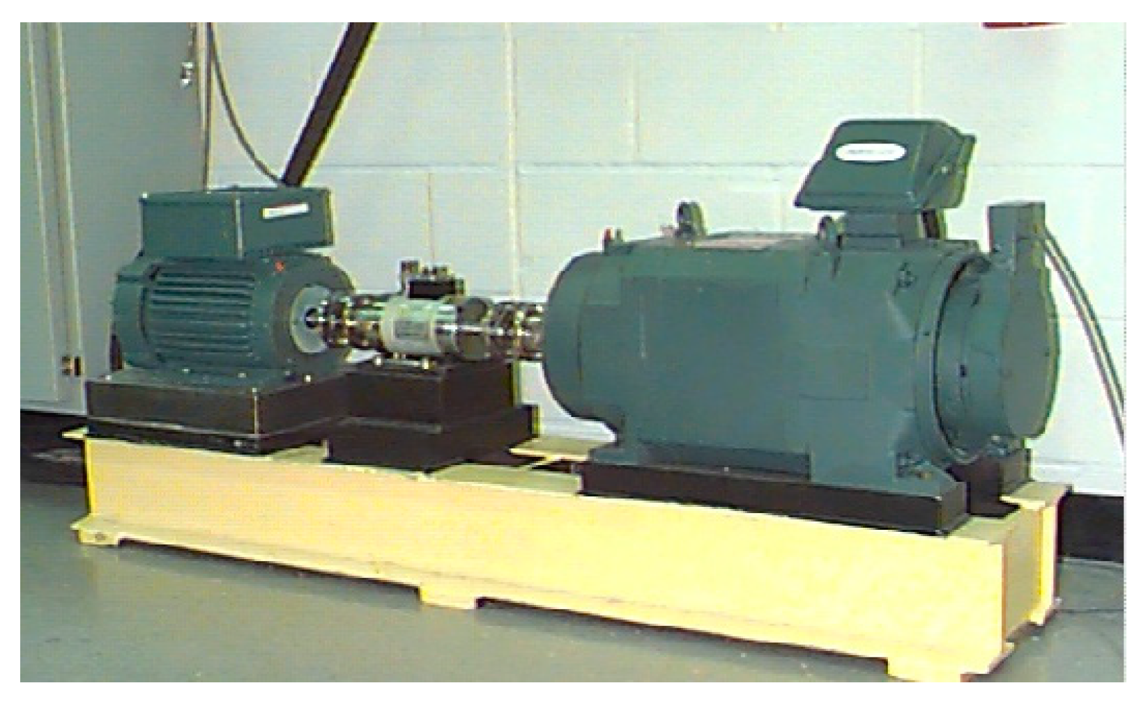
5. Case Study and Applicability Experiment

The objective of the experiment was to inspect if the fault feature IMFCM has superior fault diagnosis performance than the traditional features, both in abiding operating situations and hybrid operating situations. The vibration acceleration signal of the roller bearing is collected from the open source website of Case Western Reserve University whose vibration test platform is shown in Figure 3 [41]. The type of roller bearing is a deeply grooved ball bearing 6205-2RS JEM SKF whose outer ring is fixed with no guard. The format of size A × S × W is 25 mm × 52 mm × 15 mm, where A, S, and W represent aperture of inner ring, shaft diameter of outer ring, and width of roller bearing, respectively. The fault diameters of each fault style of inner ring fault, outer ring fault, and ball fault are 0.007 inches, 0.014 inches, and 0.021 inches, respectively, and the fault depth corresponding to each fault diameter is 0.11 inches. The outer ring fault location is 6 o’clock inside. The four fault styles are {normal, inner ring fault, outer ring fault, ball fault} which are represented by set {I, II, III, IV}. Experiments were conducted using a 2 HP Reliance Electric Motor, and the acceleration data was measured at locations near to the motor bearings.

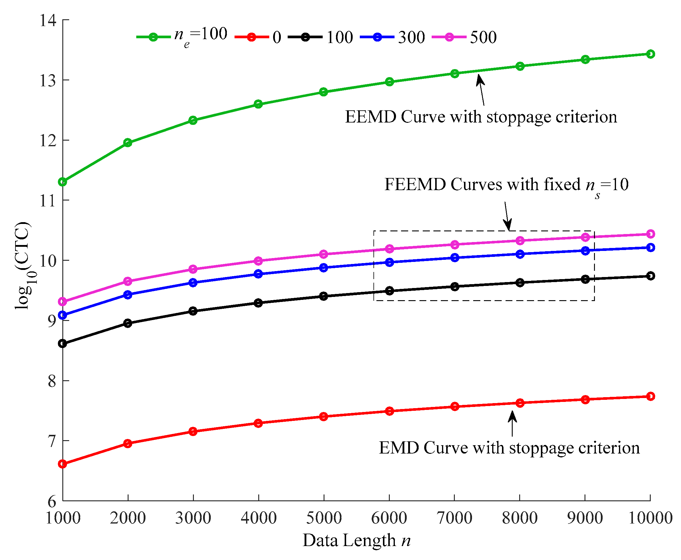
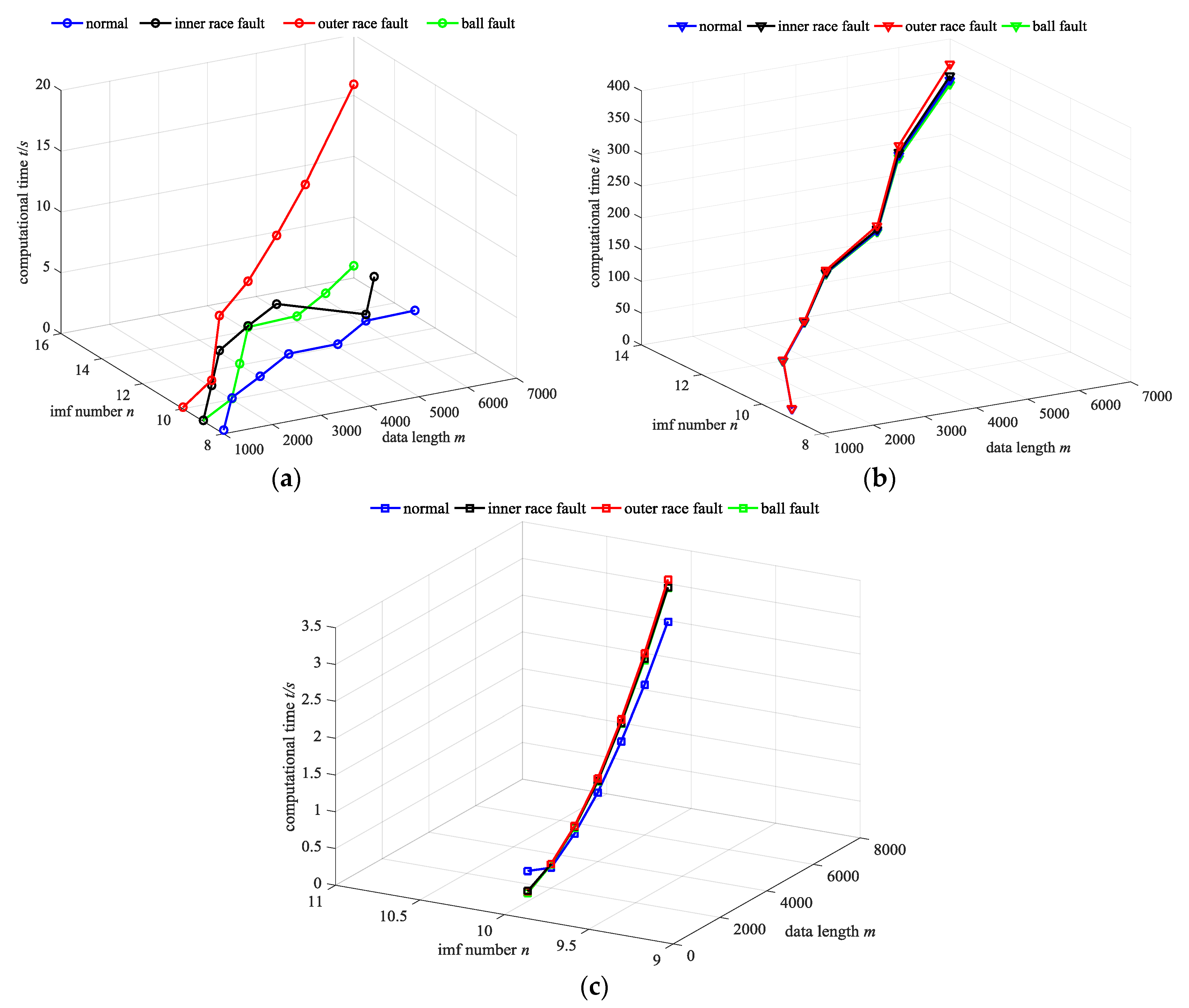
5.1. The Test of FEEMD Computational Time Complexity

First, we chose one vibration signal sample from each fault style of {I, II, III, IV} to check the computational time cost and the storage space cost of EMD, EEMD, and FEEMD. Figure 4 shows the relationship between the data length, IMF number, and the computing time cost of EMD, EEMD, and FEEMD. It is conceivable that FEEMD combines the advantages of EMD and EEMD, in that it computes faster than EEMD and weakens the mode mixing effect. The detailed computational time statistics are presented in Table 1, which shows the quantitative superiority of FEEMD. Figure 5 demonstrates the IMFs in time domain of EMD, EEMD, and FEEMD in a sample of roller bearing vibration signals for ball fault. Although the computing time is cut down, the IMFs still performed well compared with EMD and EEMD.

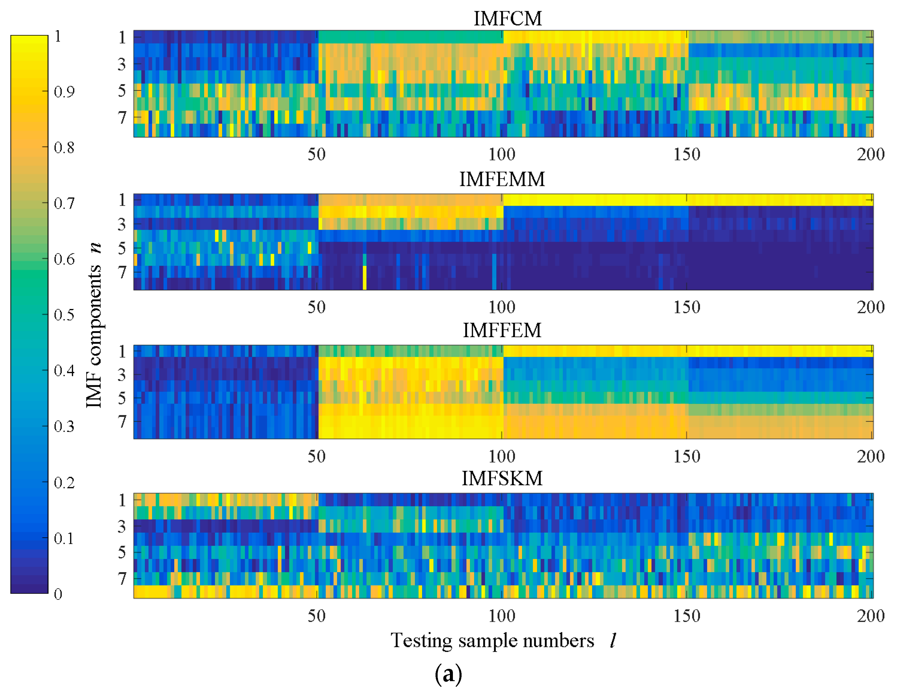
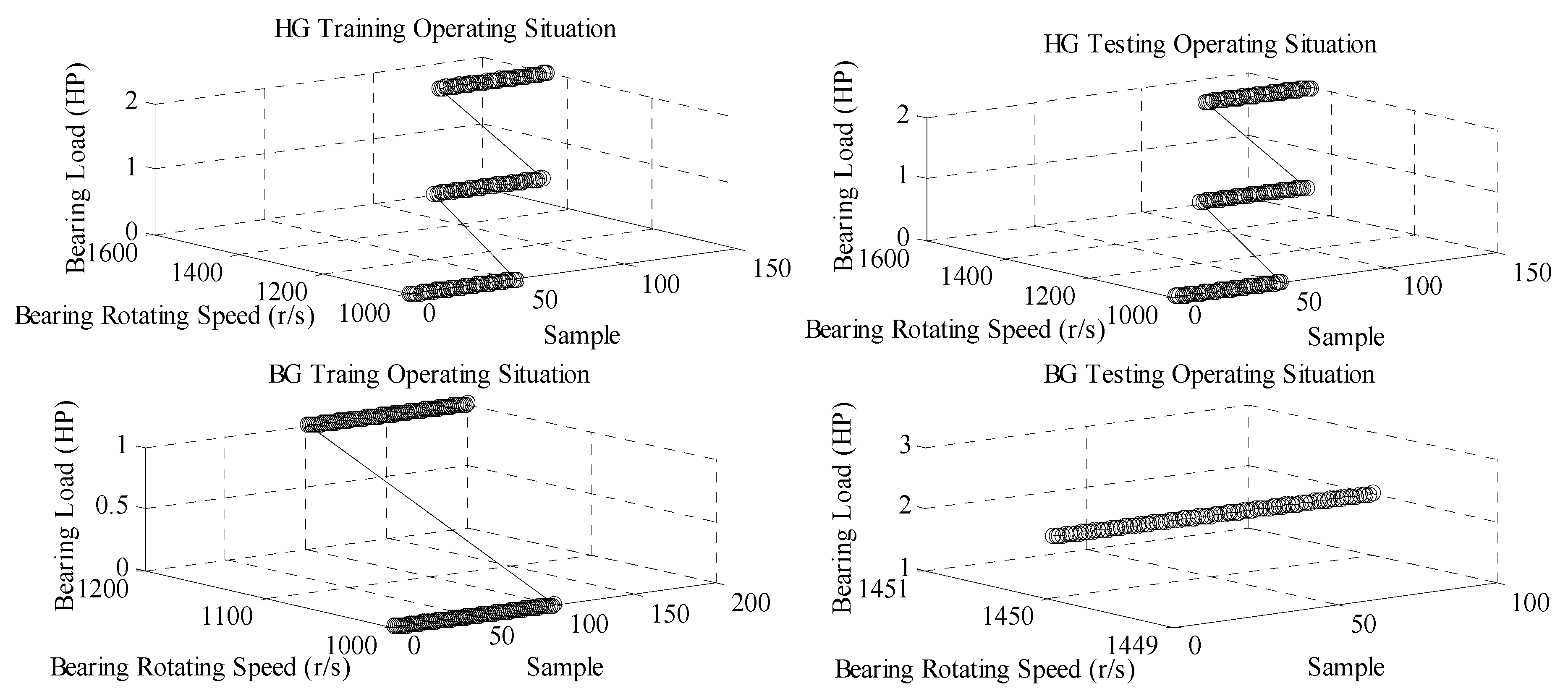
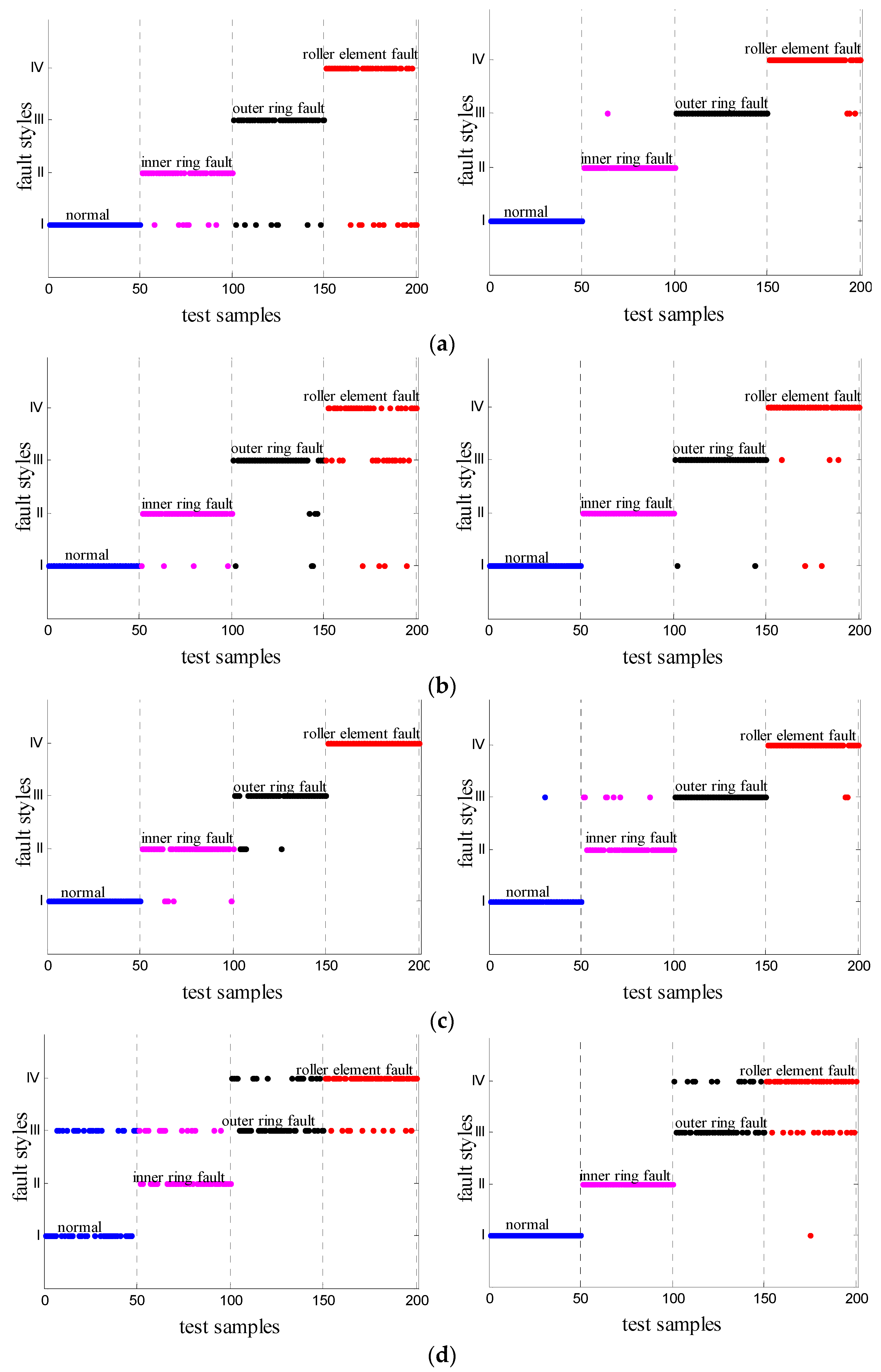
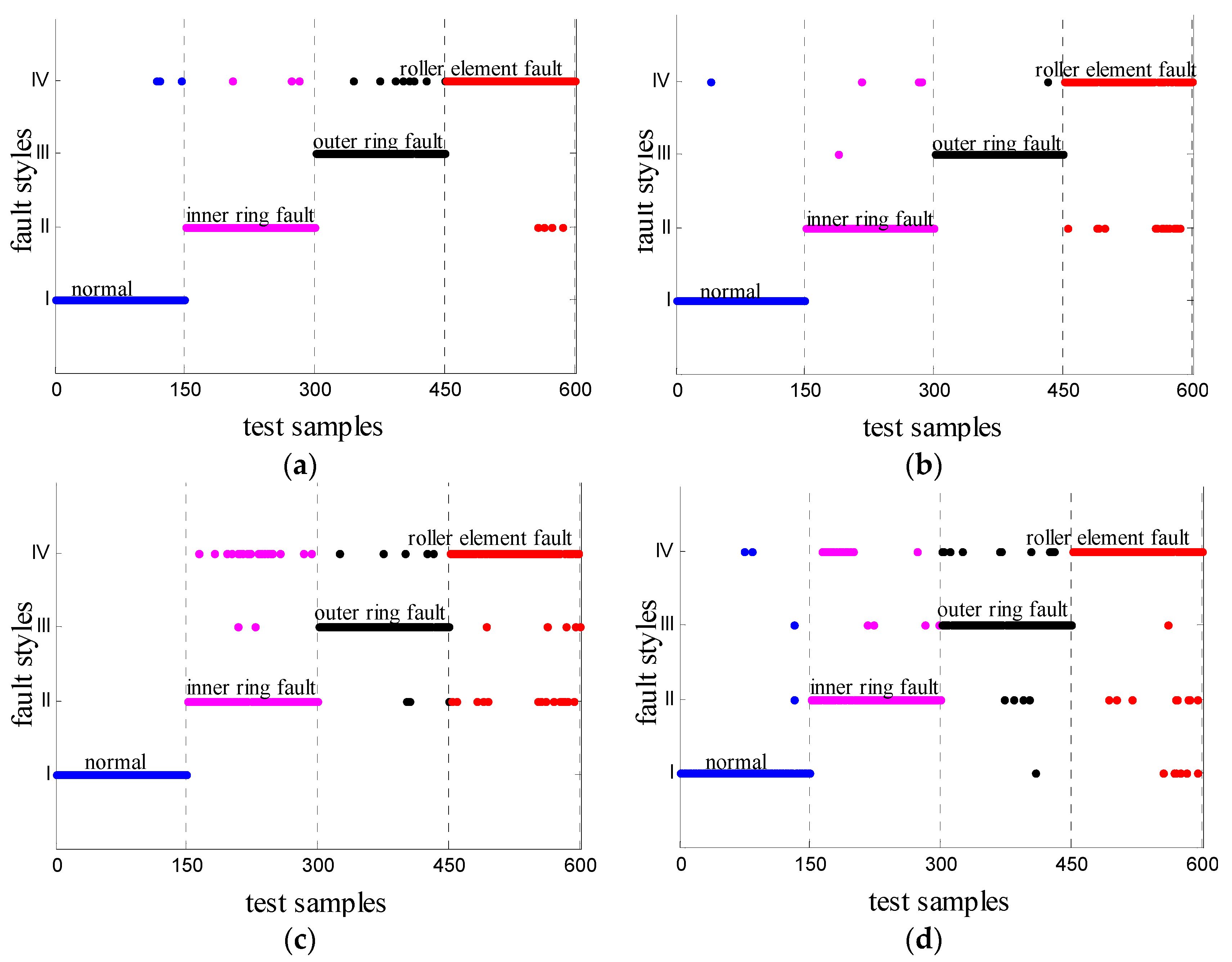
5.2. Stationary Operating Situations

Whatever operating situation the roller bearing is in, the matrix required for calculating the fault characteristic needs to be emphasized. For IMFCM, the dimensional value Γ: l × k × n needs to be solved, as well as the length m of each primary signal. Only if these parameters are cleared the high-dimensional experiment data can be conveniently calculated in blocks.
In this section, the fault diagnosis experiment of a roller bearing in a stationary operating situation is implemented. The experiment flow chart is provided in Figure 6 and the detailed steps are as follows.
Step one: data collection. The motor operating speed and load are constant. The roller bearing vibration data samples are distributed into three groups (A, B, and C) based on different operating parameters, each of which contains four fault styles of roller bearing expressed by {I, II, III, IV}. The roller bearing operating parameters are shown in Table 2. The sampling frequency is 12 kHz, under which 118 data sample sets have been obtained. Each data sample contains 1024 points. The training data sample number of each fault style is 68, and the testing data sample number is 50.
From the above information it is obvious that the total testing sample number is l = 200, the fault style number is k = 4, and the signal length m = 1024. The only parameter still unknown is the IMF number n for each primary signal.
Step two: time-frequency decomposition of vibration signal. Here, the primary signals of three groups are decomposed into IMF components by FEEMD. From Figure 5c it is obvious that the last two IMFs have little wave ingredients so that the meaningful IMFs contains only the first eight components.
Step three: feature extraction. Calculate IMFCM of the roller bearing vibration signal in each group according to the aforementioned process. To verify the fault diagnosis accuracy of IMFCM, the IMF energy moment matrix (IMFEMM) [42], IMF fuzzy entropy matrix (IMFFEM) [43], and IMF spectral kurtosis matrix (IMFSKM) [44] are considered as controlled objects which are extracted in the same process as the IMFCM, as shown in Figure 6. It is obvious that the features under the fourth component possess less feature diversity than the first four components in Figure 7 so they naturally have less contribution to the fault divisibility. Hence, component set {IMF1, IMF2, IMF3, IMF4} is chosen as the whole fault feature set for the roller bearing. Until now the parameters are all clear by l × k × n × m = 200 × 4 × 4 × 1024. By using the matrix form, the computation process will be intelligible and efficient.
Step four: fault identification. LSSVM has been proven to be a well-applied classifier when σ = 0.5 [40]. Here, the input set is made up of the four dimensions feature vectors acquired from step three, and the output set is vector [I, II, III, IV] signified [normal, inner ring fault, outer ring fault, ball fault]. The results of fault identification of the three fault severities are shown in Table 2, Table 3 and Table 4, in which CR θ, MR η, and AR μ are applied to evaluate the result quality.

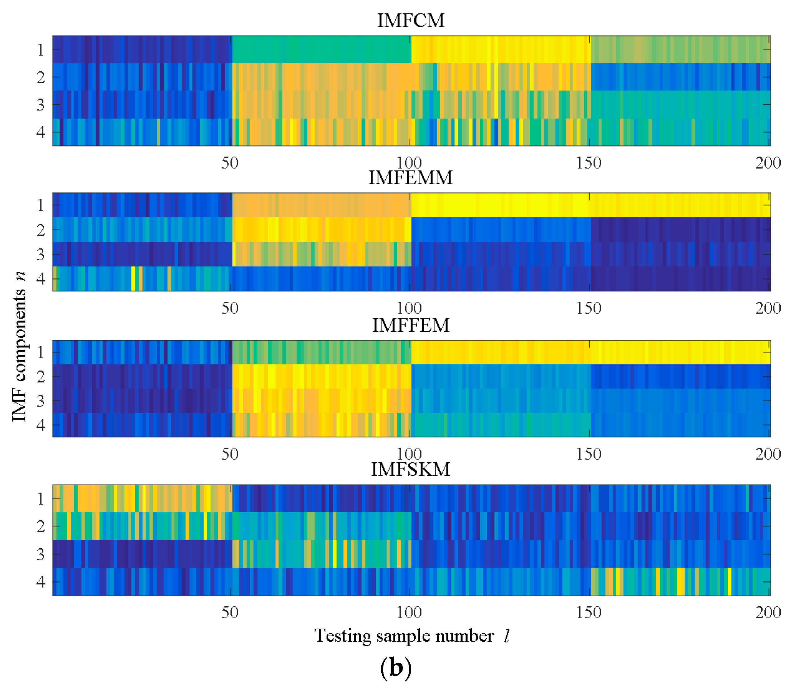
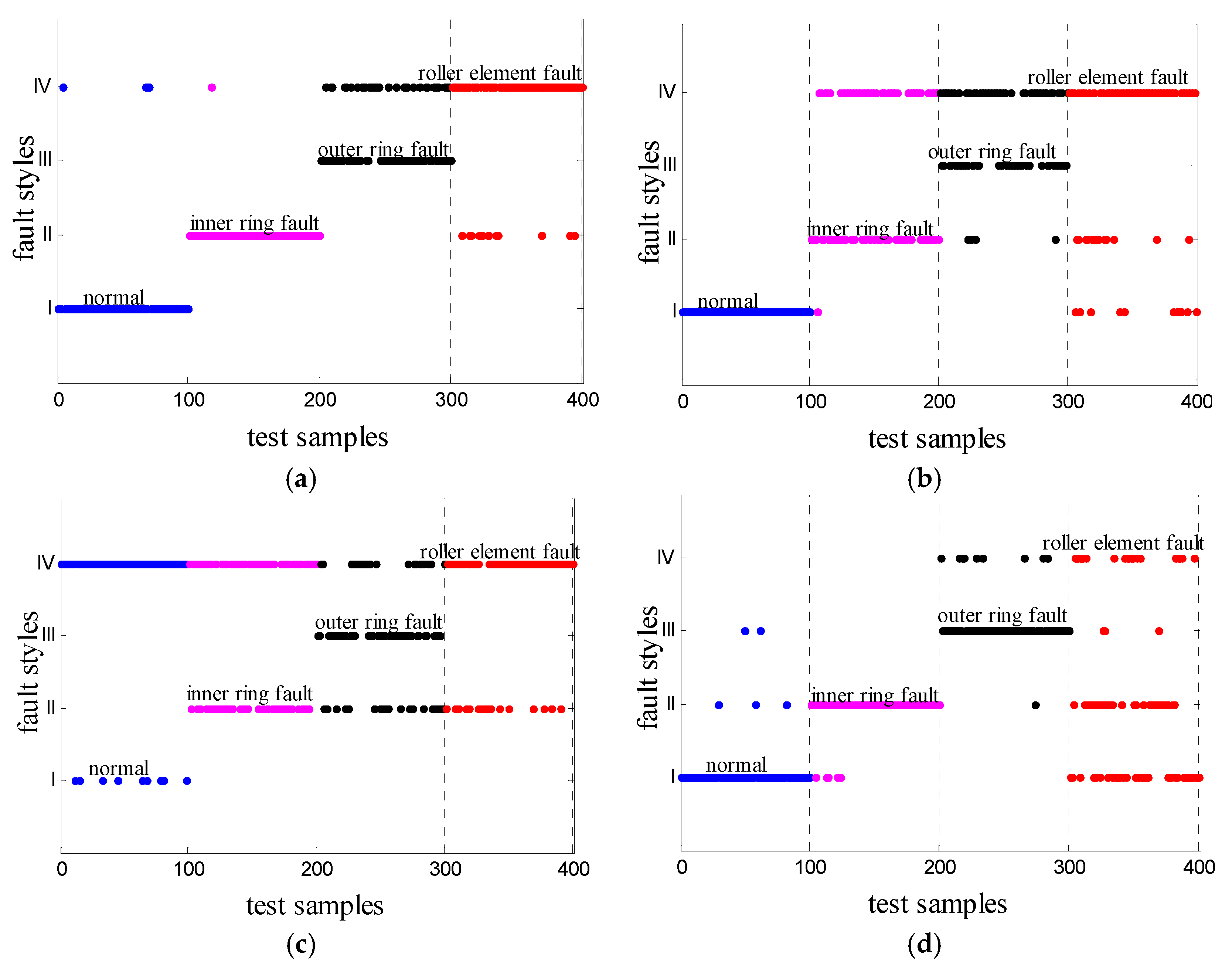
5.3. Cross-Mixed Operating Situations

The vibration data is the same as in Section 5.2. The purpose of the cross-mixed operating condition is to inspect the fault diagnosis robustness for the rotating condition of the IMFCM.
Step one: data extraction. Two hundred continuous samples are selected randomly from each roller bearing fault style dataset in group A, B, and C, respectively. The first 150 continuous samples of each fault style are intercepted, respectively, in group A, B, and C which are then mixed as a training set while another 150 samples from each group are designated as the testing set. As such, the total training set sample number is 450 with an equally sized testing set sample number. This fashion of cross-mixed rotating conditions follows the principle of distributing the training and testing dataset on the average of each group, which is called a Homogeneous Group (HG). Another method chooses 100 continuous samples of each fault style in group A and B both randomly as the training dataset, and 100 continuous samples of each fault style in group C as the testing dataset. This mixing fashion extracts the training dataset and testing dataset from different operating situations, respectively, so that it is called Biased Group (BG). The roller bearing operating parameter distributions in HG and BG are shown in Figure 8.
Step two: To execute FEEMD, feature extraction, and intelligent identification processes in turn. The procedure is the same as steps two and three provided in Section 5.2.
Step three: To compare the test performances and explain the consequences.

6. Discussion

From Figure 4 and Table 1, it can be concluded intuitively that the calculation time cost of FEEMD is the least of the three algorithms. Furthermore, FEEMD can obtain a constant number of IMF so that it shows stable decomposition process. Additionally, the results of FEEMD are as good as those of EEMD, to which it is compared in Figure 5.
Analyzing Figure 7, the first four-dimensional CM, EMM, FEM, and SKM are all stable, and have obvious diversity among different fault styles. However, the last four-dimensional CM, EMM, FEM, and SKM are unstable and own ledivisibility relatively. Hence, it can be concluded qualitatively that to obtain accurate fault identification results, the last four-dimensional feature should be moved from the feature matrix. Furthermore, Figure 9 shows the quantitative comparison of the four features based on the samples of the 0.007 inches ball fault data from Group A. The results shown in Figure 9 are the LSSVM outputs. The identification results in Figure 9 indicate that the diagnosis accuracy of the first four dimensional feature matrix is higher than the eight dimensional feature matrix. Therefore, it is the first four dimensional IMFs that perform as the more effective feature matrix. The dimension of the testing set is 200 × 4 × 4 × 1024.
The roller bearing fault diagnosis results of the three fault diameters (0.007 inches, 0.014 inches, and 0.021 inches) are revealed in Table 3, Table 4 and Table 5. The diagnosis accuracy of SKM were less than CM, EMM, and FEM as reflected by θ. Corresponding to column “I”, the misdiagnosis rate η of non-normal data is the key reference for reliability in engineering applications. Through contrasting the four features, CM and FEM were observed to have a value of zero for η in all the tests of Table 3, Table 4 and Table 5; as such, CM and FEM are qualified to measure the reliability of roller bearings. μ reflects the average diagnosis ability. Having μ values for all the features above 85% means that CM, EMM, FEM, and SKM are capable of implementing roller bearing fault diagnosis work.
To summarize what is mentioned above, under the stationary operation condition, CM as the fault feature has almost the same diagnosis ability with EMM and FEM, and is better than SKM. Meanwhile, CM can prevent the fault data from misdiagnosing into the normal state, and thus it can provide the reliability of the application to the roller bearing.
Figure 10 and Figure 11 present the intuitive fault diagnosis results based on LSSVM, and Table 6, Table 7, Table 8, Table 9, Table 10 and Table 11 show the exhaustive quantified results. In analyzing the results, several conclusions can be discovered. CM is the only feature that maintains high accuracy of three fault diameter conditions in group HG and BG. However, the diagnosis accuracy of SKM in each condition is not good enough to implement the fault identification (i.e., SKM has no qualification to diagnose fault of roller bearings in non-stationary operating conditions). With the increase of the fault diameter, the fault diagnosis accuracy of each feature decreases, especially for EMM and FEM. More specifically, CM is sensitive not only to the light faults but deep faults, while EMM and FEM are exceedingly sensitive to light faults and are insensitive to deep faults. In terms of BG, it generates lower diagnosis accuracy for EMM and FEM than HG. This can be explained in that the feature distribution is not balanced in each operating situation of EMM and FEM. Nevertheless, that phenomenon which is weakened by CM proves that CM has the robustness for fault identification in various operating situations. Although the AR μ of CM in Table 10 and Table 11 decreased to below 90%, the normal state in each fault diameter condition has been well recognized, and is better than the other features. This proves that correntropy is sensitive to shock response.
All in all, the results verify that CM is the only feature that possesses both the robustness and the high diagnosis accuracy in a variety of different operating situations.

7. Conclusions

In order to extract the fault feature and recognize the fault pattern of bearing vibration signals, this paper proposes a novel approach combining the FEEMD, IMFCM, and LSSVM methods. The analysis results from the simulation signal and the experiment data demonstrate the superiority of the approach presented by this paper.
Compared with EMD and EEMD, the test result of FEEMD shows the two advantages, namely the faster computation time and the avoidance of the mode mixing effect. The FEEMD-IMFCM-LSSVM approach framework is proposed here to achieve roller bearing fault identification both in stationary and non-stationary operating situations. Bearing rotating speed and load were the changing operating parameters considered by this paper. The IMFCM was extracted from the IMF component that was decomposed from the roller bearing vibration signal by FEEMD. Exhaustively, it is through the AM-correntropy mathematical model of primary vibration signal and IMF components that IMFCM could be obtained.
Through experiments considering single and cross-mixed operating situations, IMFEMM, IMFFEM, and IMFSKM were compared in their ability to diagnose roller bearing faults. The compared diagnosis results verify that IMFCM has the highest fault divisibility and robustness of its operating state in both single and mixed operating conditions. To be expanded for further consideration, the identification of roller bearing damage degree has great significance in improving the ability of fault warnings. In the future, the application of IMFCM could focus on performance degradation detection and identification of the degree of damage to rotary machines.

Acknowledgments

The authors would like to express their appreciation to the editor and anonymous reviewers for their help in revising the manuscript. The support of Key Technologies R&D Program of China I16B300011 and State Key Laboratory independent project of Beijing Jiaotong University I16K00100 are also gratefully acknowledged.

Author Contributions

The thought process behind the design of this method was put forward by Limin Jia and Yunxiao Fu; Yunxiao Fu, Limin Jia, Yong Qin and Jie Yang were in charge of the experimental implementation and manuscript writing; Ding Fu was in charge of the data analysis and manuscript modification. All the authors have read and approved the final manuscript.

Conflicts of Interest

The authors declare no conflict of interest.

References

  1. Tabrizi, A.; Garibaldi, L.; Fasana, A. Early damage detection of roller bearings using wavelet packet decomposition, ensemble empirical mode decomposition and support vector machine. Meccanica 2015, 50, 865–874. [Google Scholar] [CrossRef]
  2. Frosini, L.; Harlisca, C.; Szabó, L. Induction machine bearing faults detection by means of statistical processing of the stray flux measurement. IEEE Trans. Ind. Electron. 2015, 62, 1846–1854. [Google Scholar] [CrossRef]
  3. Dalvand, F.; Keshavarzi, M.; Kalantar, A.; Cheraghar, A. Detection of generalized-roughness bearing fault using statistical-time indices of instantaneous frequency of motor voltage space vector. In Proceedings of the 23rd Iranian Conference on Electrical Engineering (ICEE’ 2015), Tehran, Iran, 10–14 May 2015; pp. 1516–1521.
  4. Renaudin, L.; Bonnardot, F.; Musy, O.; Doray, J.B.; Rémond, D. Natural roller bearing fault detection by angular measurement of true instantaneous angular speed. Mech. Syst. Signal Process. 2010, 24, 1998–2011. [Google Scholar] [CrossRef]
  5. Zhong, B.L.; Huang, R. Introduction to Machine Fault Diagnosis, 3rd ed.; China Machine Press: Beijing, China, 2007; pp. 1–16. [Google Scholar]
  6. Lim, G.M.; Bae, D.M.; Kim, J.K. Fault diagnosis of rotating machine by thermography method on support vector machine. J. Mech. Sci. Technol. 2014, 28, 2947–2952. [Google Scholar] [CrossRef]
  7. Rai, V.K.; Mohanty, A.R. Bearing fault diagnosis using FFT of intrinsic mode functions in Hilbert–Huang transform. Mech. Syst. Signal Process. 2007, 21, 2607–2615. [Google Scholar] [CrossRef]
  8. Yu, Y.; Yu, D.J.; Cheng, J.S. A roller bearing fault diagnosis method based on EMD energy entropy and ANN. J. Sound Vib. 2006, 204, 269–277. [Google Scholar] [CrossRef]
  9. Huang, N.E.; Shen, Z.; Long, S.R. The Empirical mode decomposition and the Hilbert spectrum for nonlinear and non-stationary time series analysis. Proc. R. Soc. Lond. A 1998, 454, 903–995. [Google Scholar] [CrossRef]
  10. Han, M.H.; Pan, J.L. A fault diagnosis method combined with FEEMD, sample entropy and energy ratio for roller bearings. Measurement 2015, 75, 7–19. [Google Scholar] [CrossRef]
  11. Huang, N.E.; Shen, Z.; Long, S.R. A New View of Nonlinear Water Waves the Hilbert Spectrum. Annu. Rev. Fluid Mech. 1999, 31, 417–467. [Google Scholar] [CrossRef]
  12. Wu, Z.H.; Huang, N.E. Ensemble Empirical Mode Decomposition a Noise-assisted Data Analysis Method. Adv. Adapt. Data Anal. 2009, 1, 1–41. [Google Scholar] [CrossRef]
  13. Wei, G.; Tse, P.W. A novel signal compression method based on optimal ensemble empirical mode decomposition for bearing vibration signals. J. Sound Vib. 2013, 332, 423–441. [Google Scholar]
  14. Xue, X.M.; Zhou, J.Z.; Xu, Y.H.; Zhu, W.L.; Li, C.C. An adaptively fast ensemble empirical mode decomposition method and its applications to rolling element bearing fault diagnosis. Mech. Syst. Signal Process. 2015, 62–63, 444–459. [Google Scholar] [CrossRef]
  15. Wang, Y.H.; Yeha, C.H.; Young, H.V.; Hu, K.; Lo, M.T. On the computational complexity of the empirical mode decomposition algorithm. Physica A 2014, 390, 159–167. [Google Scholar] [CrossRef]
  16. Liu, H.; Tian, H.Q.; Liang, X.F.; Li, Y.F. New wind speed forecasting approaches using fast ensemble empirical model decomposition, genetic algorithm, Mind Evolutionary Algorithm and Artificial Neural Networks. Renew. Energy 2015, 83, 1066–1075. [Google Scholar] [CrossRef]
  17. Shi, Z.L.; Song, W.Q.; Taheri, S. Improved LMD, Permutation Entropy and Optimized K-Means to Fault Diagnosis for Roller Bearings. Entropy 2016, 18, 70. [Google Scholar] [CrossRef]
  18. Hsieh, N.K.; Lin, W.Y.; Young, H.T. High-Speed Spindle Fault Diagnosis with the Empirical Mode Decomposition and Multiscale Entropy Method. Entropy 2015, 17, 2170–2183. [Google Scholar] [CrossRef]
  19. Bishara, A.J.; Hittner, J.B. Reducing Bias and Error in the Correlation Coefficient Due to Non-normality. Educ. Psychol. Meas. 2015, 75, 785–804. [Google Scholar] [CrossRef]
  20. Xu, W.C.; Chang, C.Q.; Hung, Y.S.; Fung, P.C.W. Asymptotic Properties of Order Statistics Correlation Coefficient in the Normal Cases. IEEE Trans. Signal Process. 2008, 56, 2239–2248. [Google Scholar] [Green Version]
  21. Puth, M.T.; Neuhäuser, M.; Ruxton, G.D. Effective use of Spearman’s and Kendall’s correlation coefficients for association between two measured traits. Anim. Behav. 2015, 102, 77–84. [Google Scholar] [CrossRef]
  22. Li, J.W.; Qian, H.D. Correntropy method for spectrum estimation in impulsive noise environment. Signal Process. 2014, 30, 944–948. [Google Scholar]
  23. Santamaria, I.; Pokharel, P.P.; Principe, J.C. Generalized correlation function: Definition, properties, and application to blind equalization. IEEE Trans. Signal Process. 2006, 54, 2187–2197. [Google Scholar] [CrossRef]
  24. Gunduz, A.; Principe, J.C. Correntropy as a novel measure for nonlinearity tests. Signal Process. 2009, 89, 14–23. [Google Scholar] [CrossRef]
  25. Xing, H.J.; Ren, H.R. Regularized correntropy criterion based feature extraction for novelty detection. Neurocomputing 2014, 133, 483–490. [Google Scholar] [CrossRef]
  26. Wang, Y.; Pan, C.H.; Xiang, S.M.; Zhu, F.Y. Robust hyper spectral unmixing with correntropy-based metric. IEEE Trans. Image Process. 2015, 24, 3927–3939. [Google Scholar]
  27. Zhang, Z.J.; Chen, J.H. Correntropy based data reconciliation and gross error detection and identification for nonlinear dynamic processes. Comput. Chem. Eng. 2015, 75, 120–134. [Google Scholar] [CrossRef]
  28. Hassan, M.; Terrien, J.; Marque, C.; Karlsson, B. Comparison between approximate entropy, correntropy and time reversibility: Application to uterine electromyogram signals. Med. Eng. Phys. 2011, 33, 980–986. [Google Scholar] [CrossRef] [PubMed]
  29. Zhang, X.Y.; Zhou, J.Z. Multi-fault diagnosis for rolling element bearings based on ensemble empirical mode decomposition and optimized support vector machines. Mech. Syst. Signal Process. 2013, 41, 127–139. [Google Scholar] [CrossRef]
  30. Wan, Y.; Wu, C.W. LSSVM Algorithm and Its Application Research in Non-Linear Reliability Identification. Adv. Sci. Lett. 2012, 6, 464–467. [Google Scholar] [CrossRef]
  31. Jiang, F.; Zhu, Z.C.; Li, W.; Zhou, G.B.; Chen, G. Fault identification of rotor-bearing system based on ensemble empirical mode decomposition and self-zero space projection analysis. J. Sound Vib. 2014, 333, 3321–3331. [Google Scholar] [CrossRef]
  32. Penga, Z.K.; Tseb, P.W.; Chu, F.L. An improved Hilbert–Huang transform and its application in vibration signal analysis. J. Sound Vib. 2005, 286, 187–205. [Google Scholar] [CrossRef]
  33. Rilling, G.; Flandrin, P.; Gonçalvés, P. On Empirical Mode Decomposition and Its Algorithms. In Proceedings of the 3rd IEEE-EURASIP Workshop on Nonlinear Signal and Image Processing, Grado, Italy, 8–11 June 2003.
  34. Cheng, J.S.; Yu, D.J.; Yang, Y. Research on the Intrinsic Mode Function (IMF) Criterion in EMD Method. Mech. Syst. Signal Process. 2005, 20, 817–824. [Google Scholar]
  35. Sun, W.; Liu, M.H.; Liang, Y. Wind Speed Forecasting Based on FEEMD and LSSVM Optimized by the Bat Algorithm. Energies 2015, 8, 6585–6607. [Google Scholar] [CrossRef]
  36. Wu, Z.H.; Huang, N.E. On the filtering properties of the empirical mode decomposition. Adv. Adapt. Data Anal. 2010, 2, 397–414. [Google Scholar] [CrossRef]
  37. Wang, J.J.; Wang, Y.J.; Jing, B.Y.; Gao, X. Regularized maximum correntropy machine. Neurocomputing 2015, 16, 85–92. [Google Scholar] [CrossRef]
  38. Yang, Y.; Yu, D.J.; Cheng, J.S. A Fault Diagnosis approach for roller bearing based on IMF envelope spectrum and SVM. Measurement 2007, 39, 943–950. [Google Scholar] [CrossRef]
  39. Suykens, J.A.K.; Vandewalle, J. Least squares support vector machine classifiers. Neural Process. Lett. 1999, 9, 293–300. [Google Scholar] [CrossRef]
  40. Zhang, Y.; Qin, Y.; Xing, Z.Y.; Jia, L.M.; Cheng, X.Q. Roller bearing safety region estimation and state identification based on LMD–PCA–LSSVM. Measurement 2013, 46, 1315–1324. [Google Scholar] [CrossRef]
  41. Case Western Reserve University Bearing Data Center. Available online: http://csegroups.case.edu/bearingdatacenter/home (accessed on 23 June 2016).
  42. Bin, G.F.; Gao, J.J.; Li, X.J.; Dhillon, B.S. Early fault diagnosis of rotating machinery based on wavelet packets—Empirical mode decomposition feature extraction and neural network. Mech. Syst. Signal Process. 2012, 27, 696–711. [Google Scholar] [CrossRef]
  43. Li, Y.B.; Xu, M.Q.; Zhao, H.Y.; Huang, W. Hierarchical fuzzy entropy and improved support vector machine based binary tree approach for rolling bearing fault diagnosis. Mech. Mach. Theory 2016, 98, 114–132. [Google Scholar] [CrossRef]
  44. Tian, J.; Morillo, C.; Azarian, M.H.; Pecht, M. Motor Bearing Fault Detection Using Spectral Kurtosis-Based Feature Extraction Coupled With K-Nearest Neighbor Distance Analysis. IEEE Trans. Ind. Electron. 2016, 63, 1793–1803. [Google Scholar] [CrossRef]
Figure 1. Roller bearing fault diagnosis method based on FEEMD-IMFCM-LSSVM. FEEMD: Fast Ensemble Empirical mode decomposition; IMF: Intrinsic Mode Functions; IMFCM: IMF correntropy matrix; LSSVM: Least Square Support Vector Machine.
Entropy 18 00242 g001
Figure 2. The curve of log10(CTC) versus data length m. CTC: Computational Time Complexity; EMD: Empirical Mode Decomposition; EEMD: Ensemble Empirical Mode Decomposition.
Entropy 18 00242 g002
Figure 3. Roller bearing vibration test rig.
Entropy 18 00242 g003
Figure 4. The relationship curve of the data length, IMF number and computational time. (a) EMD algorithm; (b) EEMD algorithm; (c) fast EEMD algorithm.
Entropy 18 00242 g004
Figure 5. View of inner race fault bearing signal IMFs in A group of 0.007 inches fault diameter. (a) Inner race fault signal IMFs by EMD in A group; (b) Inner race fault signal IMFs by EEMD in A group; (c) Inner race fault signal IMFs by FEEMD in A group.
Entropy 18 00242 g005aEntropy 18 00242 g005b
Figure 6. FEEMD-IMFCM-LSSVM roller bearing fault identification experiment flow diagram.
Entropy 18 00242 g006
Figure 7. Chromatogram of the eight and four dimensional Feature Matrixes in A Group (0.007 inches fault diameter). (a) Eight-IMF feature matrix; (b) Eight-IMF feature matrix.
Entropy 18 00242 g007aEntropy 18 00242 g007b
Figure 8. Rotating speed and load distribution in training and testing sample sets of HG and BG.
Entropy 18 00242 g008
Figure 9. Dimension reduction superiority for feature matrixes reflected in classification results of A Group. (a) IMFCM classification result comparison between eight-IMF and four-IMF; (b) IMF energy moment matrix (IMFEMM) classification result comparison between eight-IMF and four-IMF; (c) IMF fuzzy entropy matrix (IMFFEM) classification result comparison between eight-IMF and four-IMF; (d) IMF spectral kurtosis matrix (IMFSKM) classification result comparison between eight-IMF and four-IMF.
Entropy 18 00242 g009
Figure 10. Fault identification result of Homogeneous Group (0.014 inches). (a) IMFCM; (b) IMFEMM; (c) IMFFEM; (d) IMFSKM.
Entropy 18 00242 g010
Figure 11. Fault identification result of Bias group (0.021 inches). (a) IMFCM; (b) IMFEMM; (c) IMFFEM; (d) IMFSKM.
Entropy 18 00242 g011
Table 1. Computational time statistics.
Fault StyleAlgorithmLength of Data
1000200030003900500060007000
NormalEMD0.3440.0620.0860.1410.1640.2500.297
EEMD5.90910.91921.10735.92354.90384.121122.927
FEEMD0.2820.2190.4380.7191.1081.5462.103
Inner Race FaultEMD0.0620.0630.1410.2810.3120.6410.859
EEMD5.71111.15621.36336.37956.06586.945126.945
FEEMD0.1250.250.50.8281.2821.7972.466
Outer Race FaultEMD0.0780.4222.3153.1044.556.39512.31
EEMD5.71311.41621.9437.65958.49591.396134.166
FEEMD0.0940.2660.50.8441.3131.8592.5360
Ball FaultEMD0.0940.250.4840.8281.2651.8132.44
EEMD5.53910.95220.9635.44154.699 85.544122.701
FEEMD0.0310.0460.1090.1880.3440.3970.797
Table 2. Operating parameters for the A, B, and C groups.
Operating ParametersA GroupB GroupC Group
Speed1750 r/min1772 r/min1797 r/min
Load2HP1HP0
Table 3. Fault diagnosis result comparison of 0.007 inches fault diameter.
EvaluationFeature A Group: 1750 r/min & 2HPB Group: 1772 r/min & 1HPC Group: 1797 r/min & 0HP
IIIIIIIVIIIIIIIVIIIIIIIV
θ (%)CM1009810094100961009498 90100100
EMM100100969010010096981009810096
FEM9886100961001001009810010010094
SKM1001007470100100769494929492
η (%)CM000.270003.3300040
EMM2.6702001.330.670.910.6701.330
FEM006.670000.6700020
SKM0.6709.338.671.330.67260.674.6704
μ (%)CM9897.597
EMM96.598.598.5
FEM9599.598.5
SKM8692.593
I is normal state, II is inner ring fault, III is outer ring fault, and IV is ball fault, the same as all the following tables.
Table 4. Fault diagnosis result comparison of 0.014 inches fault diameter.
EvaluationFeatureA Group: 1750 r/min & 2HPB Group: 1772 r/min & 1HPC Group: 1797 r/min & 0HP
IIIIIIIVIIIIIIIVIIIIIIIIV
θ(%)CM98 9892100100969610096 929498
EMM1001009888100989092100869888
FEM100849898100929898100969492
SKM9478969810082909892808290
η (%)CM00040002.6701.3305.33
EMM40.67000.682.673.3303.330.6705.33
FEM00.670601.332.67001.3322.67
SKM00.67010.6701.332.676206.6710
μ (%)CM979895
EMM96.59593
FEM959795.5
SKM91.592.586
Table 5. Fault diagnosis result comparison of 0.021 inches fault diameter.
EvaluationFeatureA Group: 1750 r/min & 2HPB Group: 1772 r/min & 1HPC Group: 1797 r/min & 0HP
IIIIIIIVIIIIIIIVIIIIIIV
θ (%)CM100901009810094988698 9610088
EMM9810010010010010010092929810096
FEM10096100100100961008410010010096
SKM98761009898921009886789682
η (%)CM004001.33600060
EMM000.670002.670004.670
FEM001.330006.670001.330
SKM00.671.337.330102.671.334.671.333.3310
μ (%)CM9794.595.5
EMM99.59896.5
FEM939599
SKM91.589.585.5
Table 6. Fault diagnosis result comparison in Homogeneous Group (0.007 inches).
Feature IndexHomogeneous Group
IIIIIIIVμ (%)
θ (%)η (%)θ (%)η (%)θ (%)η (%)θ (%)η (%)
CM99.33097.3301002.6795.33098
EMM1000.8999.330980.4496.670.6798.5
FEM1000100099.330.4498.670.2299.5
SKM97.331.11961.78854826.2290.17
Table 7. Fault diagnosis result comparison in Homogeneous Group (0.014 inches).
Feature IndexHomogeneous Group
IIIIIIIVμ (%)
θ (%)η (%)θ (%)η (%)θ (%)η (%)θ (%)η (%)
CM98 0980.8994.67097.333.1197
EMM99.33096499.330.22880.15695.67
FEM100 0844.8994.671.5684690.67
SKM97.33 1.56843.1189.331.5689.337.1190
Table 8. Fault diagnosis result comparison in Homogeneous Group (0.021 inches).
Feature IndexHomogeneous Group
IIIIIIIVμ (%)
θ (%)η (%)θ (%)η (%)θ (%)η (%)θ (%)η (%)
CM98.67 091.333.11903.1199.330.6794.83
EMM99.33099.3301001.3397.33099
FEM100 099.3301000.4499.33099.67
SKM88.67 1.1183.33486.67492.677.1187.83
Table 9. Fault diagnosis result comparison in Biased Group (0.007 inches).
Feature IndexBiased Group
IIIIIIIVμ (%)
θ (%)η (%)θ (%)η (%)θ (%)η (%)θ (%)η (%)
CM9609301007.3389094.5
EMM1001.67990.679622.33281080.75
FEM42010019.33998.33750.3379
SKM95159513.33881.67213.6774.75
Table 10. Fault diagnosis result comparison in Biased Group (0.014 inches).
Feature IndexBiased Group
IIIIIIIVμ (%)
θ (%)η (%)θ (%)η (%)θ (%)η (%)θ (%)η (%)
CM970993.67650891.387.5
EMM1004.675264207333.6766.75
FEM903914.674707960.3343.75
SKM3 07212.333573.336754.6744.25
Table 11. Fault diagnosis result comparison in Biased Group (0.021 inches).
Feature IndexBiased Group
IIIIIIIVμ (%)
θ (%)η (%)θ (%)η (%)θ (%)η (%)θ (%)η (%)
CM1000760.6710020.3361084.25
EMM9900010035.3395073.5
FEM1000010063.6799052.25
SKM00893.679778133.6766.75

