
A Simulation-Based Study on Bayesian Estimators for the Skew Brownian Motion


Abstract
:
1. Introduction
2. Model Formulation
2.1. Skew Brownian Motion
- X is adapted to the filtration , where ;
- X is a continuous process;
- ;
- with probability one, we have .
2.2. Transition Probabilities
2.3. Exiting Times
3. Bayesian Inference
3.1. Likelihood and Prior Settings
3.2. Hypotheses Testing
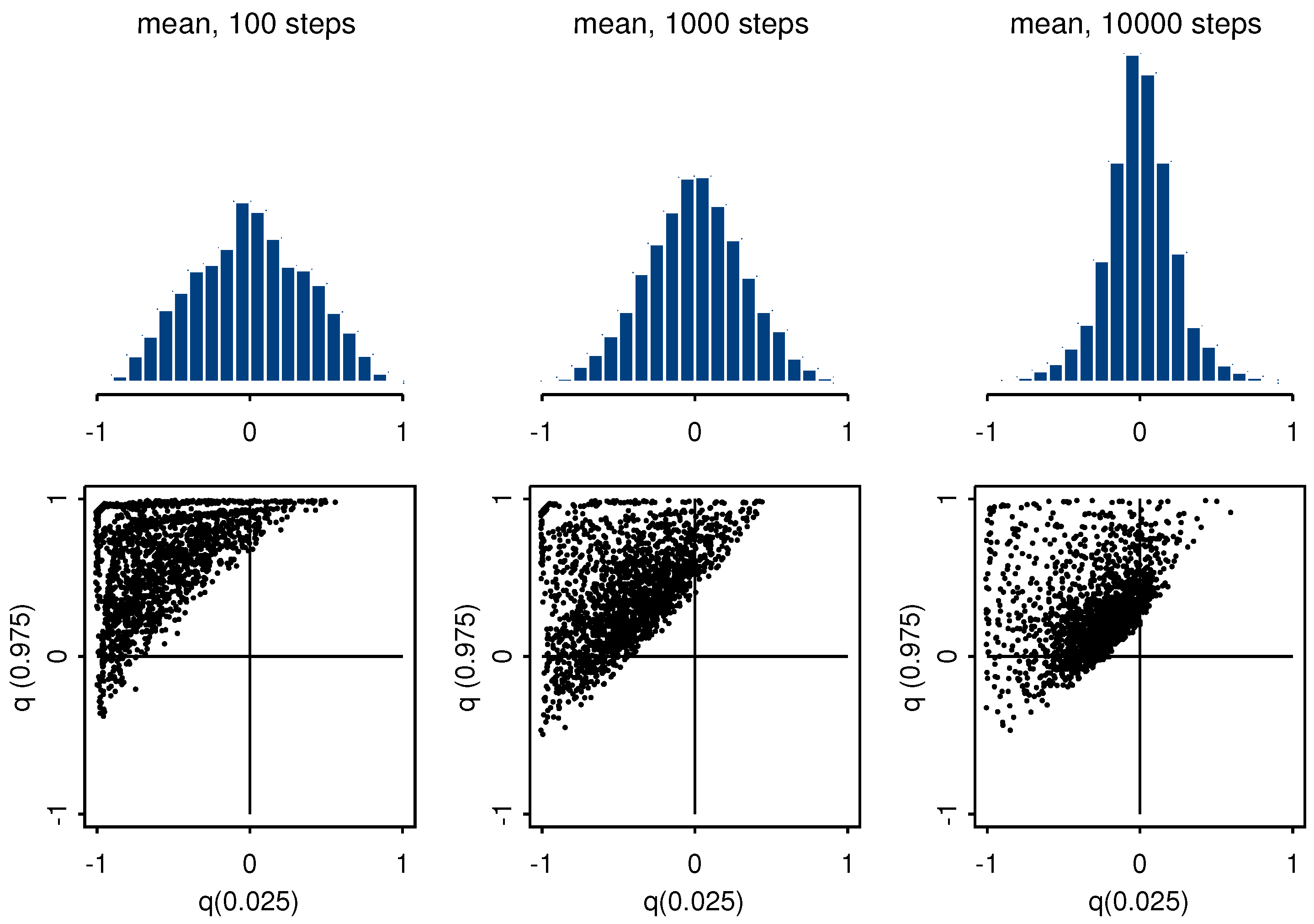
3.3. Considerations on the Asymptotic Behavior of the Bayesian Posterior
4. Computation for Data
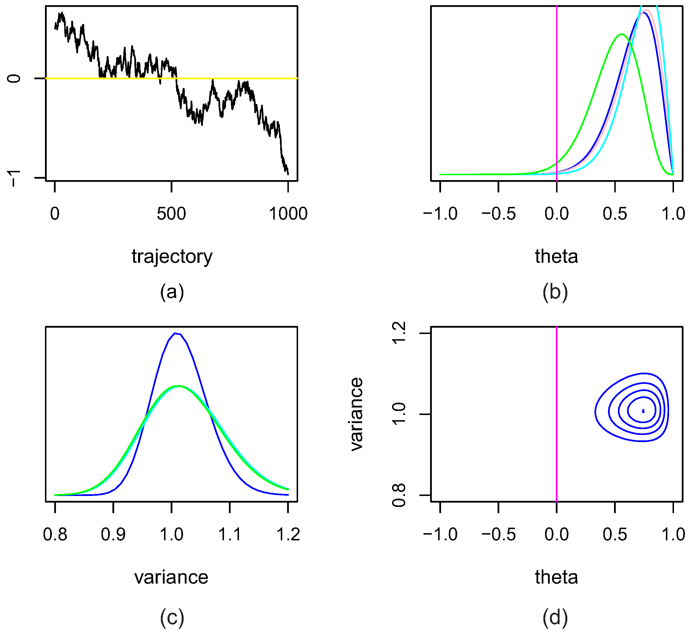
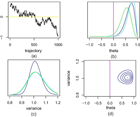
4.1. Simulated Data
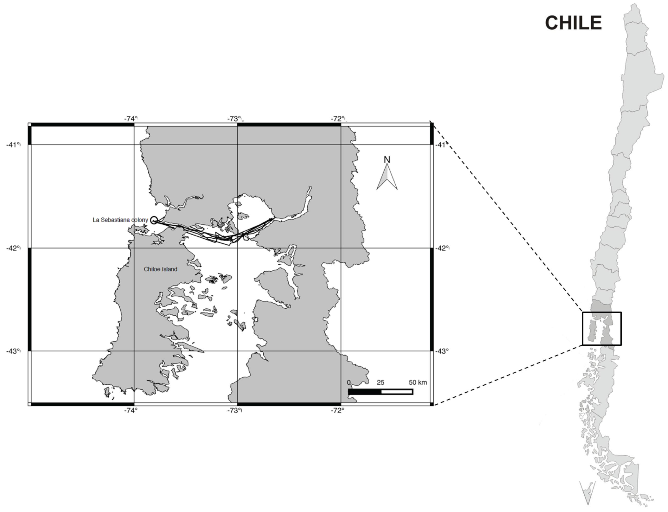
4.2. Real Data
5. Conclusions
Acknowledgments
Author Contributions
Conflicts of Interest
References
- Harrison, J.M.; Shepp, L.A. On Skew Brownian motion. Ann. Probab. 1981, 9, 309–313. [Google Scholar] [CrossRef]
- Lejay, A. On the constructions of the Skew Brownian motion. Probab. Surv. 2006, 3, 413–466. [Google Scholar]
- Kutoyants, Y. Parameter Estimation for Stochastic Processes; Heldermann: Berlin, Germany, 1984. [Google Scholar]
- Lipster, R.; Shiryaev, A. Statistics of Random Processes II, Applications; Springer: Berlin/Heidelberg, Germany, 2001. [Google Scholar]
- Florens-Zmirou, D. Statistics on crossings of discretized diffusions and local time. Stoch. Process. Appl. 1993, 39, 139–151. [Google Scholar] [CrossRef]
- Jacod, J. Rates of convergence to the local time of a diffusion. Annales de l’IHP Probabilités et statistiques 1998, 34, 505–544. [Google Scholar] [CrossRef]
- Bardou, O.; Martinez, M. Statistical estimation for reflected skew processes. Stat. Inference Stoch. Process. 2010, 13, 231–248. [Google Scholar] [CrossRef]
- Lejay, A.; Mordecki, E.; Torres, S. Is the Brownian motion skew? Scand. J. Stat. 2014, 41, 346–364. [Google Scholar] [CrossRef]
- Boness, D.J.; Bowen, W.D.; Oftedall, O.T. Evidence of a maternal foraging cycle resembling that of otariid seals in a small phocid, the harbor seal. Behav. Ecol. Sociobiol. 1994, 34, 95–104. [Google Scholar] [CrossRef]
- Karatzas, I.; Shreve, S. Brownian Motion and Stochastic Calculus; Springer: Berlin/Heidelberg, Germany, 1991. [Google Scholar]
- Walsh, J.B. A diffusion with a discontinuous local time. Astérisque 1978, 52, 37–45. [Google Scholar]
- Breiman, L. Probability; SIAM: Philadelphia, PA, USA, 1992. [Google Scholar]
- Pereira, C.A.B.; Stern, J.M.; Wechsler, S. Can a significance test be genuinely bayesian? Bayesian Anal. 2008, 3, 15–36. [Google Scholar] [CrossRef]
- Rifo, L.; González-López, V. Full Bayesian analysis for a model of tail dependence. Commun. Stat. Theory Methods 2012, 41, 4107–4123. [Google Scholar] [CrossRef]
- Madruga, M.R.; Esteves, L.G.; Wechsler, S. On the bayesianity of Pereira–Stern tests. Test 2001, 10, 291–299. [Google Scholar] [CrossRef]
- Verdinelli, I.; Wasserman, L. Computing bayes factors using a generalization of the savage-dickey density ratio. J. Am. Stat. Assoc. 1995, 90, 614–618. [Google Scholar] [CrossRef]
- Bonadonna, F.; Lea, M.-A.; Dehorter, O.; Guinet, C. Foraging ground fidelity and route-choice tactics of a marine predator: The Antarctic fur seal Arctocephalus gazella. Mar. Ecol. Prog. Ser. 2001, 223, 277–286. [Google Scholar] [CrossRef]
- Robson, B.W.; Goebel, M.E.; Baker, J.D.; Ream, R.R.; Loughlin, T.R.; Francis, R.C.; Antonelis, G.A.; Costa, D.P. Separation of foraging habitat among breeding sites of a colonial marine predator, the northern fur seal (Callorhinus ursinus). Can. J. Zool. 2004, 82, 20–29. [Google Scholar] [CrossRef]
- Call, K.A.; Ream, R.R.; Johnson, D.; Sterling, J.T.; Towell, R.G. Foraging route tactics and site fidelity of adult female northern fur seal (Callorhinus ursinus) around the Pribilof Islands. Deep Sea Res. II 2008, 55, 1883–1896. [Google Scholar] [CrossRef]
- Riet-Sapriza, F.G.; Costa, D.P.; Franco-Trecu, V.; Marín, Y.; Chocca, J.; González, B.; Beathyate, G.; Chilvers, B.L.; Hückstadt, L.A. Foraging behavior of lactating South American sea lions (Otaria flavescens) and spatial-temporal resource overlap with the Uruguayan fisheries. Deep Sea Res. II 2013, 88–89, 106–119. [Google Scholar] [CrossRef]
- Rodríguez, D.H.; Dassis, M.; de León, A.P.; Barreiro, C.; Farenga, M.; Bastida, R.O.; Davis, R.W. Foraging strategies of Southern sea lion females in the La Plata River Estuary (Argentina-Uruguay). Deep Sea Res. II 2013, 88–89, 120–130. [Google Scholar] [CrossRef]
- Friedlaender, A.S.; Halpin, P.N.; Qian, S.S.; Lawson, G.L.; Wiebe, P.H.; Thiele, D.; Read, A.J. Whale distribution in relation to prey abundance and oceanographic processes in shelf waters of the Western Antarctic Peninsula. Mar. Ecol. Prog. Ser. 2006, 317, 297–310. [Google Scholar] [CrossRef]
- Leung, E.S.; Chilvers, B.L.; Nakagawa, S.; Moore, A.B.; Robertson, B.C. Sexual segregation in juvenile New Zealand sea lion foraging ranges: Implications for intraspecific competition, population dynamics and conservation. PLoS ONE 2012, 7, e45389. [Google Scholar] [CrossRef] [PubMed]
- Cappozzo, H.L.; Perrin, W.F. South American sea lion (Otaria flavescens). In Encyclopedia of Marine Mammals; Elsevier: Amsterdam, The Netherlands, 2008; pp. 1076–1079. [Google Scholar]
- Sigler, M.F.; Tollit, D.J.; Vollenweider, J.J.; Thedinga, J.F.; Csepp, D.J.; Womble, J.N.; Wong, M.A.; Rehberg, M.J.; Trites, A.W. Steller sea lion foraging response to seasonal changes in prey availability. Mar. Ecol. Prog. Ser. 2009, 388, 243–261. [Google Scholar] [CrossRef]


| Prior Distribution | Posterior Mode | Posterior Mean | e-Value | Bayes Factor |
|---|---|---|---|---|
| for θ | for | for | for | against |
| Beta(1,1) | ||||
| Beta(1,5) |
| Prior Distribution | Posterior Mode | Posterior Mean | e-Value | Bayes Factor | |
|---|---|---|---|---|---|
| for θ | for | for | for | against | |
| Beta(1,1) | |||||
| Beta(5,1) | |||||
| Beta(1,5) |
© 2016 by the authors; licensee MDPI, Basel, Switzerland. This article is an open access article distributed under the terms and conditions of the Creative Commons Attribution (CC-BY) license (http://creativecommons.org/licenses/by/4.0/).
Share and Cite
Barahona, M.; Rifo, L.; Sepúlveda, M.; Torres, S. A Simulation-Based Study on Bayesian Estimators for the Skew Brownian Motion. Entropy 2016, 18, 241. https://doi.org/10.3390/e18070241
Barahona M, Rifo L, Sepúlveda M, Torres S. A Simulation-Based Study on Bayesian Estimators for the Skew Brownian Motion. Entropy. 2016; 18(7):241. https://doi.org/10.3390/e18070241
Chicago/Turabian StyleBarahona, Manuel, Laura Rifo, Maritza Sepúlveda, and Soledad Torres. 2016. "A Simulation-Based Study on Bayesian Estimators for the Skew Brownian Motion" Entropy 18, no. 7: 241. https://doi.org/10.3390/e18070241
APA StyleBarahona, M., Rifo, L., Sepúlveda, M., & Torres, S. (2016). A Simulation-Based Study on Bayesian Estimators for the Skew Brownian Motion. Entropy, 18(7), 241. https://doi.org/10.3390/e18070241