Sparse Estimation Based on a New Random Regularized Matching Pursuit Generalized Approximate Message Passing Algorithm

Abstract

Approximate Message Passing (AMP) and Generalized AMP (GAMP) algorithms usually suffer from serious convergence issues when the elements of the sensing matrix do not exactly match the zero-mean Gaussian assumption. To stabilize AMP/GAMP in these contexts, we have proposed a new sparse reconstruction algorithm, termed the Random regularized Matching pursuit GAMP (RrMpGAMP). It utilizes a random splitting support operation and some dropout/replacement support operations to make the matching pursuit steps regularized and uses a new GAMP-like algorithm to estimate the non-zero elements in a sparse vector. Moreover, our proposed algorithm can save much memory, be equipped with a comparable computational complexity as GAMP and support parallel computing in some steps. We have analyzed the convergence of this GAMP-like algorithm by the replica method and provided the convergence conditions of it. The analysis also gives an explanation about the broader variance range of the elements of the sensing matrix for this GAMP-like algorithm. Experiments using simulation data and real-world synthetic aperture radar tomography (TomoSAR) data show that our method provides the expected performance for scenarios where AMP/GAMP diverges.

1. Introduction

Compressed Sensing (CS) has been a research focus in recent years. The idea of sparse estimation and compressed sensing has also been applied in adaptive filtering [1,2,3,4] and nonlinear dynamics systems [5,6]. Define the support of an unknown K-sparse $(K\ll N)$ vector $\mathbf{x}\in {\mathbb{C}}^N$ as: $S=\{j:j\in \{1,\cdots ,N\},x_j\ne 0\}$. We consider an under-determined noisy linear system:

$$\mathbf{y}=\mathbf{A}\mathbf{x}+\mathit{ϵ}$$

(1)

where $\mathbf{y}\in {\mathbb{C}}^M$ is the measurement vector, $\mathit{ϵ}\in {\mathbb{C}}^M$ is the additive Gaussian noise vector and $\mathbf{A}\in {\mathbb{C}}^{M\times N}$ $(M<N)$ is the projection matrix, also termed the sensing matrix. The aim of CS is to reconstruct $\mathbf{x}$ from $\mathbf{y}$ and $\mathbf{A}$.

On the one hand, it is well known that the CS problem can be rephrased into a probabilistic inference problem on the bipart factor graph shown in Figure 1a. Donoho et al. proposed the Approximate Message Passing (AMP) algorithm [7,8] to solve it. Rangan et al. generalized AMP to adapt to an arbitrary sparse prior and arbitrary measurement noise; their work is called the Generalized Approximate Message Passing (GAMP) algorithm [9]. Since the derivation of AMP/GAMP is based on a zero-mean Gaussian projection matrix hypothesis, they cannot work well if the projection matrix does not satisfy the hypothesis, as shown in Section 4. This phenomenon motivates us to improve the AMP/GAMP algorithm for a more general projection matrix. On the other hand, although ${\ell }_0$ methods, such as Orthogonal Matching Pursuit (OMP) [10] and Compressive Sampling Matching Pursuit (CoSaMP) [11], are simple and effective, they use Least Squares (LS) to calculate the amplitude of non-zero elements. Therefore, these methods have to face the matrix inversion problem. When the scale of the projection matrix is small, this problem is not serious. However, when the scale becomes larger, the multipliers grow cubically as a function of sparsity K. This drawback stimulates us to find some approach to replace the LS step in ${\ell }_0$ methods and to overcome the disadvantages of OMP and CoSaMP.

In this paper, we propose a new sparse estimation algorithm, termed Random regularized Matching pursuit Generalized Approximate Message Passing (RrMpGAMP), to solve the CS problem. Our method can be regarded as a kind of ${\ell }_0$ optimization algorithm, termed Random regularized Matching Pursuit (RrMP), but the mean and variance estimation of x are the output of a restricted GAMP algorithm, termed the Fixed support GAMP (FsGAMP). In this way, it allows a more general projection matrix and does not calculate the inverse matrix directly. The computational complexity of RrMpGAMP is comparable to GAMP, and the memory occupation of RrMpGAMP is much less than GAMP and other LS-based algorithms.

The rest of this paper is organized as follows. We describe the RrMpGAMP algorithm in Section 2, then analyze the convergence of FsGAMP by the replica method in Section 3 and then perform experiments in Section 4. We draw a conclusion in the last Section 5. The derivation of the FsGAMP algorithm is provided in the Appendix.

2. Random Regularized Matching Pursuit Generalized Approximate Message Passing

As mentioned in the Introduction, the RrMpGAMP algorithm includes two parts: the RrMP algorithm and the FsGAMP algorithm, which is embedded in RrMP. The former is a new ${\ell }_0$ optimization algorithm; the latter is a tiny revised GAMP algorithm.

At the beginning, we assume the support S has been known, which means the probability of every zero element in $\mathbf{x}$ is one. Therefore, we just need to consider the probability of other non-zero elements in $\mathbf{x}$. We suppose that the Probability Distribution Function (PDF) of $\mathbf{x}$ and the likelihood function of $\mathbf{z}=\mathbf{Ax}$ are separable, i.e.,

$$\begin{array}{cc}\hfill p_{\mathit{x}}(\mathbf{x})& =1\times p_{{\mathit{x}}_S}({\mathbf{x}}_S)={\prod }_{j=1}^K{p}_{{\mathsf{x}}_{S_j}}(x_{S_j})\hfill \end{array}$$

(2)

$$\begin{array}{cc}\hfill p_{\mathit{y}|\mathit{z}}(\mathbf{y}|\mathbf{z})& ={\prod }_{m=1}^M{p}_{{\mathsf{y}}_m|{\mathsf{z}}_m}(y_m|z_m)\hfill \end{array}$$

(3)

Therefore, the probabilistic form of Equation (1) can be written as:

$$\begin{array}{cc}\hfill p_{\mathit{x}|\mathit{y}}(\mathbf{x}|\mathbf{y})& =1\times p_{{\mathit{x}}_S|\mathit{y}}({\mathbf{x}}_S|\mathbf{y})\propto p_{\mathit{y}|{\mathit{x}}_S}(\mathbf{y}|{\mathbf{x}}_S)p_{{\mathit{x}}_S}({\mathbf{x}}_S)\hfill \\ & ={\prod }_{m=1}^M{p}_{{\mathsf{y}}_m|{\mathsf{z}}_m}\left(y_m|a_{m{S}_k}{x}_{S_k}+{\sum }_{j\ne k}^K{a}_{m{S}_j}{x}_{S_j}\right){\prod }_{j=1}^K{p}_{{\mathsf{x}}_{S_j}}(x_{S_j})\hfill \end{array}$$

(4)

Actually we do not know S in the first place; a straightforward idea is to find it by some matching pursuit-based method.

2.1. Random Regularized Matching Pursuit Algorithm

A traditional matching pursuit algorithm (MP or OMP) finds an index of the non-zero element of $\mathbf{x}$ at each iteration. It does not rollback even if an incorrect index has been chosen. Our proposed algorithm sequentially pursues multiple indexes at each iteration and has the ability to undo, like the well-known Regularized OMP (ROMP) algorithm and the CoSaMP algorithm.

We use the subscript l to denote left, r to denote right and $|U|$ to designate the cardinality of temporary support U. Define three functions appearing in the algorithm: $\mathtt{FixSuppGAMP}(\mathbf{y},\mathbf{A},U)$ calculates the mean and variance estimation of $\mathbf{x}$; $R_{2s\backslash s}(\mathbf{v})$ finds the indexes of the $2s<K$ absolutely largest entries of $\mathbf{v}$, where s is the probe length, and then shuffles these indexes and bisects them; the outputs are the left and right indexes’ subset and the amplitudes supported on them, respectively; support updating function $H(\mathbf{u},\mathbf{c},\mathsf{\Lambda },S)$ generates a new indexes’ set by a group of rules; we will explain it soon.

The steps of RrMP are listed in Algorithm 1.

Algorithm 1 Random Regularized Matching Pursuit.
Input: $\mathbf{y},\mathbf{A},K,s$
Output: ${\mathbf{x}}^{n+1}$
1:	$S^0\leftarrow \varnothing ,{\mathbf{x}}^0\leftarrow \mathbf{0}$
2:	$({\mathsf{\Lambda }}_l,{\mathbf{c}}_l,{\mathsf{\Lambda }}_r,{\mathbf{c}}_r)\leftarrow R_{2s\backslash s}({\mathbf{A}}^T(\mathbf{y}-\mathbf{A}{\mathbf{x}}^n))$
3:	$U_l\leftarrow S^n\cup {\mathsf{\Lambda }}_l$, $U_r\leftarrow S^n\cup {\mathsf{\Lambda }}_r$
4:	${\mathbf{u}}_l\leftarrow \mathtt{FixSuppGAMP}(\mathbf{y},\mathbf{A},U_l)$
5:	${\mathbf{u}}_r\leftarrow \mathtt{FixSuppGAMP}(\mathbf{y},\mathbf{A},U_r)$
6:	$\theta ={arg\; min}_{\{l,r\}}\{\parallel \mathbf{y}-\mathbf{A}{\mathbf{u}}_l{\parallel }_2,\parallel \mathbf{y}-\mathbf{A}{\mathbf{u}}_r{\parallel }_2\}$
7:	${\mathsf{\Lambda }}^{n+1}\leftarrow {\mathsf{\Lambda }}_{\theta },{\mathbf{c}}^{n+1}\leftarrow {\mathbf{c}}_{\theta },{\mathbf{u}}^{n+1}\leftarrow {\mathbf{u}}_{\theta },U^{n+1}\leftarrow U_{\theta }$
8:	$S^{n+1}\leftarrow H({\mathbf{u}}^{n+1},{\mathbf{c}}^{n+1},{\mathsf{\Lambda }}^{n+1},S^n)$
9:	${\mathbf{x}}^{n+1}\leftarrow \mathtt{FixSuppGAMP}(\mathbf{y},\mathbf{A},S^{n+1})$

They are separated into two stages: the first stage is Lines 2–5, and the second stage is Lines 6–9. At the first stage, Line 2 obtains two index candidates, ${\mathsf{\Lambda }}_l$ and ${\mathsf{\Lambda }}_r$, and the correlation coefficients between the residual and columns of $\mathbf{A}$, ${\mathbf{c}}_l$ and ${\mathbf{c}}_r$. It is a key step, since the shuffle and bisecting operations are equivalent to a random search in N dimensional $\{0,1\}$ space. Line 3 merges the previous support set $S^n$ with two current candidates, respectively. Lines 4 and 5 roughly estimate $\mathbf{x}$ by the FsGAMP algorithm. At this stage, the candidate indexes are not replaced/dropped. Therefore, the number of possible incorrect indexes is typically greater than that at the second stage. This is the meaning of “roughly”. At the second stage, Lines 6 and 7 choose the minimal residual branch as a new candidate. This prune operation can be regarded as a regularization since the algorithm chooses a small residual branch and discards a big residual branch. In another words, the algorithm discards half of the candidate indexes pursued by Line 2. Line 8 updates the support set. Line 9 estimates $\mathbf{x}$ again. Note that Lines 3–5 can be calculated by parallel computing.

We define the precision τ as the ratio of the residual norm over the measurement norm, and set the error bound to $0.01$, which means $99.99\%$ of the measurement energy has been recovered. When $|P|$ equals sparsity K, if the precision does not reach the error bound, set $S^{n+1}=P$, keep running RrMP at most $2s$ times and then stop the algorithm.

The idea of the support updating function comes from two observations: (i) not all indexes in the candidate set are correct, so the algorithm should drop or replace a part of the indexes, as shown in Equations (7) and (8); the dropout/replacement operations can be regarded as a regularization; (ii) the candidate indexes corresponding to correlations ${\mathbf{c}}^{n+1}$ and to amplitudes ${\mathbf{u}}^{n+1}$ are not overlapping entirely; some correct indexes belong to the former, and some belong to the latter. It is necessary to merge them, as shown in Equation (9).

Now, we define the support updating function $H({\mathbf{u}}^{n+1},{\mathbf{c}}^{n+1},{\mathsf{\Lambda }}^{n+1},S^n)$ as follows. Firstly, define two threshold functions corresponding to the sparse representation coefficients $\mathbf{u}$, which are evolved with iterations:

$$\begin{array}{cc}\hfill a& \triangleq \underset{i\in S^n}{min}\{{|({\mathbf{u}}^{n+1})|}_i\}\hfill \end{array}$$

(5)

$$\begin{array}{cc}\hfill b& \triangleq \underset{j\in {\mathsf{\Lambda }}^{n+1}}{max}\{{|({\mathbf{u}}^{n+1})|}_j\}\hfill \end{array}$$

(6)

Secondly, define the indexes’ updating procedure just for $\mathbf{u}$:

$$P\triangleq \left\{\begin{array}{cc}{S}^n\cup \{j:{arg\; max}_{j\in {\mathsf{\Lambda }}^{n+1}}\{|{({\mathbf{u}}^{n+1})}_j|\}\},\hfill & \frac{a}{2}>b\hfill \\ S^n\cup \{j:j\in {\mathsf{\Lambda }}^{n+1},|{({\mathbf{u}}^{n+1})}_j|\ge \frac{a}{2}\},\hfill & a>b\ge \frac{a}{2}\hfill \\ S^n\cup \{j:j\in {\mathsf{\Lambda }}^{n+1},|{({\mathbf{u}}^{n+1})}_j|\ge \frac{b}{2}\},\hfill & b>a\ge \frac{b}{2}\hfill \\ \left\{i:i\in S^n,|{({\mathbf{u}}^{n+1})}_i|\ge \frac{b}{2}\right\}\cup \left\{j\in {\mathsf{\Lambda }}^{n+1},|{({\mathbf{u}}^{n+1})}_j|\ge \frac{b}{2}\right\},\hfill & \frac{b}{2}\ge a\hfill \end{array}\right.$$

(7)

Thirdly, define the the indexes’ updating procedure just for the correlation coefficients $\mathbf{c}$:

$$Q\triangleq \{j:j\in {\mathsf{\Lambda }}^{n+1},|{({\mathbf{c}}^{n+1})}_j|\ge 0.5\parallel {\mathbf{c}}^{n+1}{\parallel }_{\infty }\}$$

(8)

Lastly, we merge the two index sets to obtain the output of:

$$S^{n+1}=P\cup Q$$

(9)

These update rules are inspired by the regularized OMP algorithm [12,13]. It seems a bit complex, but the basic rationale is simple. We segment the absolute amplitudes on the pursued support at each iteration to ladders; the height of each ladder is dominated by the minimum of the absolute amplitudes, which is supported on the previous pursued support set $S^n$, and by the maximum of absolute amplitudes, which is supported on the current candidate support set ${\mathsf{\Lambda }}^{n+1}$. Since the square of the amplitude is energy, the absolute amplitudes in the same ladder step can be explained to obey a similar energy level. For Equation (7),

• If $\frac{a}{2}>b$, this means that the absolute amplitudes of the current candidate indexes are much smaller than the absolute amplitudes of the previous pursued indexes, so the algorithm chooses only one current candidate index. This situation corresponds to a sharp ladder step.
• If $a>b\ge \frac{a}{2}$, this means the absolute amplitudes of the current candidate indexes are just a little smaller than the absolute amplitudes of the previous pursued indexes, so the algorithm chooses those indexes whose absolute amplitudes are greater than $a/2$. This situation corresponds to a flattened ladder step.
• If $b>a\ge \frac{b}{2}$, this means the absolute amplitudes of the current candidate indexes are greater than the absolute amplitudes of the previous pursued indexes, but the minimum absolute amplitude of the previous pursued indexes is not a very small value, so the algorithm chooses those indexes whose absolute amplitudes are greater than $b/2$. This situation also corresponds to a flattened ladder step.
• If $\frac{b}{2}>a$, that means the minimum absolute amplitude of the previous pursued indexes is very small, so the algorithm drops a part of the previous pursued indexes and adds a part of the current candidate indexes. This situation corresponds to a sharp ladder step.

However, it is not enough to choose indexes just by absolute amplitudes. Some correlations about the residual and the columns of $\mathbf{A}$ are significant. The algorithm finds these indexes by Line 2 in Algorithm 1. Maybe, the absolute amplitudes supporting them are not significant, such that they are excluded by Equation (7). We can imagine these indexes as free electrons that are escaping to other energy levels. Therefore, the algorithm should retrieve them. This is the meaning of Equation (8). The rules are heuristic, the explanations are analogies to physics.

2.2. Fixed Support GAMP Algorithm

The concept of message passing on a factor graph can be found in [14]. In contrast to AMP/GAMP, the FsGAMP algorithm does not reform Equation (1) to a bipart graph. It restricts the edges to a part of variable nodes, which correspond to the temporary support U, as shown in Figure 1b. Based on this factor graph and the posterior probability Equation (4), firstly, we define the messages from the factor node to the variable node. For the Max-Sum rule, they are:

$$\begin{array}{cc}\hfill {\mathbf{\Delta }}_{{\mathsf{f}}_m\to {\mathsf{x}}_{U_k}}(t,x_{U_k})& \triangleq \underset{\begin{array}{c}{\mathbf{x}}_U\end{array}}{max}[log{p}_{{\mathsf{y}}_m|{\mathsf{z}}_m}\left(y_m|a_{m{U}_k}{x}_{U_k}+{\sum }_{j\ne k}^{|U|}{a}_{m{U}_j}{x}_{U_j}\right)\hfill \\ \mathrm{(10)}& & +{\sum }_{j\ne k}^{|U|}{\mathbf{\Delta }}_{{\mathsf{f}}_m\leftarrow {\mathsf{x}}_{U_j}}(t,x_{U_j})]+\mathsf{c}\hfill \end{array}$$

where $\mathsf{c}$ means constant ; for the Sum-Product rule, they are:

$$\begin{array}{cc}\hfill {\mathbf{\Delta }}_{{\mathsf{f}}_m\to {\mathsf{x}}_{U_k}}(t,x_{U_k})& \triangleq log[{\int }_{{\{x_{U_j}\}}_{j\ne k}}{p}_{{\mathsf{y}}_m|{\mathsf{z}}_m}\left(y_m|a_{m{U}_k}{x}_{U_k}+{\sum }_{j\ne k}^{|U|}{a}_{m{U}_j}{x}_{U_j}\right)\hfill \\ \mathrm{(11)}& & \times {\prod }_{j\ne k}^{|U|}exp\left({\mathbf{\Delta }}_{{\mathsf{f}}_m\leftarrow {\mathsf{x}}_{U_j}}(t,x_{U_j})\right)]+\mathsf{c}\hfill \end{array}$$

Secondly, we define the messages from the variable node to the factor node. The form of the Max-Sum rule is the same as the form of the Sum-Product rule:

$${\mathbf{\Delta }}_{{\mathsf{f}}_m\leftarrow {\mathsf{x}}_{U_k}}(t+1,x_{U_k})\triangleq log{p}_{{\mathsf{x}}_{U_k}}(x_{U_k})+{\sum }_{i\ne m}^M{\mathbf{\Delta }}_{{\mathsf{f}}_i\to {\mathsf{x}}_{U_k}}(t,x_{U_k})+\mathsf{c}$$

(12)

The derivation of FsGAMP is very similar with GAMP [9]. Due to space limitations, we only emphasize the difference in the main body and left the details to the Appendix. Since $|U|$ non-zero elements of $\mathbf{x}$ have been pursued, we set other elements of $\mathbf{x}$ to zero directly, such that the ${\sum }_{j\ne k}^N{a}_{mj}{x}_j$ and ${\sum }_{j\ne k}^N{|a_{mj}|}^2{x}_j$ terms in GAMP reduce to ${\sum }_{j\ne k}^{|U|}{a}_{m{U}_j}{x}_{U_j}$ and ${\sum }_{j\ne k}^{|U|}{|a_{m{U}_j}|}^2{x}_{U_j}$. Other derivation steps are the same as GAMP. It is worth noting that the derivation of GAMP is primarily based on the Central-Limit Theorem (CLT), but in FsGAMP, this condition is canceled, because we have known the index set of zero elements (though maybe incorrect), such that the mean and variance estimation of these elements are also zeros. This simplification eliminates uncertainty and brings stability to FsGAMP to adapt more types of projection matrices.

Rangan et al. [9,15] investigated the influence of damping in GAMP. They found that damping can induce convergence. Similar steps are used in the FsGAMP algorithm:

$$\begin{array}{cc}\hfill {\nu }^{\mathbf{p}}(t)& =\delta {\nu }^{\mathbf{p}}(t)+(1-\delta ){\nu }^{\mathbf{p}}(t-1)\hfill \end{array}$$

(13)

$$\begin{array}{cc}\hfill \widehat{\mathbf{s}}(t)& =\delta \widehat{\mathbf{s}}(t)+(1-\delta )\widehat{\mathbf{s}}(t-1)\hfill \end{array}$$

(14)

$$\begin{array}{cc}\hfill {\nu }^{\mathbf{s}}(t)& =\delta {\nu }^{\mathbf{s}}(t)+(1-\delta ){\nu }^{\mathbf{s}}(t-1)\hfill \end{array}$$

(15)

$$\begin{array}{cc}\hfill \widehat{\mathbf{x}}(t)& =\delta \widehat{\mathbf{x}}(t)+(1-\delta )\widehat{\mathbf{x}}(t-1)\hfill \end{array}$$

(16)

The steps of FsGAMP are listed in Algorithm 2. Notation t indicates the iteration number; $\widehat{\mathbf{x}}$ and ${\nu }^{\mathbf{x}}$ denote the mean and variance of $\mathbf{x}$; the element-wise product and division are denoted ⊙ and ⊘. Function $g_{\text{out}}(·)$ and $g_{\text{in}}(·)$ calculate the Bayesian estimation of $\mathbf{z}$ and $\mathbf{x}$, respectively. Please refer to [9] (Table 1) and the Appendix to find their specific forms. The prior $p_{\mathsf{x}}(x_{S_j})$ can take a Gaussian, Laplacian or spike-and-slab distribution.

Algorithm 2 Fix Support GAMP.
Input: $\mathbf{y};\mathbf{A};U$
Output: $\widehat{\mathbf{x}};{\nu }^{\mathbf{x}}$
1:	$\widehat{\mathbf{x}}\leftarrow {\mathbf{0}}^{N\times 1};{\nu }^{\mathbf{x}}\leftarrow {\mathbf{0}}^{N\times 1};\widehat{\mathbf{s}}(t=0)\leftarrow {\mathbf{0}}^{M\times 1}$
2:	${\widehat{\mathbf{x}}}_U(t=1)\leftarrow {\mathbf{0}}^{|U|\times 1};{\nu }^{{\mathbf{x}}_U}(t=1)\leftarrow {\mathbf{0}}^{|U|\times 1}$
3:	while $stop=$ false do
4:	${\nu }^{\mathbf{p}}(t)\leftarrow {|{\mathbf{A}}_{:,U}|}^2{\nu }^{{\mathbf{x}}_U}(t)$
5:	$\widehat{\mathbf{z}}(t)\leftarrow {\mathbf{A}}_{:,U}{\widehat{\mathbf{x}}}_U(t)$
6:	$\widehat{\mathbf{p}}(t)\leftarrow \widehat{\mathbf{z}}(t)-\widehat{\mathbf{s}}(t-1)\odot {\nu }^{\mathbf{p}}(t)$
7:	$[{\widehat{\mathbf{z}}}_0(t),{\nu }^{{\mathbf{z}}_0}(t)]\leftarrow g_{\text{out}}(\widehat{\mathbf{p}}(t),{\nu }^{\mathbf{p}}(t))$
8:	$\widehat{\mathbf{s}}(t)\leftarrow (1\oslash {\nu }^{\mathbf{p}}(t))\odot ({\widehat{\mathbf{z}}}_0(t)-\widehat{\mathbf{p}}(t))$
9:	${\nu }^{\mathbf{s}}(t)\leftarrow (1\oslash {\nu }^{\mathbf{p}}(t))\odot (1-{\nu }^{{\mathbf{z}}_0(t)}\oslash {\nu }^{\mathbf{p}}(t))$
10:	${\nu }^{{\mathbf{r}}_U}(t)\leftarrow 1\oslash ({({|{\mathbf{A}}_{:,U}|}^2)}^T{\nu }^{\mathbf{s}}(t))$
11:	${\widehat{\mathbf{r}}}_U(t)\leftarrow {\widehat{\mathbf{x}}}_U(t)+{\nu }^{{\mathbf{r}}_U}(t)\odot ({\mathbf{A}}_{:,U}^T\widehat{\mathbf{s}}(t))$
12:	$[{\widehat{\mathbf{x}}}_U(t+1),{\nu }^{{\mathbf{x}}_U}(t+1)]\leftarrow g_{\text{in}}({\widehat{\mathbf{r}}}_U(t),{\nu }^{{\mathbf{r}}_U}(t))$
13:	{damping steps}
14:	if $\parallel {\widehat{\mathbf{x}}}_U(t+1)-{\widehat{\mathbf{x}}}_U{(t)\parallel }_2/{\parallel {\widehat{\mathbf{x}}}_U(t)\parallel }_2\le \delta$ then
15:	$\widehat{\mathbf{x}}(U)\leftarrow {\widehat{\mathbf{x}}}_U(t+1),{\nu }^{\mathbf{x}}(U)\leftarrow {\nu }^{{\mathbf{x}}_U}(t+1)$
16:	$stop\leftarrow$ TRUE
17:	end if
18:	end while

GAMP calculates all elements of $\mathbf{x}$ in the loop, while FsGAMP estimates at most $|U|$ non-zero elements of $\mathbf{x}$ in the loop. Since $|U|$ increases gradually and $|U|\le K$, the memory footprint rate of FsGAMP is not more than $K/N$. Because $K\ll N$, the memory saving is remarkable.

2.3. Computational Complexity Discussion

The computational complexity of the GAMP algorithm is dominated by four matrix-vector multipliers per iteration [9]. The multipliers of FsGAMP coincide with GAMP: Lines 4, 6, 10 and 11. At each multiplication, the FsGAMP algorithm only computes $M\times |S|$ multipliers, while the GAMP algorithm needs $M\times N$ multipliers.

RrMpGAMP has two nested loops; the outer loop is RrMP; the inner loops are three FsGAMPs. Because the replacement/dropout operations in the RrMP algorithm are random, we cannot exactly calculate how many new indexes are chosen per iteration. However, if we roughly estimate the number of winners in these candidates to $s/2$ per iteration (usually, this number is greater than $s/2$ with the step in observation), the outer loop has $J=\lceil K/(s/2)\rceil +2s$ iterations. Furthermore, $2s$ can be removed, since it is a small quantity compared to $\lceil K/(s/2)\rceil$. Because the number of iterations of GAMP (as well as FsGAMP) is also uncertain, we simply use the maximal iteration number B as the worst setting. Firstly, taking no account of M and B, we have:

$$\begin{array}{c}(2s+\frac{s}{2})+(2(\frac{s}{2}+s)+\frac{s}{2})+(2(\frac{2s}{2}+s)+\frac{3s}{2})+\cdots +(2(\frac{(J-1)s}{2}+s)+\frac{Js}{2})\hfill \\ \hfill =2[s+\frac{s}{2}+s+\frac{2s}{2}+s+\cdots +\frac{(J-1)s}{2}+s]+(\frac{s}{2}+\frac{2s}{2}+\frac{3s}{2}+\cdots +\frac{Js}{2})\end{array}$$

(17)

where the first square brackets correspond to Lines 4–5 in Algorithm 1, and the second square brackets correspond to Line 9 in Algorithm 1. After summation and simplification, we have:

$$Equation(17)=\frac{Js(3J+7)}{4}$$

(18)

Secondly, considering M, B, four matrix-vector multiplies per iteration, and expanding J, we have:

$$Equation(18)\Rightarrow O(4MB{J}^{2}s)=O(16MKB)$$

(19)

For GAMP, the computational complexity can be estimated as $O(4MNB)$, If $4K<N$, the computational complexity of RrMpGAMP is less than GAMP.

Using the matching pursuit-based methods to solve a M-row n-column linear system, the computing time mainly depends on the least squares step, especially when the number of equations M is large and the number of variables n is not small. For example, the Householder-LS method needs $O(2n^2(M-n/3))$ flops ([16], Algorithm 5.3.2). Because OMP finds one column index at a time and n increases from one to K, the computational complexity of OMP using Householder-LS is:

$$\begin{array}{cc}\hfill \sum _{n=1}^{K}O(2n^2(M-n/3))& =O\left(\sum _{n=1}^{K}2M{n}^2-\sum _{n=1}^K\frac{2}{3}{n}^3\right)\hfill \\ & =O\left(2M\frac{K(K+1)(2K+1)}{6}-\frac{2}{3}{(\frac{K(K+1)}{2})}^2\right)\hfill \\ \mathrm{(20)}& & =O(M{K}^3)\hfill \end{array}$$

since $K\ll M$. We compare two computational complexity results. For RrMpGAMP, it is $O(16MBK)$; for OMP using Householder-LS, it is $O(M{K}^3)$. If $16B<K^2$, the computational complexity of RrMpGAMP is less than Householder-LS OMP.

3. Convergence Discussion

We use the replica method [17,18] to asymptotically describe the evaluation of the logarithm of the partition function of the posterior distribution Equation (4). We concentrate on the Sum-Product FsGAMP algorithm in this discussion. The main advantage is that replica computations give a statistical physical meaning to the linear system. The replica method was used for compressed sensing in recent years [19,20,21,22]; we follow the research of [23].

We use the zero-mean Gaussian matrix assumption in the derivation of FsGAMP and replica analysis, because FsGAMP just works on the RrMP pursued support set, and the cardinality of it is much smaller than the cardinality of a sparse vector, i.e., $|S|\ll N$. We know that the brief propagation on the factor graph tends to diverge if there are many cycles on it [14]. When the number of cycles decreases, the brief propagation tends to converge. The factor graph form of compressed sensing is a bipart graph, and there are too many cycles on it. However, if we restrict the connections to the pursued variable nodes and sequentially construct the connections by some kind of pursuit strategy, such as RrMP pursuit, the number of cycles increases from zero to a relatively small integer, compared to the huge number of bipart connection cycles. These relatively small cycles and sequential pursuit method can be seen as a regularization to the non-zero-mean reality. This is our intuition.

3.1. The Replica Method Analysis of FsGAMP

The zero-mean Gaussian measurement noise is assumed an equivalent variance Δ for every entry of $\mathit{ϵ}$, and generally, $\mathsf{\Delta }\ne {\mathsf{\Delta }}_0$, where ${\mathsf{\Delta }}_0$ is the true noise variance. This assumption means that the noise variance (inside ${\nu }^{{\mathbf{z}}_0}(t)$ term), which is estimated by the FsGAMP algorithm, usually does not equal the true noise variance. The influence of their difference is shown in Equation (74). We rewrite the definition of the CS problem as follows:

$$y_{\mu }=\sum _{i=1}^N{A}_{\mu i}{s}_i+{ϵ}_{\mu }\mu =1,\cdots ,M$$

(21)

where $\mathbf{s}$ is the original signal, and we use the notation s to replace notation x in Equation (1) to avoid ambiguity in the following derivation and use μ to replace m in accordance with the replica computations’ convention. We denote $\alpha =M/N$ with the number of measurements per variable. In the asymptotic analysis, we are interested in the case of large system limitation $N\to \infty$, while keeping signal density $p_{{\mathsf{x}}^0}(x^0)$ and measurement rate α of order one, where we let $x^0=s$. It is also necessary to assume that the components of signal $\mathbf{s}$ and measurement $\mathbf{y}$ are also order one, such that we can consider the elements of sensing matrix $\mathbf{A}$ to be zero-mean. It is worth noting that the variance of the order of $\mathbf{A}$’s elements is $O(1/K)$, not $O(1/N)$, because we have pursued the indexes of non-zero elements. This makes it not necessary for the FsGAMP algorithm to summarize N entries in one row of $\mathbf{A}$. In this way, the variance range of $\mathbf{A}$’s elements enlarges.

Before the start of the computation, we briefly review the link between a Hamiltonian and linear system estimation problems (we know the form of compressed sensing is a linear system). The posterior distribution of a linear system in the Boltzmann form is:

$$\begin{array}{ccc}& p(\mathbf{x}|\mathbf{y},\mathit{\theta })\hfill & =\frac{\mathbf{1}}{Z(\mathit{\theta })}{e}^{-E(\mathbf{x}|\mathbf{y},\mathit{\theta })}\hfill \\ \mathrm{(22)}& \hfill \Rightarrow & E(\mathbf{x}|\mathbf{y},\mathit{\theta })=-log(p(\mathbf{x}|\mathit{\theta }))-log(p(\mathbf{y}|\mathbf{x},\mathit{\theta }))\hfill \end{array}$$

where $p(\mathbf{x}|\mathit{\theta })$ is the prior, $\mathit{\theta }$ are the model parameters, such as:

$$p(\mathbf{x}|\mathit{\theta })=\prod _{i=1}^N\left[(1-\rho )\delta (x_i)+\rho \mathbf{N}(x_i|\tilde{\mathit{\theta }})\right]$$

(23)

Additionally, $p(\mathbf{y}|\mathbf{x},\mathit{\theta })$ is likelihood:

$$p(\mathbf{y}|\mathbf{x},\mathit{\theta })=\prod _{\mu =1}^M\mathcal{N}(y_{\mu }|{(\mathbf{Ax})}_{\mu },\mathit{\theta })$$

(24)

Then, we get the Hamiltonian:

$$E(\mathbf{x}|\mathbf{y},\mathit{\theta })=-\sum _{i=1}^{N}log(p_i(x_i))+\frac{1}{\mathsf{\Delta }}\sum _{\mu =1}^M{(y_{\mu }-{(\mathbf{Ax})}_{\mu })}^2+\frac{M}{2}log(2\pi \mathsf{\Delta })$$

(25)

Now, we derive the potential of Equation (21) under the pursued $|S|$ column indexes’ condition, as shown in Equation (4). The meaning of “potential” in inference theory equals the meaning of “Bethe free entropy” in statistical physics. For the simplification of notation, we ignore the uppercase letter S and just use the subscript, such as i, to indicate $S_i$ in Equation (4). The aim is to sample a vector $\mathbf{x}$ from the probability measure:

$$\begin{array}{cc}& p_{\mathit{x}|\mathit{y}}(\mathbf{x}|\mathbf{y})\hfill \\ \hfill =& \frac{1}{Z}\prod _{i=1}^K{p}_{{\mathsf{x}}_i}(x_i)\prod _{\mu =1}^M\frac{1}{\sqrt{2\pi \mathsf{\Delta }}}{e}^{-\frac{{[y_{\mu }-{\sum }_{i=1}^K{A}_{\mu i}{x}_i]}^2}{2\mathsf{\Delta }}}\hfill \\ \hfill =& \frac{1}{Z}\prod _{i=1}^K{p}_{{\mathsf{x}}_i}(x_{)}\prod _{\mu =1}^M\frac{1}{\sqrt{2\pi \mathsf{\Delta }}}{e}^{-\frac{{[{\sum }_{i=1}^K{A}_{\mu i}(x_i-s_i)+{ϵ}_{\mu }]}^2}{2\mathsf{\Delta }}}\hfill \end{array}$$

Equation (26) can be seen as the Boltzmann measure on a disordered system with Hamiltonian:

$$H(\mathbf{x})=-\sum _{i=1}^{K}log[p_{{\mathsf{x}}_i}(x_i)]+\frac{{[{\sum }_{i=1}^K{A}_{\mu i}(x_i-s_i)+{ϵ}_{\mu }]}^2}{2\mathsf{\Delta }}$$

(27)

where the partition function Z is the normalization constant of the full posterior distribution Equation (26) and $\mathbf{x}$ is the configuration of the Hamiltonian. The thermodynamic properties of the disordered system are characterized by the average free entropy ${\mathbb{E}}_{\mathbf{A},\mathbf{s},\mathit{ϵ}}(logZ)$, where:

$$Z(\mathbf{A},\mathbf{s},\mathit{ϵ})=\int \left[\prod _{i=1}^K\mathrm{d}{x}_i\prod _{i=1}^K{p}_{{\mathsf{x}}_i}(x_i)\right]\prod _{\mu =1}^M\frac{1}{\sqrt{2\pi \mathsf{\Delta }}}{e}^{-\frac{{[{\sum }_{i=1}^K{A}_{\mu i}(x_i-s_i)+{ϵ}_{\mu }]}^2}{2\mathsf{\Delta }}}$$

(28)

Because the expectation of the logarithm function is a hard problem, the average free entropy (also called the Bethe free entropy) can be evaluated via the replica trick as:

$$\mathsf{\Phi }\equiv \underset{K\to \infty }{lim}\frac{1}{K}{\mathbb{E}}_{\mathbf{A},\mathbf{s},\mathit{ϵ}}\{logZ\}=\underset{K\to \infty }{lim}\frac{1}{K}\underset{n\to 0}{lim}\frac{{\mathbb{E}}_{\mathbf{A},\mathbf{s},\mathit{ϵ}}\{Z^n\}-1}{n}$$

(29)

where n independent replicas are introduced to reform the original disordered system to a new system (i.e., the name of the method) and ${\mathbb{E}}_{\mathbf{A},\mathbf{s},\mathit{ϵ}}$ is the average over all of the sources of disorder in Equation (21). Each configuration of the new system is indexed by an n-tuple $\mathit{i}=(i_1,\cdots ,i_n)$, where each $i_a,a=1,\cdots ,n$ has a continuous non-zero state value because $i_a$ corresponds to a non-zero element in $\mathbf{x}$, which has been found by the matching pursuit process of the RrMP algorithm.

Now, the problem of computing the free energy is converted into computing the n-th moment of the partition function Z.

$${[Z(\mathbf{A},\mathbf{s},\mathit{ϵ})]}^n=\frac{1}{{(2\pi \mathsf{\Delta })}^{\frac{Mn}{2}}}\int \left[\prod _{i,a}\mathrm{d}{x}_i^a\prod _{i,a}{p}_{{\mathsf{x}}_i^a}(x_i^a)\right]\prod _{\mu }{e}^{-\frac{{\sum }_{a=1}^n{[{\sum }_{i=1}^K{A}_{\mu i}{s}_i+{ϵ}_{\mu }-{\sum }_{i=1}^K{A}_{\mu i}{x}_i^a]}^2}{2\mathsf{\Delta }}}$$

(30)

The average replicated partition function can be rearranged as:

$${\mathbb{E}}_{\mathbf{A},\mathbf{s},\mathit{ϵ}}\{Z^n\}=\frac{1}{{(2\pi \mathsf{\Delta })}^{\frac{Mn}{2}}}\int \left[\prod _{i,a}\mathrm{d}{x}_i^a\prod _{i,a}{p}_{{\mathsf{x}}_i^a}(x_i^a)\right]\prod _{\mu }{\mathbb{E}}_{\mathbf{A},\mathbf{s},\mathit{ϵ}}\left\{e^{-\frac{{\sum }_{a=1}^n{[{\sum }_{i=1}^K{A}_{\mu i}{s}_i+{ϵ}_{\mu }-{\sum }_{i=1}^K{A}_{\mu i}{x}_i^a]}^2}{2\mathsf{\Delta }}}\right\}$$

(31)

where $a,b,\cdots ,n$ denote the replica indexes. Define:

$$X_{\mu }={\mathbb{E}}_{\mathbf{A},\mathit{ϵ}}\left\{e^{-\frac{{\sum }_{a=1}^n{[{\sum }_{i=1}^K{A}_{\mu i}{s}_i+{ϵ}_{\mu }-{\sum }_{i=1}^K{A}_{\mu i}{x}_i^a]}^2}{2\mathsf{\Delta }}}\right\}$$

(32)

Equation (31) can be rewritten to:

$${\mathbb{E}}_{\mathbf{A},\mathbf{s},\mathit{ϵ}}\{Z^n\}=\frac{1}{{(2\pi \mathsf{\Delta })}^{\frac{Mn}{2}}}{\mathbb{E}}_{\mathbf{s}}\left\{\int \left[\prod _{i,a}\mathrm{d}{x}_i^a\prod _{i,a}{p}_{{\mathsf{x}}_i^a}(x_i^a)\right]\prod _{\mu =1}^M{X}_{\mu }\right\}$$

(33)

In order to compute $X_{\mu }$, firstly, we should define a variable:

$$v_{\mu }^a=\sum _{i=1}^K{A}_{\mu i}(x_i^0-x_i^a)+{ϵ}_{\mu },a=1,\cdots ,n$$

(34)

where $x_i^0\triangleq s_i$, to help the following derivation. By applying the central limit theorem to $v_{\mu }^a$, since it is a sum of i.i.d. Gaussian terms of the sensing matrix $\mathbf{A}$ at a fixed signal $\mathbf{s}$ and configuration $\mathbf{x}$, we conclude that $v_{\mu }^a$ obeys a joint Gaussian distribution. When the matrix $\mathbf{A}$ has i.i.d. elements with zero-mean and variance $1/K$, we introduce the order parameters to summarize an amount of microscopic states of the replicas to four macroscopic states as follows:

$$\begin{array}{cc}\hfill u& =\frac{1}{K}\sum _{i=1}^K{(s_i)}^2\hfill \end{array}$$

(35)

$$\begin{array}{cc}\hfill m^a& =\frac{1}{K}\sum _{i=1}^K{x}_i^a{s}_i,a=1,\cdots ,n\hfill \end{array}$$

(36)

$$\begin{array}{cc}\hfill Q^a& =\frac{1}{K}\sum _{i=1}^K{(x_i^a)}^2,a=1,\cdots ,n\hfill \end{array}$$

(37)

$$\begin{array}{cc}\hfill q^{ab}& =\frac{1}{K}\sum _{i=1}^K{x}_i^a{x}_i^b,a<b,b=2,\cdots ,n\hfill \end{array}$$

(38)

These parameters constitute a matrix, called the overlap matrix:

$$\mathbf{Q}=\left(\begin{array}{ccccc}u& m^1& m^2& \cdots & m^n\\ m^1& Q^1& q^{12}& \cdots & q^{1n}\\ m^2& q^{12}& Q^2& \ddots & q^{2n}\\ ⋮& ⋮& \ddots & \ddots & q^{(n-1)n}\\ m^n& q^{1n}& \cdots & q^{(n-1)n}& Q^n\end{array}\right)$$

(39)

Furthermore, according to the fact that both $\mathbf{A}$ and $\mathit{ϵ}$ are zero-mean, we conclude the first two moments of the joint Gaussian distribution:

$$\begin{array}{cc}\hfill {\mathbb{E}}_{\mathbf{A},\mathit{ϵ}}\{v_{\mu }^a\}& =0\hfill \end{array}$$

(40)

$$\begin{array}{cc}\hfill {\mathbb{E}}_{\mathbf{A},\mathit{ϵ}}\{{(v_{\mu }^a)}^2\}& ={\mathbb{E}}_{\mathbf{A},\mathit{ϵ}}\left\{\sum _i{A}_{\mu i}^2{(x_i^0-x_i^a)}^2\right\}+{\mathsf{\Delta }}_0\hfill \\ & =\frac{1}{K}\sum _i{(x_i^0-x_i^a)}^2+{\mathsf{\Delta }}_0\hfill \\ \mathrm{(41)}& & =Q^a-2m^a+<s^2>+{\mathsf{\Delta }}_0\hfill \end{array}$$

$$\begin{array}{cc}\hfill {\mathbb{E}}_{\mathbf{A},\mathit{ϵ}}\{v_{\mu }^a{v}_{\mu }^b\}& ={\mathbb{E}}_{\mathbf{A},\mathit{ϵ}}\left\{\sum _i{A}_{\mu i}^2(x_i^0-x_i^a)(x_i^0-x_i^b)\right\}+{\mathsf{\Delta }}_0\hfill \\ \mathrm{(42)}& & =q^{ab}-(m^a+m^b)+<s^2>+{\mathsf{\Delta }}_0\hfill \end{array}$$

where $<s{>}^2=\int s^2{p}_{\mathrm{s}}(s)\mathrm{d}s$. The dependence on the measurement index μ of $v_{\mu }$ and $X_{\mu }$ is canceled due to the averaging; therefore, we note $v_{\mu }=v$ and $X_{\mu }=X$ for simplicity. In order to further calculate the expectation in Equation (33), we apply the replica symmetric ansatz:

$$m^a=m,\forall a,Q^a=Q,\forall a,q^{ab}=q,\forall (a,b:a\ne b)$$

(43)

which is valid for the inference problem on a locally tree-like or highly dense factor graph under the prior matching condition. Fortunately, by the matching pursuit process in RrMP, we found the positions of non-zero elements in the signal, such that the condition has been satisfied. Based on this ansatz, Equation (39) equals:

$$\mathbf{Q}=\left(\begin{array}{ccccc}u& m& m& \cdots & m\\ m& Q& q& \cdots & q\\ m& q& Q& \ddots & q\\ ⋮& ⋮& \ddots & \ddots & q\\ m& q& \cdots & q& Q\end{array}\right)$$

(44)

We want to compute:

$$X={\mathbb{E}}_{\mathbf{v}}\left\{e^{-(1/2\mathsf{\Delta }){\sum }_{a=1}^n{(v^a)}^2}\right\}$$

(45)

with a probability distribution:

$$p(\mathbf{v})=\frac{1}{\sqrt{{(2\pi )}^n\det (\mathbf{G})}}{e}^{-(1/2){\sum }_{a,b}{v}^a{({\mathbf{G}}^{-1})}_{ab}{v}^b}$$

(46)

where the covariance matrix $\mathbf{G}$ of $\{v^a\}$ under the replica symmetric ansatz is given by:

$$\begin{array}{cc}\hfill G_{aa}& ={\mathbb{E}}_{\mathbf{v}}\{v^a{v}^a\}=Q-2m+<s^2>+{\mathsf{\Delta }}_0\hfill \end{array}$$

(47)

$$\begin{array}{cc}\hfill G_{ab}& ={\mathbb{E}}_{\mathbf{v}}\{v^a{v}^b\}=q-2m+<s^2>+{\mathsf{\Delta }}_0\hfill \end{array}$$

(48)

such that:

$$\mathbf{G}=(<s^2>-2m+q+{\mathsf{\Delta }}_0){\mathbf{1}}_n+(Q-q){\mathbf{I}}_n$$

(49)

where ${\mathbf{1}}_n$ is a $n\times n$ matrix with elements all equivalent to one and ${\mathbf{I}}_n$ is an unitary diagonal matrix.

Then, Equation (45) equals:

$$\begin{array}{cc}\hfill X& =\frac{1}{\sqrt{{(2\pi )}^n\det (\mathbf{G})}}\int (\mathrm{d}\mathbf{v})e^{-\frac{1}{2}{\mathbf{v}}^T({\mathbf{G}}^{-1}+{\mathbf{I}}_n/\mathsf{\Delta })\mathbf{v}}\hfill \\ \mathrm{(50)}& & =\frac{1}{\sqrt{\det ({\mathbf{I}}_n+\mathbf{G}/\mathsf{\Delta })}}\hfill \end{array}$$

The eigenvectors of $\mathbf{G}$ can be divided into two categories: one eigenvector of the form $(1,1,\cdots ,1)$ with associated eigenvalue $Q-q+n(q-2m+<s^2>+{\mathsf{\Delta }}_0)$, and $n-1$ eigenvectors of the form $(0,\cdots ,0,-1,1,0,\cdots ,0)$ with eigenvalues $Q-q$, where the couple $(-1,1)$ shifts one by one. Now, we have:

$$\det \left({\mathbf{I}}_n+\frac{\mathbf{G}}{\mathsf{\Delta }}\right)=\frac{1+\frac{1}{\mathsf{\Delta }}(Q-q+n(<s^2>-2m+q+{\mathsf{\Delta }}_0))}{{(1+\frac{Q-q}{\mathsf{\Delta }})}^{1-n}}$$

(51)

such that:

$$\underset{n\to 0}{lim}X=e^{-\frac{n}{2}[\frac{<s^2>-2m+q+{\mathsf{\Delta }}_0}{Q-q+\mathsf{\Delta }}+log(\frac{Q-q+\mathsf{\Delta }}{\mathsf{\Delta }})]}$$

(52)

Now, back to Equation (33), we need to guarantee that the order parameters $m,q,Q$ coincide with their definition Equation (35), and this guarantee can be obtained by Dirac functions:

$$\begin{array}{cc}\hfill \delta (\sum _{i=1}^K{x}_i^a{s}_i-K{m}^a),& a=1,\cdots ,n\hfill \end{array}$$

(53)

$$\begin{array}{cc}\hfill \delta (\sum _{i=1}^K{(x_i^a)}^2-K{Q}^a),& a=1,\cdots ,n\hfill \end{array}$$

(54)

$$\begin{array}{cc}\hfill \delta (\sum _{i=1}^K{x}_i^a{x}_i^b-K{q}^{ab}),& a<b,b=2,\cdots ,n\hfill \end{array}$$

(55)

Since Dirac functions in the frequency field are the Fourier transform of const $1/2\pi$ in the time field, we have:

$$\begin{array}{cc}\hfill \delta (\sum _{i=1}^K{x}_i^a{s}_i-K{m}^a)& =\int \mathrm{d}{\tilde{m}}^a\frac{1}{2\pi }{e}^{j{\tilde{m}}^a[K{m}^a-{\sum }_{i=1}^K{x}_i^a{s}_i]}\hfill \end{array}$$

(56)

$$\begin{array}{cc}\hfill \delta (\sum _{i=1}^K{(x_i^a)}^2-K{Q}^a)& =\int \mathrm{d}{\tilde{Q}}^a\frac{1}{2\pi }{e}^{j{\tilde{Q}}^a[K{Q}^a-{\sum }_{i=1}^K{(x_i)}^2]}\hfill \end{array}$$

(57)

$$\begin{array}{cc}\hfill \delta (\sum _{i=1}^K{x}_i^a{x}_i^b-K{q}^{ab})& =\int \mathrm{d}{\tilde{q}}^{ab}\frac{1}{2\pi }{e}^{j{\tilde{q}}^{ab}[K{q}^{ab}-{\sum }_{i=1}^K{x}_i^a{x}_i^b]}\hfill \end{array}$$

(58)

where $j=\sqrt{-1}$. It is worth noting that ${\tilde{m}}^a$,${\tilde{Q}}^a$ and ${\tilde{q}}^{ab}$ also satisfy the replica symmetric ansatz. Rewriting const one in the time field as the inverse Fourier transform of Dirac function $2\pi \delta (·)$ in the frequency field and substituting the right-hand side of Equations (56)–(58), we obtain:

$$\begin{array}{cc}\hfill 1& =\int \mathrm{d}{m}^a\left[\int \mathrm{d}{\tilde{m}}^a{e}^{-{\tilde{m}}^a[K{m}^a-{\sum }_{i=1}^K{x}_i^a{s}_i]}\right]\hfill \end{array}$$

(59)

$$\begin{array}{cc}\hfill 1& =\int \mathrm{d}{Q}^a\left[\int \mathrm{d}{\tilde{Q}}^a{e}^{-{\tilde{Q}}^a[\frac{K}{2}{Q}^a-\frac{K}{2}{\sum }_{i=1}^K{(x_i^a)}^2]}\right]\hfill \end{array}$$

(60)

$$\begin{array}{cc}\hfill 1& =\int \mathrm{d}{q}^{ab}\left[\int \mathrm{d}{\tilde{q}}^{ab}{e}^{-{\tilde{q}}^a[K{q}^{ab}-{\sum }_{i=1}^K{x}_i^a{x}_i^b]}\right]\hfill \end{array}$$

(61)

and consider n replicas:

$$\begin{array}{cc}\hfill 1& =\int \left[\prod _a^n\mathrm{d}{\tilde{Q}}^a\mathrm{d}{Q}^a\mathrm{d}{\tilde{m}}^a\mathrm{d}{m}^a\right]\left[\int \prod _{b,a<b}^{n,(n-1)/2}\mathrm{d}{\tilde{q}}^{ab}\mathrm{d}{q}^{ab}\right]\hfill \\ \mathrm{(62)}& & \times exp\left\{\sum _a^n{\tilde{m}}^a(K{m}^a-\sum _i^K{x}_i^a{x}^0)+\sum _a^n{\tilde{Q}}^a\left(\frac{K}{2}{Q}^a-\frac{1}{2}\sum _i^K{(x_i^a)}^2\right)-\sum _{b,a\ne b}^{n,(n-1)}{\tilde{q}}^{ab}\left(K{q}^{ab}-\sum _i^K{x}_i^a{x}_i^b\right)\right\}\hfill \end{array}$$

Plugging Equation (62) into Equation (33), we obtain:

$$\begin{array}{c}{\mathbb{E}}_{\mathbf{A},\mathbf{s},\mathit{ϵ}}\{Z^n\}\hfill \\ =\frac{1}{{(2\pi \mathsf{\Delta })}^{\frac{Mn}{2}}}\int \left[\prod _a^n\mathrm{d}{\tilde{Q}}^a\mathrm{d}{Q}^a\mathrm{d}{\tilde{m}}^a\mathrm{d}{m}^a\right]\hfill \\ \left[\int \prod _{b,a<b}^{n,(n-1)/2}\mathrm{d}{\tilde{q}}^{ab}\mathrm{d}{q}^{ab}{e}^{K\left[\frac{1}{2}\sum _a{\tilde{Q}}^a{Q}^a-\frac{1}{2}\sum _{b,a\ne b}^{n,(n-1)}{\tilde{q}}^{ab}{q}^{ab}-\sum _a{\tilde{m}}^a{m}^a\right]}\prod _{\mu }^{M}X\right]\hfill \\ \mathrm{(63)}& \times {\left\{\int \mathrm{d}{x}^0{p}_{{\mathsf{x}}^0}(x^0)\prod _a^n\mathrm{d}{x}^a{p}_{{\mathsf{x}}^a}(x^a)e^{-\frac{1}{2}{\sum }_a^n{\tilde{Q}}^a{(x^a)}^2+\frac{1}{2}{\sum }_{b,a\ne b}^{n,(n-1)}{\tilde{q}}^{ab}{x}^a{x}^b+{\sum }_a^n{\tilde{m}}^a{x}^a{x}^0}\right\}}^K\hfill \end{array}$$

We denote Γ as the integration in the ${\{·\}}^K$. The exponential part of Γ has many cross terms of n replicas, such that we should decouple them by linearizing the exponent. According to the Hubbard–Stratonovich transform:

$$e^{\frac{y}{2}}=\frac{1}{\sqrt{2\pi }}{\int }_{\mathbb{R}}{e}^{\pm z\sqrt{y}-\frac{z^2}{2}}\mathrm{d}z\triangleq {\int }_{\mathbb{R}}{e}^{\pm z\sqrt{y}}\mathcal{D}z$$

(64)

with the Gaussian measure:

$$\mathcal{D}z=\frac{1}{\sqrt{2\pi }}{e}^{-\frac{z^2}{2}}\mathrm{d}z$$

(65)

and the square completion:

$${(\sum _{a=1}^n{x}^a)}^2=2\sum _{b=a+1}^n{x}^a{x}^b+\sum _{a=1}^n{(x^a)}^2$$

(66)

we have:

$$\begin{array}{cc}\hfill e^{\frac{\tilde{q}{\sum }_{b,a\ne b}^{n,(n-1)}{x}^a{x}^b}{2}}& =\int e^{z\sqrt{\tilde{q}}({\sum }_a^n{x}^a)-\frac{\tilde{q}}{2}{\sum }_a^n{(x^a)}^2}\mathcal{D}z\hfill \\ \mathrm{(67)}& & =\int e^{z\sqrt{\tilde{q}}({\sum }_a^n{x}^a)}{e}^{-\frac{\tilde{q}}{2}{\sum }_a^n{(x^a)}^2}\mathcal{D}z\hfill \end{array}$$

Using the replica symmetric ansatz again, we obtain:

$$\mathsf{\Gamma }=\int \mathrm{d}{x}^0{p}_{{\mathsf{x}}^0}(x^0)\int \mathcal{D}z{\left(\int \mathrm{d}x{p}_{\mathsf{x}}(x)e^{-\frac{1}{2}(\tilde{Q}+\tilde{q})x^2+\tilde{m}x(x^0)+z\sqrt{\tilde{q}}x}\right)}^n$$

(68)

Define $f(z,x^0)\triangleq \int \mathrm{d}x{p}_{\mathsf{x}}(x)e^{-\frac{1}{2}(\tilde{Q}+\tilde{q})x^2+\tilde{m}x(x^0)+z\sqrt{\tilde{q}}x}$; since ${lim}_{n\to 0}{(f(z,x^0))}^n=1+nlogf(z,x^0)$, we have:

$$\begin{array}{cc}\hfill \underset{n\to 0}{lim}\int {(f(z,x^0))}^n\mathcal{D}z& =\int \underset{n\to 0}{lim}{(f(z,x^0))}^n\mathcal{D}z\hfill \\ & =1+n\int logf(z,x^0)\mathcal{D}z\hfill \\ \mathrm{(69)}& & \approx e^{n\int logf(z,x^0)\mathcal{D}z}\hfill \end{array}$$

such that:

$$\begin{array}{cc}\hfill \underset{n\to 0}{lim}\mathsf{\Gamma }& \approx \int \mathrm{d}{x}^0{p}_{{\mathsf{x}}^0}(x^0)\left[1+n\int logf(z,x^0)\mathcal{D}z\right]\hfill \\ & =\int p_{{\mathsf{x}}^0}(x^0)\mathrm{d}{x}^0+\int \mathrm{d}{x}^0{p}_{{\mathsf{x}}^0}(x^0)\left[n\int logf(z,x^0)\mathcal{D}z\right]\hfill \\ & =1+n\int \left[\mathrm{d}{x}^0\mathcal{D}z\right]p_{{\mathsf{x}}^0}(x^0)logf(z,x^0)\hfill \\ \mathrm{(70)}& & \approx e^{n\int [\mathrm{d}{x}^0\mathcal{D}z]p_{{\mathsf{x}}^0}(x^0)logf(z,x^0)}\hfill \end{array}$$

Now, we combine Equations (52) and (70) with Equation (63) and use the replica symmetric ansatz again:

$$\underset{n\to 0}{lim}{\mathbb{E}}_{\mathbf{A},\mathbf{s},\mathit{ϵ}}\{Z^n\}\approx \int \mathrm{d}\tilde{Q}\mathrm{d}Q\mathrm{d}\tilde{m}\mathrm{d}m\mathrm{d}\tilde{q}\mathrm{d}q{e}^{nK\mathsf{\Phi }(\tilde{Q},Q,\tilde{m},m,\tilde{q},q)}$$

(71)

where:

$$\begin{array}{c}\mathsf{\Phi }(\tilde{Q},Q,\tilde{m},m,\tilde{q},q)\hfill \\ =\frac{1}{2}(\tilde{Q}Q-2\tilde{m}m+\tilde{q}q)\hfill \\ -\frac{1}{2}\frac{M}{K}\left(\frac{<s^2>-2m+q+{\mathsf{\Delta }}_0}{Q-q+\mathsf{\Delta }}+log(Q-q+\mathsf{\Delta })-log\mathsf{\Delta }\right)\hfill \\ \mathrm{(72)}& +\int [\mathrm{d}{x}^0\mathcal{D}z]p_{{\mathsf{x}}^0}(x^0)log\int \mathrm{d}x{p}_{\mathsf{x}}(x)e^{-\frac{1}{2}(\tilde{Q}+\tilde{q})x^2+\tilde{m}x(x^0)+z\sqrt{\tilde{q}}x}\hfill \end{array}$$

The integration Equation (71) is intractable, otherwise. We use the saddle point method to estimate this integration by taking the optimum of $\mathsf{\Phi }(\tilde{Q},Q,\tilde{m},m,\tilde{q},q)$. It is worth noting that the replica trick needs ${lim}_{n\to 0}{lim}_{K\to \infty }(·)$, but the saddle point estimation needs ${lim}_{K\to \infty }{lim}_{n\to 0}(·)$; furthermore, Equation (71) is obtained under the condition ${lim}_{n\to 0}(·)$. Therefore, we assume that the limits can be exchanged, and the saddle point estimation of the integration Equation (71) should be done before we really let ${lim}_{n\to 0}(·)$. These assumptions are not rigorous, but verified in the inference problem. Using the saddle point method and making derivatives for m, Q, q, respectively, we get:

$$\begin{array}{cc}\hfill \frac{\partial \mathsf{\Phi }}{\partial m}& =0\Rightarrow \tilde{m}=\frac{M}{K}\frac{1}{Q-q+\mathsf{\Delta }}\hfill \end{array}$$

(73)

$$\begin{array}{cc}\hfill \frac{\partial \mathsf{\Phi }}{\partial Q}& =0\Rightarrow \tilde{Q}=\frac{M}{K}\frac{-<s^2>+2m-2q+Q+\mathsf{\Delta }-{\mathsf{\Delta }}_0}{{(Q-q+\mathsf{\Delta })}^2}\hfill \end{array}$$

(74)

$$\begin{array}{cc}\hfill \frac{\partial \mathsf{\Phi }}{\partial q}& =0\Rightarrow \tilde{q}=\frac{M}{K}\frac{<s^2>-2m+q+{\mathsf{\Delta }}_0}{{(Q-q+\mathsf{\Delta })}^2}\hfill \end{array}$$

(75)

and:

$$\tilde{m}=\tilde{Q}+\tilde{q}$$

(76)

Using the saddle point method and making derivatives for $\tilde{m}$, $\tilde{Q}$, $\tilde{q}$, respectively, and substituting Equation (76) for the derivatives, we get:

$$\begin{array}{cc}\hfill \frac{\partial \mathsf{\Phi }}{\partial \tilde{m}}& =0\Rightarrow m=\int \mathrm{d}{x}^0\left[x^0{p}_{{\mathsf{x}}^0}(x^0)\int g_{\mathrm{mean}}(x^0+z\frac{\sqrt{\tilde{q}}}{\tilde{m}},\frac{1}{\tilde{m}})\mathcal{D}z\right]\hfill \end{array}$$

(77)

$$\begin{array}{cc}\hfill \frac{\partial \mathsf{\Phi }}{\partial \tilde{q}}& =0\Rightarrow q=\int \mathrm{d}{x}^0\left[p_{{\mathsf{x}}^0}(x^0)\int {\left(g_{\mathrm{mean}}(x^0+z\frac{\sqrt{\tilde{q}}}{\tilde{m}},\frac{1}{\tilde{m}})\right)}^2\mathcal{D}z\right]\hfill \end{array}$$

(78)

$$\begin{array}{cc}\hfill \frac{\partial \mathsf{\Phi }}{\partial \tilde{Q}}& =0\Rightarrow Q=\left\{\int \mathrm{d}{x}^0\left[p_{{\mathsf{x}}^0}(x^0)\int g_{\mathrm{var}}(x^0+z\frac{\sqrt{\tilde{q}}}{\tilde{m}},\frac{1}{\tilde{m}})\mathcal{D}z\right]\right\}+q\hfill \end{array}$$

(79)

where the input end probability distribution is defined as:

$$p_{\mathsf{x}|\mathsf{r}}(x|\widehat{r},{\nu }^r)\triangleq \frac{p_{\mathsf{x}}(x)\mathcal{N}(x;\widehat{r},{\nu }^r)}{\int p_{\mathsf{x}}(x)\mathcal{N}(x;\widehat{r},{\nu }^r)\mathrm{d}x}$$

(80)

Then, the mean function is given by:

$$g_{\mathrm{mean}}(\widehat{r},{\nu }^r)=\int x{p}_{\mathsf{x}|\mathsf{r}}(x|\widehat{r},{\nu }^r)\mathrm{d}x$$

(81)

and the variance function is given by:

$$g_{\mathrm{var}}(\widehat{r},{\nu }^r)=\left[\int x^2{p}_{\mathsf{x}|\mathsf{r}}(x|\widehat{r},{\nu }^r)\mathrm{d}x\right]-{\left(g_{\mathrm{mean}}(\widehat{r},{\nu }^r)\right)}^2$$

(82)

In fact, Equations (81) and (82) correspond to the results of the $g_{\mathrm{in}}(·)$ function in Algorithm 2.

3.2. The Prior Matching Conditions and Nishimori Conditions

The replica symmetric ansatz means that all of the replicas belong to the same state configuration, such that every replica has the same statistical properties. This state configuration is given by the macroscopic order parameters m, Q and q. Based on the replica symmetric ansatz, m is a correlation between the original sparse signal $\mathbf{s}$ and its estimation $\mathbf{x}$ about all of the replicas; then, we have:

$$m={\mathbb{E}}_{\mathbf{y}}\{s_i{\mathbb{E}}_{\mathsf{x}|\mathbf{y}}\{x_i\}\}$$

(83)

Similarly, Q is a self-correlation of these replicas; then, we have:

$$Q={\mathbb{E}}_{\mathbf{y}}\{{\mathbb{E}}_{\mathsf{x}|\mathbf{y}}\{x_i^2\}\}={\mathbb{E}}_{\mathbf{s}}\{s_i^2\}$$

(84)

Another parameter q is the correlation between these replicas. As soon as the measurement and the original signal satisfy the correct reconstruction condition, such as the Restricted Isometry Property (RIP), the differences between these replicas are reflected in the measurement noise. Therefore, averaging the correlations with an infinitely large number of the replicas will eliminate fluctuations caused by the noise and retain the energy of the signals; then, we have:

$$q={\mathbb{E}}_{\mathbf{y}}\{{\mathbb{E}}_{\mathsf{x}|\mathbf{y}}\{x_i\}{\mathbb{E}}_{\mathsf{x}|\mathbf{y}}\{x_i\}\}={\mathbb{E}}_{\mathbf{y}}\{s_i{\mathbb{E}}_{\mathsf{x}|\mathbf{y}}\{x_i\}\}=m$$

(85)

Now, we consider the average variance $V(t)$ and the mean-squared error $E(t)$:

$$\begin{array}{cc}\hfill V(t)& \triangleq \frac{1}{K}\sum _i^K{g}_{\mathrm{var}}(\widehat{r}(t),{\nu }^r(t))\hfill \end{array}$$

(86)

$$\begin{array}{cc}\hfill E(t)& \triangleq \frac{1}{K}\sum _i^K{\left(g_{\mathrm{mean}}(\widehat{r}(t),{\nu }^r(t))-s_i\right)}^2\hfill \end{array}$$

(87)

According to the derivation of belief propagation and Equation (86), the probability distribution of $x_i$ at the $(t+1)$-th iteration is:

$$p(x_i,t+1)\approx \frac{1}{Z}{p}_{{\mathsf{x}}_i}(x_i)e^{-\frac{M}{K}\frac{x_i-s_i-z\sqrt{E(t)+\frac{M}{K}{\mathsf{\Delta }}_0}}{2(V(t)+\mathsf{\Delta })}}$$

(88)

where Z is a normalization const. Then, the average variance $V(t+1)$ and the mean-squared error $E(t+1)$ are:

$$\begin{array}{cc}\hfill V(t+1)& =\int \mathrm{d}s\mathcal{D}z{p}_{\mathsf{s}}(s)g_{\mathrm{var}}\left(s+z\sqrt{\frac{E(t)+{\mathsf{\Delta }}_0}{M/K}},\frac{V(t)+\mathsf{\Delta }}{M/K}\right)\hfill \end{array}$$

(89)

$$\begin{array}{cc}\hfill E(t+1)& =\int \mathrm{d}s\mathcal{D}z{p}_{\mathsf{s}}(s){\left[g_{\mathrm{mean}}\left(s+z\sqrt{\frac{E(t)+{\mathsf{\Delta }}_0}{M/K}},\frac{V(t)+\mathsf{\Delta }}{M/K}\right)-s\right]}^2\hfill \end{array}$$

(90)

Combining Equations (73), (75), (79), (89) and (90), and noticing that $s=x^0$, we get:

$$\begin{array}{cc}\hfill V(t+1)& =Q-q\hfill \end{array}$$

(91)

$$\begin{array}{cc}\hfill E(t+1)& =<s^2>-2m+q\hfill \end{array}$$

(92)

Furthermore, as soon as we assume:

$$Q=<s^2>,$$

(93)

and remember:

$$q=m,$$

(94)

and if the two conditions are satisfied at the fix point, then we have:

$$V(t+1)=E(t+1),$$

(95)

which means the average variance and the mean-squared error are equivalent. We call Equations (94) and (93) the prior matching conditions and Equations (95), (83), (84) and (85) the Nishimori conditions. When these conditions are satisfied, the convergence of the FsGAMP algorithm can be guaranteed.

4. Experiments

We compare multiple probe length RrMpGAMP, e.g., RrMpGAMP-L4, with five well-known algorithms: OMP, CoSaMP, basis pursuit (BP) with the interior point method to solve linear programming, AMP and GAMP, where the notation s in Section 2 is replaced with L to avoid confusion. We use MATLAB (Version R2014b)’s pinv function to implement the LS calculation in OMP and CoSaMP and modify CoSaMP by adding a new LS step before the prune step to improve the estimation accuracy. Notice that pinv is the matrix Moore–Penrose pseudoinverse based on an SVD decomposition. It is suitable for the case that the matrix has more rows than columns and is not of full rank; then, the overdetermined least squares problem does not have a unique solution. The implementation of OMP and CoSaMP comes from Needell’s work [24]; BP comes from the software package ${\ell }_1$-MAGIC [25]; AMP comes from Kamilov’s work [26]; and GAMP comes from gamplab [27].

We do $Q=60$ trials in each experiment and use the relative mean square error (RMSE): $\xi =1/Q\times {\sum }_{l=1}^Q\parallel {\widehat{\mathbf{x}}}^l-{\mathbf{x}}^l{\parallel }_2/{\parallel {\mathbf{x}}^l\parallel }_2$ as the performance metric. Set $M=128,N=256$ in these experiments, except the last experiment. Define the sparsity-measurement ratio $\rho \triangleq K/M$ and choose K locations at random as the support of $\mathbf{x}$. The amplitude of non-zero entry $x_i$ is independently drawn from $N(x;0,1)$. The signal-to-noise ratios (SNR) are calculated by $SNR=10{log}_{10}{(\parallel \mathbf{A}\mathbf{x}\parallel }^2/(M\nu ))$.

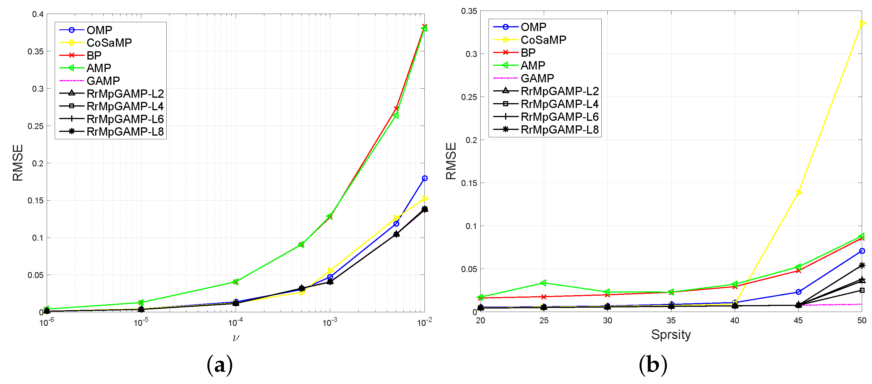
4.1. Zero-Mean Gaussian Projection Matrix Cases

In the first two experiments, the elements of $\mathbf{A}$ are independently drawn from $N(a;0,1/N)$, and the columns are normalized. The first experiment, termed the ν test, investigates the reconstruction performance versus noise power ν. Fixing $K=20$, the range of ν is $[{10}^{-6},{10}^{-5},{10}^{-4},5\times {10}^{-4},{10}^{-3},5\times {10}^{-3},{10}^{-2}]$. Figure 2a shows that four types $(L=2/4/6/8)$ of RrMpGAMP perform the same as GAMP, better than OMP and CoSaMP and much better than BP and AMP.

The second experiment, termed the sparsity test, investigates the reconstruction performance versus sparsity K. Fixing $SNR=40$ dB, the range of K is $[20,25,30,35,40,45,50]$. Figure 2b shows that four types $(L=2/4/6/8)$ of RrMpGAMP all perform the same as GAMP when $K\le 45$ or equally $\rho \le 0.35$. Notice that CoSaMP degrades obviously when $K\ge 40$, and RrMpGAMP-L4 is the best one in the $(M=128,N=256)$ setting, so we choose RrMpGAMP-L4 for the next three experiments.

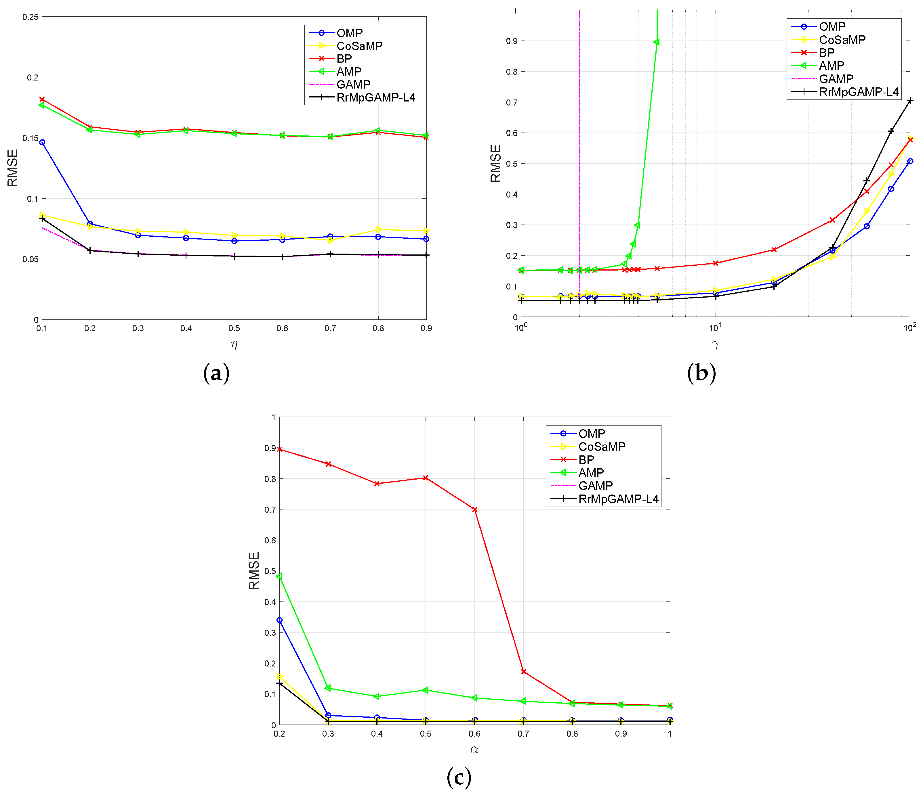
4.2. More General Projection Matrix Cases

The third experiment investigates the reconstruction performance of various sparse projection matrices. Define the sparsity ratio of matrix $\mathbf{A}$ as η; set the range of η to $[0.1,0.2,\cdots ,0.9]$; and fix $K=20$, $SNR=20$ dB. Figure 3a shows that RrMpGAMP-L4 performs the same as GAMP when $\eta >0.2$ and evidently better than the other four competitors.

For AMP and GAMP, although good performance can be achieved by zero-mean i.i.d. matrix $\mathbf{A}$, it tends to drastically decline even for a small positive bias. The fourth experiment, termed the γ test, shows this phenomenon. The elements of $\mathbf{A}$ are independently drawn from a Gaussian distribution $N(a;\gamma /N,1/N)$, where the mean is controlled by a positive parameter γ. Set the range of γ to $[1,1.6,1.8,2,2.2,2.4,3.4,3.6,3.8,4,5,10,20,40,60,80,100]$, and fix $K=20,SNR=20$ dB, Figure 3b shows that GAMP violently diverges at $\gamma =2$; AMP diverges at $\gamma =4$; but RrMpGAMP-L4 maintains good performance until $\gamma =40$. Although OMP, CoSaMP and BP also work well, RrMpGAMP-L4 performs a little better than OMP and CoSaMP when $\gamma <40$ and obviously better than BP.

The fifth experiment, termed the α test, considers an even more troublesome setup for strong correlated $\mathbf{A}$, and the elements of $\mathbf{A}$ are neither normal nor i.i.d. distributed. Fixing $K=12$, $SNR=30$ dB, the projection matrix is constructed by $\mathbf{A}=(1/N)\mathbf{P}\mathbf{Q}$. The elements of $\mathbf{P}$ and $\mathbf{Q}$ i.i.d. obey Gaussian distributions $p_{mr}\sim N(p;0,1)$ and $q_{rn}\sim N(q;0,1)$, where $\mathbf{P}\in {\mathbb{R}}^{M\times R},\mathbf{Q}\in {\mathbb{R}}^{R\times N}$ and $R\triangleq \lfloor \alpha N\rfloor$. The variation of α changes the size of $\mathbf{P}$ and $\mathbf{Q}$ and changes the rank of matrix $\mathbf{A}$. This means $\mathbf{A}$ is low rank for $\alpha <M/N$. Set the range of α to $[0.2,0.3,\cdots ,1.0]$. Since GAMP totally diverges ($\xi \approx {10}^6$) at every α, it is not visible in Figure 3c. This figure shows that RrMpGAMP-L4 keeps stable even in low rank scenario $\alpha \approx 0.3$, obviously better than AMP.

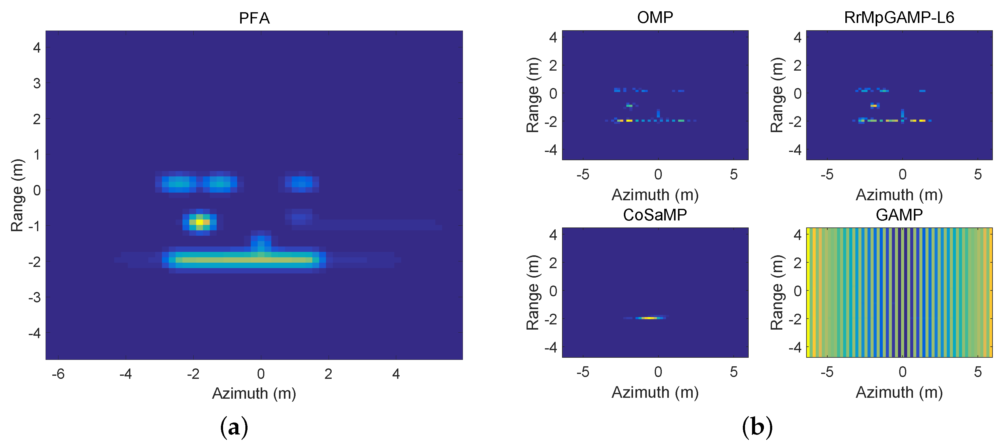
4.3. TomoSAR Imaging Application

The last experiment shows four TomoSAR imaging results. TomoSAR imaging is a spatial scatterer distribution reconstruction problem [28]. SAR imaging algorithms can be categorized into two classes: finding a dense solution and finding a sparse solution. The former is based on Nyquist sampling theory and discrete Fourier transform, e.g., the Polar Format Algorithm (PFA) [29,30]; the latter is based on compressed sampling theory and a sparse-induced algorithm, such as OMP. Tomography in the SAR imaging is especially used in inferring forest structure from several acquisitions taken at different view angles. The images are not sparse in that case. However, there are some reasons to motivate a compressed sensing TomoSAR radar, e.g., a target in a wild dry lake bed or the scatters of a target are very sparse. We simply describe the TomoSAR imaging model. The two-dimensional spatial spectrum of the TomoSAR echo is given by:

$$Y(f,\theta )={\int }_x{\int }_{y}g(x,y)exp\{-2jf(xcos\theta +ysin\theta )\}$$

(96)

where $f=2\pi /\lambda$ is the spatial frequency, $(x,y)$ is the position of a scatterer in the target coordinate, θ is the rotation angle between the radar coordinate and the target coordinate and $g(x,y)$ is the scattering coefficient. Using summation to replace integration, the discrete variables are: spatial frequency $\mathbf{f}\in {\mathbb{C}}^P$, where P is frequency sampling number; rotation angle $\mathbf{\theta }\in {\mathbb{C}}^Q$, where Q is the angle sampling number; scattering coefficient vector $\mathbf{x}\in {\mathbb{C}}^N$, which is composed of $g(x,y)$; where $N\ge P\times Q$ is the pixel number of a TomoSAR image; received echo signal $\mathbf{y}\in {\mathbb{C}}^M$; and complex Gaussian noise $\mathit{ϵ}\in {\mathbb{C}}^M$, where $M=P\times Q$. The linear system form of Equation (96) is the same as Equation (1). Define $F(p,q,n)\triangleq exp\{-2j{f}_p(x_{n}cos{\theta }_q+y_{n}sin{\theta }_q)\}$, and then:

$$\mathbf{A}=\left(\begin{array}{cccc}F(1,1,1)& F(1,1,2)& \cdots & F(1,1,N)\\ \cdots & \cdots & \cdots & \cdots \\ F(P,1,1)& F(P,1,2)& \cdots & F(P,1,N)\\ \cdots & \cdots & \cdots & \cdots \\ F(1,Q,1)& F(1,Q,2)& \cdots & F(1,Q,N)\\ \cdots & \cdots & \cdots & \cdots \\ F(P,Q,1)& F(P,Q,2)& \cdots & F(P,Q,N)\end{array}\right)$$

Because the scatterers are very sparse, it is feasible to randomly draw some rows from $\mathbf{A}$ to decrease P and Q, and to transform the TomoSAR imaging into a CS problem.

In this experiment, the TomoSAR echo data comes from a real-world crawler crane. $P=101$ frequency samples are spaced drawn from the $1(\text{GHz})$ bandwidth centered at carrier frequency $f_c=9(\text{GHz})$; $Q=101$ angle samples are spaced drawn from $87.5^{\circ }\sim 92.5^{\circ }$ centered at ${90}^{\circ }$ azimuth. The total pixels number is $N=P\times Q$. We draw $M=\lfloor 0.5N\rfloor$ rows from $\mathbf{A}$ randomly. Since the measurements number M is usually chosen to be $O(KlogN)$, K can be estimated roughly as $\tau M/logN$; we set $K=50$. Note that the elements of $\mathbf{A}$ and $\mathbf{y}$ are complex, so the prior of non-zero elements in $\mathbf{x}$ should be complex, as well.

Use the PFA imaging result in Figure 4a as the reference, and compare OMP, CoSaMP and GAMP to RrMpGAMP-L6. Figure 4b shows that CoSaMP and GAMP cannot recover the TomoSAR image; OMP and RrMpGAMP-L6 work well, but RrMpGAMP-L6 performs a little better than OMP; see the reconstructed bottom margin. RrMpGAMP-L6 recovers a more continuous segment than OMP.

5. Conclusions

While the AMP/GAMP algorithm has been shown to be a very good approach for sparse signal recovery, it is also sensitive to problems that deviate from its assumption. In this paper, we propose the stable RrMpGAMP algorithm, which matches GAMP’s accuracy, performs better than AMP and GAMP, and remains robust to various projection matrices, with a small memory footprint. We use the replica method to analyze the FsGAMP algorithm, which is embedded in the RrMpGAMP algorithm, and find that enlarging the variance range of the elements of the sensing matrix does not break the convergence property of FsGAMP. We also obtain the convergence conditions of FsGAMP. Experiments confirm that our proposed algorithm performs very well in simulation and practical problems for which AMP and GAMP cannot be applied. In all cases, RrMpGAMP provides better performance as compared to BP, OMP and CoSaMP. Exact analysis of the RrMP algorithm remains an open problem for future work.

References

1. Wu, Z.; Peng, S. Proportionate Minimum Error Entropy Algorithm for Sparse System Identification. Entropy 2015, 17, 5995–6006. [Google Scholar] [CrossRef]
2. Ma, W.; Qu, H. Maximum correntropy criterion based sparse adaptive filtering algorithms for robust channel estimation under non-Gaussian environments. J. Frankl. Inst. 2015, 352, 2708–2727. [Google Scholar] [CrossRef]
3. Ma, W.; Chen, B. Sparse least logarithmic absolute difference algorithm with correntropy induced metric penality. Circuit Syst. Signal Process. 2015, 35, 1077–1089. [Google Scholar] [CrossRef]
4. Chen, B.; Zhao, S. Online efficient learning with quantized KLMS and L1 regularization. In Proceedings of the International Joint Conference on Neural Networks, (IJCNN 2012), Brisbane, Australia, 10–15 June 2012; pp. 1–6.
5. Wang, W.X.; Yang, R.; Lai, Y.C.; Kovanis, V.; Grebogi, C. Predicting Catastrophes in Nonlinear Dynamical Systems by Compressive Sensing. Phys. Rev. Lett. 2011, 106. [Google Scholar] [CrossRef] [PubMed]
6. Brunton, S.L.; Tu, J.H.; Bright, I.; Kutz, J.N. Compressive Sensing and Low-Rank Libraries for Classification of Bifurcation Regimes in Nonlinear Dynamical Systems. SIAM J. Appl. Dyn. Syst. 2014, 13, 1716–1732. [Google Scholar] [CrossRef]
7. Donoho, D.; Maleki, A.; Motanari, A. Message Passing algorithms for compressed sensing. Proc. Natl. Acad. Sci. USA 2009, 106, 18914–18919. [Google Scholar] [CrossRef] [PubMed]
8. Donoho, D.; Maleki, A.; Montanari, A. Message passing algorithms for compressed sensing: I. motivation and construction. In Proceedings of the 2010 IEEE Information Theory Workshop (ITW), Cairo, Egypt, 6–8 January 2010; pp. 1–5.
9. Rangan, S. Generalized approximate message passing for estimation with random linear mixing. In Proceedings of the 2011 IEEE International Symposium on Information Theory Proceedings (ISIT), St. Petersburg, Russia, 31 July–5 August 2011; pp. 2168–2172.
10. Pati, Y.; Rezaiifar, R.; Krishnaprasad, P. Orthogonal matching pursuit: recursive function approximation with applications to wavelet decomposition. In Proceedings of the 1993 Conference Record of the Twenty-Seventh Asilomar Conference on Signals, Systems and Computers, Pacific Grove, CA, USA, 1–3 November 1993; Volume 1, pp. 40–44.
11. Needell, D.; Tropp, J.A. CoSaMP: Iterative signal recovery from incomplete and inaccurate samples. Appl. Comput. Harmonic Anal. 2009, 26, 301–321. [Google Scholar] [CrossRef]
12. Needell, D.; Vershynin, R. Uniform uncertainty principle and signal recovery via regularized orthogonal matching pursuit. Found. Comput. Math. 2009, 9, 317–334. [Google Scholar] [CrossRef]
13. Needell, D.; Vershynin, R. Signal recovery from incomplete and inaccurate measurements via regularized orthogonal matching pursuit. IEEE J. Sel. Top. Signal Process. 2010, 4, 310–316. [Google Scholar] [CrossRef]
14. Wainwright, M.J.; Jordan, M.I. Graphical models, exponential families, and variational inference. Found. Trends Mach. Learn. 2008, 1, 1–305. [Google Scholar] [CrossRef]
15. Rangan, S.; Schniter, P.; Fletcher, A. On the convergence of approximate message passing with arbitrary matrices. In Proceedings of the 2014 IEEE International Symposium on Information Theory (ISIT), Honolulu, HI, USA, 29 June–4 July 2014; pp. 236–240.
16. Golub, G.H.; van Loan, C.F. Matrix Computations, 3rd ed.; The Johns Hopkins University Press: Baltimore, MD, USA, 2012. [Google Scholar]
17. Ḿezard, M.; Parisi, G.; Virasoro, M.A. Spin-Glass Theory and Beyond. In World Scientific Lecture Notes in Physics; World Scientific: Singapore, Singapore, 1987; Volume 9. [Google Scholar]
18. Ḿezard, M.; Montanari, A. Information, Physics, and Computation; Oxford University Press: Oxford, UK, 2009. [Google Scholar]
19. Rangan, S.; Goyal, V.; Fletcher, A.K. Asymptotic analysis of map estimation via the replica method and compressed sensing. IEEE Trans. Inform. Theory 2012, 58, 1902–1923. [Google Scholar] [CrossRef] [Green Version]
20. Kabashima, Y.; Wadayama, T.; Tanaka, T. Statistical mechanical analysis of a typical reconstruction limit of compressed sensing. In Proceedings of the 2010 IEEE International Symposium on Information Theory (ISIT), Austin, TX, USA, 13–18 June 2010; pp. 1533–1537.
21. Ganguli, S.; Sompolinsky, H. Statistical mechanics of compressed sensing. Phys. Rev. Lett. 2010, 104. [Google Scholar] [CrossRef] [PubMed]
22. Solomon, A.T.; Bruhtesfa, E.G. Compressed Sensing Performance Analysis via Replica Method Using Bayesian framework. In Proceedings of the 17th UKSIM-AMSS International Conference on Modelling and Simulationm, Cambridge, UK, 25–27 March 2015; pp. 281–289.
23. Krzakala, F.; Mézard, M.; Sausset, F.; Sun, Y.; Zdeborová, L. Probabilistic reconstruction in compressed sensing: Algorithms, phase diagrams, and threshold achieving matrices. J. Stat. Mech. Theory Exp. 2012, 2012. [Google Scholar] [CrossRef]
24. Needell, D. Available online: http://www.cmc.edu/pages/faculty/DNeedell (accessed on 23 May 2016).
25. 1-MAGIC. Available online: http://users.ece.gatech.edu/ justin/l1magic (accessed on 23 May 2016).
26. Kamilov, U.S. Available online: http://www.ukamilov.com (accessed on 23 May 2016).
27. GAMP. Available online: http://gampmatlab.wikia.com/wiki/Generalized_Approximate_Message_Passing (accessed on 23 May 2016).
28. Zhu, X.X.; Bamler, R. Superresolving SAR Tomography for Multidimensional Imaging of Urban Areas: Compressive Sensing-Based TomoSAR inversion. IEEE Signal Process. Mag. 2014, 31, 51–58. [Google Scholar] [CrossRef]
29. Carrara, W.G.; Goodman, R.S.; Majewski, R.M. Spotlight Synthetic Aperture Radar: Signal Processing Algorithms; Artech House: Norwood, MA, USA, 1995. [Google Scholar]
30. Cong, X.; Liu, J.; Long, K.; Liu, Y.; Zhu, R.; Wan, Q. Millimeter-wave spotlight circular synthetic aperture radar (SCSAR) imaging for Foreign Object Debris on airport runway. In Proceedings of the 12th International Conference on Signal Processing (ICSP), HangZhou, China, 26–30 October 2014; pp. 1968–1972.
Figure 1. The factor graph description of a linear system. (a) Bipart factor graph; (b) Restricted factor graph.
Entropy 18 00207 g001
Figure 2. Reconstruction performance comparison using the zero-mean Gaussian projection matrix. (a) Noise power test; (b) Sparsity range test.
Entropy 18 00207 g002
Figure 3. Reconstruction performance comparison using three general form projection matrices. (a) Sparse matrix test; (b) Non-zero-mean matrix test; (c) Strong correlated matrix test.
Entropy 18 00207 g003
Figure 4. TomoSAR imaging results comparison using four Compressed Sensing (CS) algorithms and Polar Format Algorithm (PFA) algorithm as a reference. (a) PFA reconstructed image; (b) CS reconstructed images.
Entropy 18 00207 g004