Insights into Entropy as a Measure of Multivariate Variability

Abstract

Entropy has been widely employed as a measure of variability for problems, such as machine learning and signal processing. In this paper, we provide some new insights into the behaviors of entropy as a measure of multivariate variability. The relationships between multivariate entropy (joint or total marginal) and traditional measures of multivariate variability, such as total dispersion and generalized variance, are investigated. It is shown that for the jointly Gaussian case, the joint entropy (or entropy power) is equivalent to the generalized variance, while total marginal entropy is equivalent to the geometric mean of the marginal variances and total marginal entropy power is equivalent to the total dispersion. The smoothed multivariate entropy (joint or total marginal) and the kernel density estimation (KDE)-based entropy estimator (with finite samples) are also studied, which, under certain conditions, will be approximately equivalent to the total dispersion (or a total dispersion estimator), regardless of the data distribution.

1. Introduction

The concept of entropy can be used to quantify uncertainty, complexity, randomness, and regularity [1,2,3,4]. Particularly, entropy is also a measure of variability (or dispersion) of the associated distribution [5]. The most popular entropy functional is the Shannon entropy which is a central concept in information theory [1]. In addition to Shannon entropy, there are many other entropy definitions, such as Renyi and Tsallis entropies [2,3]. Renyi entropy is a generalized entropy which depends on a parameter $\alpha$ and includes Shannon entropy as a limiting case ($\alpha \to 1$). In this work, to simplify the discussion, we focus mainly on the Shannon and Renyi entropies.

Entropy has found applications in many fields such as statistics, physics, communication, ecology, etc. In the past decades, especially in recent years, entropy and related information theoretic measures (e.g., mutual information) have also been successfully applied in machine learning and signal processing [4,6,7,8,9,10]. Information theoretic quantities can capture higher-order statistics and offer potentially significant performance improvement in machine learning applications. In information theoretic learning (ITL) [4], the measures from information theory (entropy, mutual information, divergences, etc.) are often used as an optimization cost instead of the conventional second-order statistical measures such as variance and covariance. In particular, in many machine learning (supervised or unsupervised) problems, the goal is to optimize (maximize or minimize) the variability of the data, and in these cases one can optimize the entropy of the data so as to capture the underlying structure in the data. For example, in supervised learning, such as regression, the problem can be formulated as that of minimizing the entropy of the error between model output and desired response [11,12,13,14,15,16,17]. This optimization criterion is called in ITL the minimum error entropy (MEE) criterion [4,6].

In most practical applications, the data are multidimensional and multivariate. The total dispersion (i.e., the trace of the covariance matrix) and generalized variance (i.e., the determinant of the covariance matrix) are two widely used measures of multivariate variability, although both have some limitations [18,19,20]. However, these measures of multivariate variability involve only second-order statistics and cannot describe well non-Gaussian distributions. Entropy can be used as a descriptive and comprehensive measure of multivariate variability especially when data are non-Gaussian, since it can capture higher-order statistics and information content of the data rather than simply their energy [4]. There are strong relationships between entropy and traditional measures of multivariate variability (e.g., total dispersion and generalized variance). In the present work, we study this problem in detail and provide some new insights into the behavior of entropy as a measure of multivariate variability. We focus mainly on two types of multivariate entropy (or entropy power) measures, namely joint entropy and total marginal entropy. We show that for the jointly Gaussian case, the joint entropy and joint entropy power are equivalent to the generalized variance, while total marginal entropy is equivalent to the geometric mean of the marginal variances and total marginal entropy power is equivalent to the total dispersion. Further, we study the smoothed multivariate entropy measures and show that the smoothed joint entropy and smoothed total marginal entropy will be equivalent to a weighted version of total dispersion when the smoothing vector has independent entries and the smoothing factor approaches infinity. In particular, if the smoothing vector has independent and identically distributed entries, the two smoothed entropy measures will be equivalent to the total dispersion as the smoothing factor approaches infinity. Finally, we also show that with finite number of samples, the kernel density estimation (KDE) based entropy (joint or total marginal) estimator will be approximately equivalent to a total dispersion estimator if the kernel function is Gaussian with covariance matrix being an identity matrix and the smoothing factor is large enough.

The rest of the paper is organized as follows. In Section 2, we present some entropy measures of multivariate variability and discuss the relationships between entropy and traditional measures of multivariate variability. In Section 3, we study the smoothed multivariate entropy measures and gain insights into the links between the smoothed entropy and total dispersion. In Section 4, we investigate the KDE based entropy estimator (with finite samples), and prove that under certain conditions the entropy estimator is approximately equivalent to a total dispersion estimator. Finally in Section 5, we give the conclusion.

2. Entropy Measuresfor Multivariate Variability

2.1. Shannon’s Entropy

Entropy has long been employed as a measure of variability (spread, dispersion, or scatter) of a distribution [5]. A common measure of multivariate variability is the joint entropy (JE). Given a d-dimensional random vector $X=\left[X_1,\cdots ,X_d\right]\in {ℝ}^d$, with probability density function (PDF) $p_X(x)$, where $x=\left[x_1,\cdots ,x_d\right]$, Shannon’s joint entropy of $X$ is defined by [1]:

$$H(X)=-{\displaystyle {\int }_{{ℝ}^d}{p}_X(x)\log p_X(x)dx}$$

(1)

Another natural measure of multivariate variability is the Total Marginal Entropy (TME), defined as:

$$T(X)={\displaystyle \sum _{i=1}^{d}H(X_i)}=-{\displaystyle \sum _{i=1}^d{\displaystyle {\int }_{ℝ}{p}_{X_i}(x_i)\log p_{X_i}(x_i)d{x}_i}}$$

(2)

where $p_{X_i}(x_i)$ denotes the marginal density, and $H(X_i)$ the corresponding marginal entropy. We have $T(X)\ge H(X)$, with equality if and only if all elements of $X$ are independent. Further, the following theorem holds.

Theorem 1. 

If $X$ is jointly Gaussian, with PDF:

$$p_X(x)=\frac{1}{{(2\pi )}^{d/2}{|\Sigma |}^{1/2}}\exp \left(-\frac{1}{2}{\left(x-\mu \right)}^T{\Sigma }^{-1}\left(x-\mu \right)\right)$$

(3)

where $\mu$ denotes the mean vector, $\Sigma$ stands for the covariance matrix, and $|\Sigma |$ denotes the determinant of $\Sigma$, then:

$$H(X)=\frac{d}{2}\log 2\pi +\frac{d}{2}+\frac{1}{2}\log |\Sigma |$$

(4)

$$T(X)=\frac{d}{2}\log 2\pi +\frac{d}{2}+\frac{1}{2}\log {\displaystyle \prod _{i=1}^d{\Sigma }_{ii}}$$

(5)

where ${\Sigma }_{ii}$ denotes the i-th diagonal element of $\Sigma$, i.e., the variance of $X_i$.

Proof. 

Using Equation (3), we derive:

$$\begin{array}{cc}\hfill H(X)& =-{\displaystyle {\int }_{{ℝ}^d}{p}_X(x)\log p_X(x)dx}\hfill \\ & =-{\displaystyle {\int }_{{ℝ}^d}{p}_X(x)\log \left(\frac{1}{{(2\pi )}^{d/2}{|\Sigma |}^{1/2}}\exp \left(-\frac{1}{2}{\left(x-\mu \right)}^T{\Sigma }^{-1}\left(x-\mu \right)\right)\right)dx}\hfill \\ & =\log \left({(2\pi )}^{d/2}{|\Sigma |}^{1/2}\right){\displaystyle {\int }_{{ℝ}^d}{p}_X(x)dx}+\frac{1}{2}{\displaystyle {\int }_{{ℝ}^d}{\left(x-\mu \right)}^T{\Sigma }^{-1}\left(x-\mu \right)p_X(x)dx}\hfill \\ & =\frac{d}{2}\log 2\pi +\frac{1}{2}\log |\Sigma |+\frac{1}{2}Tr\left({\Sigma }^{-1}\Sigma \right)\hfill \\ & =\frac{d}{2}\log 2\pi +\frac{d}{2}+\frac{1}{2}\log |\Sigma |\hfill \end{array}$$

where $Tr(.)$ denotes the trace operator. In a similar way, we get:

$$\begin{array}{cc}\hfill T(X)& ={\displaystyle \sum _{i=1}^{d}H(X_i)}\hfill \\ & ={\displaystyle \sum _{i=1}^d\left(\frac{1}{2}\log 2\pi +\frac{1}{2}+\frac{1}{2}\log {\Sigma }_{ii}\right)}\hfill \\ & =\frac{d}{2}\log 2\pi +\frac{d}{2}+\frac{1}{2}\log {\displaystyle \prod _{i=1}^d{\Sigma }_{ii}}\hfill \end{array}$$

□

Remark 1. 

Since the logarithm is a monotonic function, for the jointly Gaussian case, the joint entropy $H(X)$ is equivalent to the generalized variance (GV), namely the determinant of $\Sigma$ [18,19,20], and the total marginal entropy $T(X)$ is equivalent to the geometric mean of the $d$ marginal variances (${\left({\displaystyle \prod _{i=1}^d{\Sigma }_{ii}}\right)}^{1/d}$). The concept of the generalized variance, which can be traced back to Wilks [21], was suggested by Sokal [22] to measure the overall variability in multivariate biometrical studies, and was applied by Goodman [23] to get easily interpretable results on corn and cotton populations, and recently was also applied by Barrett, Barnett, and Seth [24,25] to multivariate Granger Causality analysis. The generalized variance plays an important role in Maximum Likelihood Estimation (MLE) and model selection. Some limitations of the generalized variance, however, were discussed in [18,19,20].

The covariance matrix $\Sigma$ can be expressed as:

$$\Sigma =\Delta \mathrm{P}\Delta$$

(6)

where $\mathrm{P}$ is the correlation matrix, and $\Delta$ is a diagonal matrix with the $d$ marginal standard deviations, $\sqrt{{\Sigma }_{ii}}$, along the diagonal. Thus, the generalized variance and the geometric mean of the marginal variances have the following relationship:

$$|\Sigma |=\left|\mathrm{P}\right|{\displaystyle \prod _{i=1}^d{\Sigma }_{ii}}$$

(7)

where $\left|\mathrm{P}\right|$ is the determinant of $\mathrm{P}$. From Equation (7), one can see that the generalized variance depends on both $\left|\mathrm{P}\right|$ and the geometric mean of the marginal variances. If the correlation matrix $\mathrm{P}$ is near-singular, however, the generalized variance will collapse to a very small value regardless of the values of the marginal variances. This is a significant disadvantage of the generalized variance [18].

Remark 2. 

Although for the jointly Gaussian case, there is a simple relationship between the entropy based measures of variability and the traditional variance based measures, the two kinds of measures are quite different. The entropy may be related to higher-order moments of a distribution and can provide a much more comprehensive characterization of the distribution. Only when the distribution (e.g., Gaussian) can be well characterized by the first two moments, or when a quadratic approximation is satisfactory, the variance based measures are justifiable [4,6].

2.2. Renyi's Entropy

There are many extensions to Shannon’s measure of entropy. Renyi’s entropy of order-$\alpha$ is a well-known generalization of Shannon entropy [2,4]. Based on Renyi’s definition of entropy, the order-$\alpha$ joint entropy and total marginal entropy of $X$ are:

$$H_{\alpha }(X)=\frac{1}{1-\alpha }\log V_{\alpha }(X)$$

(8)

$$T_{\alpha }(X)={\displaystyle \sum _{i=1}^d{H}_{\alpha }(X_i)}=\frac{1}{1-\alpha }\log {\displaystyle \prod _{i=1}^d{V}_{\alpha }(X_i)}$$

(9)

where $\alpha >0$, $\alpha \ne 1$, and $V_{\alpha }(X)$ denotes the order-$\alpha$ Information Potential (IP) [4] of $X$:

$$V_{\alpha }(X)={\displaystyle {\int }_{{ℝ}^d}{p}_X^{\alpha }(x)dx}$$

(10)

Remark 3. 

In recent years, Renyi’s entropy of order-$\alpha$ is widely accepted as an optimality criterion in Information Theoretic Learning (ITL) [4]. The nonparametric kernel (Parzen window) estimator of Renyi entropy (especially when $\alpha =2$) has been shown to be more computationally efficient than that of Shannon entropy [11,12].

Remark 4. 

The information potential is actually the Information Generating Function defined in [26]. It is called information potential since each term in its kernel estimator can be interpreted as a potential between two particles [4]. As the logarithm is a monotonic function, minimizing Renyi entropy is equivalent to minimizing (when $\alpha <1$) or maximizing (when $\alpha >1$) the information potential. Thus, the information potential can be used as an alternative to Renyi entropy as a measure of variability.

It is easy to verify that Renyi’s entropy will approach Shannon’s entropy as $\alpha \to 1$. In addition, Theorem 1 can be extended to the Renyi entropy case.

Theorem 2. 

If $X$ is jointly Gaussian, with PDF given by Equation (3), then:

$$H_{\alpha }(X)=\frac{d}{1-\alpha }\log \beta +\frac{1}{2}\log |\Sigma |$$

(11)

$$T_{\alpha }(X)=\frac{d}{1-\alpha }\log \beta +\frac{1}{2}\log {\displaystyle \prod _{i=1}^d{\Sigma }_{ii}}$$

(12)

where $\beta ={(2\pi )}^{\frac{(1-\alpha )}{2}}{\alpha }^{-\frac{1}{2}}$.

Proof. 

One can derive:

$$\begin{array}{cc}\hfill V_{\alpha }(X)& ={\displaystyle {\int }_{{ℝ}^d}{p}_X^{\alpha }(x)dx}\hfill \\ & ={\displaystyle {\int }_{{ℝ}^d}{\left(\frac{1}{{(2\pi )}^{d/2}{|\Sigma |}^{1/2}}\exp \left(-\frac{1}{2}{\left(x-\mu \right)}^T{\Sigma }^{-1}\left(x-\mu \right)\right)\right)}^{\alpha }dx}\hfill \\ & =\frac{1}{{(2\pi )}^{\alpha d/2}{|\Sigma |}^{\alpha /2}}{\displaystyle {\int }_{{ℝ}^d}\exp \left(-\frac{1}{2}{\left(x-\mu \right)}^T{\left({\alpha }^{-1}\Sigma \right)}^{-1}\left(x-\mu \right)\right)dx}\hfill \\ & =\frac{1}{{(2\pi )}^{\alpha d/2}{|\Sigma |}^{\alpha /2}}\times {(2\pi )}^{d/2}{\left|{\alpha }^{-1}\Sigma \right|}^{1/2}\hfill \\ & ={\beta }^d{|\Sigma |}^{(1-\alpha )/2}\hfill \end{array}$$

(13)

Similarly, we have:

$$V_{\alpha }(X_i)=\beta {{\Sigma }_{ii}}^{(1-\alpha )/2}$$

(14)

Substituting Equations (13) and (14) into Equations (8) and (9), respectively, yields Equations (11) and (12). □

Remark 5. 

From Theorem 2 we find that, for the jointly Gaussian case, Renyi’s joint entropy $H_{\alpha }(X)$ is also equivalent to the generalized variance $|\Sigma |$, and the order-$\alpha$ total marginal entropy $T_{\alpha }(X)$ is equivalent to the geometric mean of the $d$ marginal variances.

2.3. Entropy Powers

In [5], the variability (or the extent) of a distribution was measured by the exponential entropy, or equivalently, the entropy power. Shannon and Renyi’s joint entropy powers (JEP) are defined by [27]:

$$N(X)=\exp \left[\frac{2}{d}H(X)\right]$$

(15)

$$N_{\alpha }(X)=\exp \left[\frac{2}{d}{H}_{\alpha }(X)\right]$$

(16)

Similarly, the total marginal entropy powers (TMEP) are:

$$M(X)={\displaystyle \sum _{i=1}^{d}N(X_i)}={\displaystyle \sum _{i=1}^d\exp \left[2H(X_i)\right]}$$

(17)

$$M_{\alpha }(X)={\displaystyle \sum _{i=1}^d{N}_{\alpha }(X_i)}={\displaystyle \sum _{i=1}^d\exp \left[2H_{\alpha }(X_i)\right]}$$

(18)

Clearly, we have $N(X)=\underset{\alpha \to 1}{\lim }{N}_{\alpha }(X)$, $M(X)=\underset{\alpha \to 1}{\lim }{M}_{\alpha }(X)$. The following theorem holds.

Theorem 3. 

If $X$ is jointly Gaussian, with PDF given by Equation (3), then:

$$N(X)=2\pi e{|\Sigma |}^{\frac{1}{d}}$$

(19)

$$N_{\alpha }(X)={\beta }^{\frac{2}{1-\alpha }}{|\Sigma |}^{\frac{1}{d}}$$

(20)

$$M(X)=2\pi eTr(\Sigma )$$

(21)

$$M_{\alpha }(X)={\beta }^{\frac{2}{1-\alpha }}Tr(\Sigma )$$

(22)

Proof. 

Since $H(X)=\frac{d}{2}\log 2\pi +\frac{d}{2}+\frac{1}{2}\log |\Sigma |$, $H_{\alpha }(X)=\frac{d}{1-\alpha }\log \beta +\frac{1}{2}\log |\Sigma |$, $H(X_i)=\frac{1}{2}\log 2\pi +\frac{1}{2}+\frac{1}{2}\log {\Sigma }_{ii}$, and $H_{\alpha }(X_i)=\frac{1}{1-\alpha }\log \beta +\frac{1}{2}\log {\Sigma }_{ii}$, we have:

$$N(X)=\exp \left[\frac{2}{d}H(X)\right]=2\pi e{|\Sigma |}^{\frac{1}{d}}$$

$$N_{\alpha }(X)=\exp \left[\frac{2}{d}{H}_{\alpha }(X)\right]={\beta }^{\frac{2}{1-\alpha }}{|\Sigma |}^{\frac{1}{d}}$$

$$M(X)={\displaystyle \sum _{i=1}^d\exp \left[2H(X_i)\right]}=2\pi eTr(\Sigma )$$

$$M_{\alpha }(X)={\displaystyle \sum _{i=1}^d\exp \left[2H_{\alpha }(X_i)\right]}={\beta }^{\frac{2}{1-\alpha }}Tr(\Sigma )$$

□

Remark 6. 

For the jointly Gaussian case, the joint entropy powers $N(X)$ and $N_{\alpha }(X)$ are equivalent to the generalized variance $|\Sigma |$, and the total marginal entropy powers $M(X)$ and $M_{\alpha }(X)$ are equivalent to the well-known total dispersion (TD) or total variation (TV), given by $Tr(\Sigma )={\displaystyle \sum _{i=1}^d{\Sigma }_{ii}}$ [19]. The total dispersion is widely accepted as a measure of variation in regression, clustering, and principal components analysis (PCA). Let ${\lambda }_1$, ${\lambda }_2$, ..., ${\lambda }_d$ be the eigenvalues of the covariance matrix $\Sigma$. Then the generalized variance and total dispersion can be expressed as:

$$|\Sigma |={\displaystyle \prod _{i=1}^d{\lambda }_i}, Tr(\Sigma )={\displaystyle \sum _{i=1}^d{\lambda }_i}$$

(23)

Table 1 lists Renyi’s entropy (which includes Shannon’s entropy as a special case) based measures of variability and their equivalent variance based measures (for the jointly Gaussian case).

Table 1. Renyi’s entropy based measures of variability and their equivalent variance based measures.

Entropy Based Measures	Equivalent Variance Based Measures
Renyi’s Joint Entropy: $H_{\alpha }(X)$	Generalized Variance: $|\Sigma |$
Renyi’s Total Marginal Entropy: $T_{\alpha }(X)$	Geometric Mean of Marginal Variances: ${\left({\displaystyle \prod _{i=1}^d{\Sigma }_{ii}}\right)}^{1/d}$
Renyi’s Joint Entropy Power: $N_{\alpha }(X)$	Generalized Variance: $|\Sigma |$
Renyi’s Total Marginal Entropy Power: $M_{\alpha }(X)$	Total Dispersion: $Tr(\Sigma )$

3. Smoothed Multivariate Entropy Measures

In most practical situations, the analytical evaluation of the entropy is not possible, and one has to estimate its value from the samples. So far there are many entropy estimators, among which the k-nearest neighbors based estimators are important ones in a wide range of practical applications [28]. In ITL, however, the kernel density estimation (KDE) based estimators are perhaps the most popular ones due to their smoothness [4]. By KDE approach [29], with a fixed kernel function, the estimated entropy will converge asymptotically to the entropy of the underlying random variable plus an independent random variable whose PDF corresponds to the kernel function [4]. This asymptotic value of entropy is called the smoothed entropy [16]. In this section, we will investigate some interesting properties of the smoothed multivariate entropy (joint or total marginal) as a measure of variability. Unless mentioned otherwise, the smoothed entropy studied in the following is based on the Shannon entropy, but the obtained results can be extended to many other entropies.

Given a $d$-dimensional random vector $X=\left[X_1,\cdots ,X_d\right]\in {ℝ}^d$, with PDF $p_X(x)$, and a smoothing vector $Z=\left[Z_1,\cdots ,Z_d\right]\in {ℝ}^d$ that is independent of $X$ and has PDF $p_Z(x)$, the smoothed joint entropy of $X$, with smoothing factor $\lambda$ ($\lambda >0$), is defined by [16]:

$$H_{\lambda Z}\left(X\right)=H\left(X+\lambda Z\right)=-{\displaystyle {\int }_{{ℝ}^d}{p}_{X+\lambda Z}(x)\log p_{X+\lambda Z}(x)dx}$$

(24)

where $p_{X+\lambda Z}(x)$ denotes the PDF of $X+\lambda Z$, which is:

$$p_{X+\lambda Z}(x)=p_X(x)\circ p_{\lambda Z}(x)$$

(25)

where “$\circ$” denotes the convolution operator, and $p_{\lambda Z}(x)=\frac{1}{{\lambda }^d}{p}_Z(\frac{x}{\lambda })$ is the PDF of $\lambda Z$.

Let $\left\{x(1),x(2),\cdots ,x(N)\right\}$ be $N$ independent, identically distributed (i.i.d.) samples drawn from $p_X(x)$. By KDE approach, with a fixed kernel function $p_Z(.)$, the estimated PDF of $X$ will be [29]:

$${\widehat{p}}_X(x)=\frac{1}{N{\lambda }^d}{\displaystyle \sum _{k=1}^N{p}_Z\left(\frac{x-x(k)}{\lambda }\right)}$$

(26)

where $\lambda >0$ is the smoothing factor (or kernel width). As sample number $N\to \infty$, the estimated PDF will uniformly converge (with probability 1) to the true PDF convolved with the kernel function. So we have:

$${\widehat{p}}_X(x)\stackrel{N\to \infty }{\to }{p}_{X+\lambda Z}(x)$$

(27)

Plugging the above estimated PDF into the entropy definition, one may obtain an estimated entropy of $X$, which converges, almost surely (a.s.), to the smoothed entropy $H_{\lambda Z}\left(X\right)$.

Remark 7. 

Theoretically, using a suitable annealing rate for the smoothing factor $\lambda$, the KDE based entropy estimator can be asymptotically unbiased and consistent [29]. In many machine learning applications, however, the smoothing factor is often kept fixed. The main reasons for this are basically two: (1) in practical situations, the training data are always finite; (2) in general the learning seeks extrema (either minimum or maximum) of the cost function, independently to its actual value, and the dependence on the estimation bias is decreased. Therefore, the study of the smoothing entropy will help us to gain insights into the asymptotic behaviors of the entropy based learning.

Similarly, one can define the Smoothed Total Marginal Entropy of $X$:

$$T_{\lambda Z}(X)={\displaystyle \sum _{i=1}^d{H}_{\lambda Z_i}(X_i)}=-{\displaystyle \sum _{i=1}^d{\displaystyle {\int }_{ℝ}{p}_{X_i+\lambda Z_i}(x)\log p_{X_i+\lambda Z_i}(x)dx}}$$

(28)

where $p_{X_i+\lambda Z_i}(x)$ denotes the smoothed marginal density, $p_{X_i+\lambda Z_i}(x)=p_{X_i}(x)\circ p_{\lambda Z_i}(x)$.

The smoothing factor $\lambda$ is a very important parameter in the smoothed entropy measures (joint or total marginal). As $\lambda \to 0$, the smoothed entropy measures will reduce to the original entropy measures, $\underset{\lambda \to 0}{\lim }{H}_{\lambda Z}\left(X\right)=H\left(X\right)$, $\underset{\lambda \to 0}{\lim }{T}_{\lambda Z}\left(X\right)=T\left(X\right)$. In the following, we study the case in which $\lambda$ is very large. Before presenting Theorem 4, we introduce an important lemma.

Lemma 1. 

(De Bruijn's Identity [30]): For any two independent random d-dimensional vectors, $X$ and $Z$, with PDFs $p_X$ and $p_Z$, such that $J(X)$ exists and $Z$ has finite covariance, where $J(X)$ denotes the $d\times d$ Fisher Information Matrix (FIM):

$$J(X)=E\left[S(X)S{(X)}^T\right]$$

(29)

in which $S(X)=\frac{1}{p_X(X)}\frac{\partial }{\partial X}{p}_X(X)$ is the zero-mean Score of $X$, then:

$${\frac{d}{dt}H(X+\sqrt{t}Z)|}_{t=0}=\frac{1}{2}Tr\left(J(X){\Sigma }_Z\right)$$

(30)

where ${\Sigma }_Z$ denotes the $d\times d$ covariance matrix of $Z$.

Theorem 4. 

As $\lambda$ is large enough, we have:

$$H_{\lambda Z}(X)\approx H(Z)+\frac{1}{2}Tr\left(J(Z){\Sigma }_X\right)t-\frac{d}{2}\log t$$

(31)

$$T_{\lambda Z}(X)\approx {\displaystyle \sum _{i=1}^{d}H(Z_i)}+\frac{t}{2}{\displaystyle \sum _{i=1}^{d}J(Z_i){\sigma }_{X_i}^2}-\frac{d}{2}\log t$$

(32)

where $t=1/{\lambda }^2$, and ${\sigma }_{X_i}^2$ denotes the variance of $X_i$.

Proof. 

The smoothed joint entropy $H_{\lambda Z}(X)$ can be rewritten as:

$$H_{\lambda Z}\left(X\right)=H\left(X+\lambda Z\right)=H\left(\lambda \left(\frac{1}{\lambda }X+Z\right)\right)=H\left(\frac{1}{\lambda }X+Z\right)+d\log \lambda$$

(33)

Let $t=1/{\lambda }^2$, we have:

$$H_{\lambda Z}\left(X\right)=H\left(\sqrt{t}X+Z\right)-\frac{d}{2}\log t$$

(34)

Then, by De Bruijn’s Identity:

$$\begin{array}{cc}\hfill H_{\lambda Z}\left(X\right)& =H(Z)+{\frac{d}{dt}H\left(\sqrt{t}X+Z\right)|}_{t=0}t-\frac{d}{2}\log t+o(t)\hfill \\ & =H(Z)+\frac{1}{2}Tr\left(J(Z){\Sigma }_X\right)t-\frac{d}{2}\log t+o(t)\hfill \end{array}$$

(35)

where $o(t)$ denotes the higher-order infinitesimal term of the Taylor expansion. Similarly, one can easily derive:

$$T_{\lambda Z}(X)={\displaystyle \sum _{i=1}^{d}H(Z_i)}+\frac{t}{2}{\displaystyle \sum _{i=1}^{d}J(Z_i){\sigma }_{X_i}^2}-\frac{d}{2}\log t+o(t)$$

(36)

Thus, as $\lambda$ is large enough, $t$ will be very small, such that Equations (31) and (32) hold. □

Remark 8. 

In Equation (31), the term $\left\{H(Z)-\frac{d}{2}\log t\right\}$ is not related to $X$. So, when the smoothing factor $\lambda$ is large enough, the smoothed joint entropy $H_{\lambda Z}\left(X\right)$ will be, approximately, equivalent to $Tr\left(J(Z){\Sigma }_X\right)$, denoted by:

$$H_{\lambda Z}\left(X\right)\stackrel{\lambda \to \infty }{\rightleftharpoons }Tr\left(J(Z){\Sigma }_X\right)$$

(37)

Similarly, we have:

$$T_{\lambda Z}(X)\stackrel{\lambda \to \infty }{\rightleftharpoons }{\displaystyle \sum _{i=1}^{d}J(Z_i){\sigma }_{X_i}^2}$$

(38)

In the following, we consider three special cases of the smoothing vector $Z$.

Case 1. 

If $Z$ is a jointly Gaussian random vector, then $J(Z)={\Sigma }_Z^{-1}$, and $J(Z_i)=1/{\sigma }_{Z_i}^2$, where ${\sigma }_{Z_i}^2$ denotes the variance of $Z_i$. In this case, we have:

$$H_{\lambda Z}\left(X\right)\stackrel{\lambda \to \infty }{\rightleftharpoons }Tr\left({\Sigma }_Z^{-1}{\Sigma }_X\right)$$

(39)

$$T_{\lambda Z}(X)\stackrel{\lambda \to \infty }{\rightleftharpoons }{\displaystyle \sum _{i=1}^d{\sigma }_{X_i}^2/{\sigma }_{Z_i}^2}$$

(40)

Case 2. 

If $Z$ has independent entries, then $J(Z)$ is a diagonal matrix, with $J(Z_i)$ along the diagonal. It follows easily that:

$$H_{\lambda Z}\left(X\right)\stackrel{\lambda \to \infty }{\rightleftharpoons }{T}_{\lambda Z}(X)\stackrel{\lambda \to \infty }{\rightleftharpoons }{\displaystyle \sum _{i=1}^{d}J(Z_i){\sigma }_{X_i}^2}$$

(41)

Case 3. 

If $Z$ has independent and identically distributed (i.i.d.) entries, then $J(Z)=J(Z_1)I$, where $I$ is a $d\times d$ identity matrix. Thus:

$$H_{\lambda Z}\left(X\right)\stackrel{\lambda \to \infty }{\rightleftharpoons }{T}_{\lambda Z}(X)\stackrel{\lambda \to \infty }{\rightleftharpoons }{\displaystyle \sum _{i=1}^d{\sigma }_{X_i}^2}$$

(42)

Remark 9. 

It is interesting to observe that, if the smoothing vector $Z$ has independent entries, then the smoothed joint entropy and smoothed total marginal entropy will be equivalent to each other as $\lambda \to \infty$. In this case, they are both equivalent to a weighted version of total dispersion, with weights $J(Z_i)$. In particular, when $Z$ has i.i.d. entries, the two entropy measures will be equivalent (as $\lambda \to \infty$) to the ordinary total dispersion. Note that the above results hold even if $X$ is non-Gaussian distributed. The equivalent measures of the smoothed joint and total marginal entropies as $\lambda \to \infty$ are summarized in Table 2.

Table 2. Equivalent measures of the smoothed joint and total marginal entropies as $\lambda \to \infty$.

	Smoothed Joint Entropy	Smoothed Total Marginal Entropy
General case	$Tr\left(J(Z){\Sigma }_X\right)$	${\displaystyle \sum _{i=1}^{d}J(Z_i){\sigma }_{X_i}^2}$
If $Z$ is jointly Gaussian	$Tr\left({\Sigma }_Z^{-1}{\Sigma }_X\right)$	${\displaystyle \sum _{i=1}^d{\sigma }_{X_i}^2/{\sigma }_{Z_i}^2}$
If $Z$ has independent entries	${\displaystyle \sum _{i=1}^{d}J(Z_i){\sigma }_{X_i}^2}$	${\displaystyle \sum _{i=1}^{d}J(Z_i){\sigma }_{X_i}^2}$
If $Z$ has i.i.d. entries	${\displaystyle \sum _{i=1}^d{\sigma }_{X_i}^2}$	${\displaystyle \sum _{i=1}^d{\sigma }_{X_i}^2}$

Example 1. 

According to Theorem 4, if $Z$ has independent entries, the smoothed joint entropy $H_{\lambda Z}\left(X\right)$ and the smoothed total marginal entropy $T_{\lambda Z}(X)$ will approach a same value with $\lambda$ increasing. Below we present a simple example to confirm this fact.

Consider a two-dimensional case in which $X$ is mixed-Gaussian with PDF:

$$p_X(x)=\frac{1}{4\pi \sqrt{1-{\rho }^2}}\left\{\exp \left(-\frac{x_2^2-2\rho x_2(x_1-\mu )+{(x_1-\mu )}^2}{2(1-{\rho }^2)}\right)+\exp \left(-\frac{x_2^2+2\rho x_2(x_1+\mu )+{(x_1+\mu )}^2}{2(1-{\rho }^2)}\right)\right\}$$

where $\mu =0.5$, $\rho =0.95$, and $Z$ is uniformly distributed over $[-1.0,1.0]\times [-1.0,1.0]$. Figure 1 illustrates the smoothed entropies (joint and total marginal) with different $\lambda$ values. As one can see clearly, when $\lambda$ is small (close to zero), the smoothed total marginal entropy is larger than the smoothed joint entropy, and the difference is significant; while when $\lambda$ gets larger (say, larger than 2.0), the discrepancy between the two entropy measures will disappear.

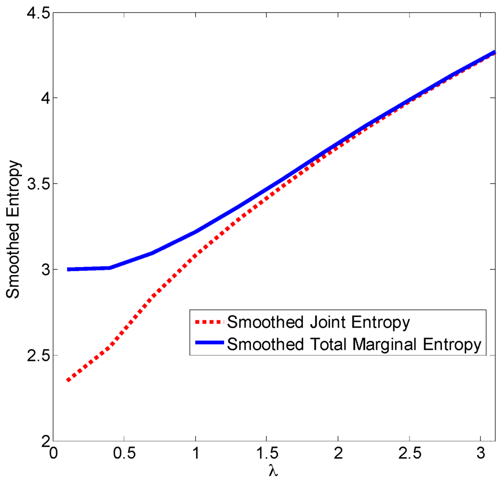
Figure 1. Smoothed entropies with different smoothing factors.

4. Multivariate Entropy Estimators with Finite Samples

The smoothed entropy is of only theoretical interest since in practical applications, the number of samples is always limited, and the asymptotic value of the entropy estimator can never be reached. In the following, we show, however, that similar results hold for finite samples case. Consider again the kernel density estimator Equation (26). For simplicity we assume that the kernel function is Gaussian with covariance matrix ${\Sigma }_Z=I$, where $I$ is a $d\times d$ identity matrix. In this case, the estimated PDF of $X$ becomes:

$$\begin{array}{cc}\hfill {\widehat{p}}_X(x)& =\frac{1}{N}{\left(\frac{1}{\sqrt{2\pi }\lambda }\right)}^d{\displaystyle \sum _{k=1}^N\exp \left(-\frac{{\Vert x-x(k)\Vert }^2}{2{\lambda }^2}\right)}\hfill \\ & =\frac{1}{N}{\left(\frac{1}{\sqrt{2\pi }\lambda }\right)}^d{\displaystyle \sum _{k=1}^N{\displaystyle \prod _{i=1}^d\exp \left(-\frac{{\left(x_i-x_i(k)\right)}^2}{2{\lambda }^2}\right)}}\hfill \end{array}$$

(43)

where $x_i$ denotes the i-th element of vector $x$. With the above estimated PDF, a sample-mean estimator of the joint entropy $H(X)$ is [4]:

$$\begin{array}{cc}\hfill \widehat{H}(X)& =-\frac{1}{N}{\displaystyle \sum _{j=1}^N\log {\widehat{p}}_X(x(j))}\hfill \\ & =-\frac{1}{N}{\displaystyle \sum _{j=1}^N\log \left\{\frac{1}{N}{\left(\frac{1}{\sqrt{2\pi }\lambda }\right)}^d{\displaystyle \sum _{k=1}^N\exp \left(-\frac{{\Vert x(j)-x(k)\Vert }^2}{2{\lambda }^2}\right)}\right\}}\hfill \end{array}$$

(44)

Similarly, an estimator for the total marginal entropy can be obtained as follows:

$$\widehat{T}(X)={\displaystyle \sum _{i=1}^d\left(-\frac{1}{N}{\displaystyle \sum _{j=1}^N\log \left\{\frac{1}{N}{\displaystyle \sum _{k=1}^N\frac{1}{\sqrt{2\pi }\lambda }\exp \left(-\frac{{\left(x_i(j)-x_i(k)\right)}^2}{2{\lambda }^2}\right)}\right\}}\right)}$$

(45)

The following theorem holds.

Theorem 5. 

As $\lambda$ is large enough, we have:

$$\widehat{H}(X)\approx \widehat{T}(X)\approx d\log \left(\sqrt{2\pi }\lambda \right)+\frac{1}{{\lambda }^2}{\displaystyle \sum _{i=1}^d{\widehat{\sigma }}_{X_i}^2}$$

(46)

where ${\widehat{\sigma }}_{X_i}^2=\frac{1}{N}{{\displaystyle \sum _{j=1}^N\left[x_i(j)-\frac{1}{N}{\displaystyle \sum _{k=1}^N{x}_i(k)}\right]}}^2$ is the estimated variance of $X_i$.

Proof. 

When $\lambda \to \infty$, we have $\frac{{\Vert x(j)-x(k)\Vert }^2}{2{\lambda }^2}\to 0$. It follows that:

$$\begin{array}{cc}\widehat{H}(X)& =d\log \left(\sqrt{2\pi }\lambda \right)-\frac{1}{N}{\displaystyle \sum _{j=1}^N\log \left\{\frac{1}{N}{\displaystyle \sum _{k=1}^N\exp \left(-\frac{{\Vert x(j)-x(k)\Vert }^2}{2{\lambda }^2}\right)}\right\}}\hfill \\ & \stackrel{(a)}{\approx }d\log \left(\sqrt{2\pi }\lambda \right)-\frac{1}{N}{\displaystyle \sum _{j=1}^N\log \left(1-\frac{1}{N}{\displaystyle \sum _{k=1}^N\frac{{\Vert x(j)-x(k)\Vert }^2}{2{\lambda }^2}}\right)}\hfill \\ & \stackrel{(b)}{\approx }d\log \left(\sqrt{2\pi }\lambda \right)+\frac{1}{N^2}{\displaystyle \sum _{j=1}^N{\displaystyle \sum _{k=1}^N\frac{{\Vert x(j)-x(k)\Vert }^2}{2{\lambda }^2}}}\hfill \\ & =d\log \left(\sqrt{2\pi }\lambda \right)+\frac{1}{2N^2{\lambda }^2}{\displaystyle \sum _{j=1}^N{\displaystyle \sum _{k=1}^N{\displaystyle \sum _{i=1}^d{\left(x_i(j)-x_i(k)\right)}^2}}}\hfill \\ & =d\log \left(\sqrt{2\pi }\lambda \right)+\frac{1}{2{\lambda }^2}{\displaystyle \sum _{i=1}^d\left(\frac{1}{N^2}{\displaystyle \sum _{j=1}^N{\displaystyle \sum _{k=1}^N{\left(x_i(j)-x_i(k)\right)}^2}}\right)}\hfill \\ & \stackrel{(c)}{=}d\log \left(\sqrt{2\pi }\lambda \right)+\frac{1}{{\lambda }^2}{\displaystyle \sum _{i=1}^d{\widehat{\sigma }}_{X_i}^2}\hfill \end{array}$$

(47)

where (a) comes from $\exp \left(x\right)\approx 1+x$ as $x\to 0$, (b) comes from $\log \left(1+x\right)\approx x$ as $x\to 0$, and (c) comes from:

$$\begin{array}{l}\frac{1}{N^2}{\displaystyle \sum _{j=1}^N{\displaystyle \sum _{k=1}^N{\left(x_i(j)-x_i(k)\right)}^2}}\\ =\frac{1}{N^2}{\displaystyle \sum _{j=1}^N{\displaystyle \sum _{k=1}^N\left(x_i^2(j)+x_i^2(k)-2x_i(j)x_i(k)\right)}}\\ =\frac{1}{N^2}\left[{\displaystyle \sum _{j=1}^N{\displaystyle \sum _{k=1}^N{x}_i^2(j)}}+{\displaystyle \sum _{j=1}^N{\displaystyle \sum _{k=1}^N{x}_i^2(k)}}-2{\displaystyle \sum _{j=1}^N{\displaystyle \sum _{k=1}^N{x}_i(j)x_i(k)}}\right]\\ =\frac{1}{N^2}\left[{\displaystyle \sum _{j=1}^N{\displaystyle \sum _{k=1}^N{x}_i^2(j)}}+{\displaystyle \sum _{j=1}^N{\displaystyle \sum _{k=1}^N{x}_i^2(k)}}-2\left({\displaystyle \sum _{j=1}^N{x}_i(j)}\right)\left({\displaystyle \sum _{k=1}^N{x}_i(k)}\right)\right]\\ =\frac{2}{N^2}\left[{\displaystyle \sum _{j=1}^N{\displaystyle \sum _{k=1}^N{x}_i^2(j)}}-\left({\displaystyle \sum _{j=1}^N{x}_i(j)}\right)\left({\displaystyle \sum _{k=1}^N{x}_i(k)}\right)\right]\\ =\frac{2}{N^2}\left[{\displaystyle \sum _{j=1}^N{\displaystyle \sum _{k=1}^N{x}_i^2(j)}}-2\left({\displaystyle \sum _{j=1}^N{x}_i(j)}\right)\left({\displaystyle \sum _{k=1}^N{x}_i(k)}\right)+{\left({\displaystyle \sum _{k=1}^N{x}_i(k)}\right)}^2\right]\\ =\frac{2}{N}{{\displaystyle \sum _{j=1}^N\left[x_i(j)-\frac{1}{N}{\displaystyle \sum _{k=1}^N{x}_i(k)}\right]}}^2\\ =2{\widehat{\sigma }}_{X_i}^2\end{array}$$

(48)

In a similar way, we prove:

$$\begin{array}{cc}\hfill \widehat{T}(X)& ={\displaystyle \sum _{i=1}^d\left(-\frac{1}{N}{\displaystyle \sum _{j=1}^N\log \left\{\frac{1}{N}{\displaystyle \sum _{k=1}^N\frac{1}{\sqrt{2\pi }\lambda }\exp \left(-\frac{{\left(x_i(j)-x_i(k)\right)}^2}{2{\lambda }^2}\right)}\right\}}\right)}\hfill \\ & \approx d\log \left(\sqrt{2\pi }\lambda \right)+{\displaystyle \sum _{i=1}^d\left(-\frac{1}{N}{\displaystyle \sum _{j=1}^N\log \left\{1-\frac{1}{N}{\displaystyle \sum _{k=1}^N\frac{{\left(x_i(j)-x_i(k)\right)}^2}{2{\lambda }^2}}\right\}}\right)}\hfill \\ & \approx d\log \left(\sqrt{2\pi }\lambda \right)+{\displaystyle \sum _{i=1}^d\left(\frac{1}{N^2}{\displaystyle \sum _{j=1}^N{\displaystyle \sum _{k=1}^N\frac{{\left(x_i(j)-x_i(k)\right)}^2}{2{\lambda }^2}}}\right)}\hfill \\ & =d\log \left(\sqrt{2\pi }\lambda \right)+\frac{1}{{\lambda }^2}{\displaystyle \sum _{i=1}^d{\widehat{\sigma }}_{X_i}^2}\hfill \end{array}$$

(49)

Combining Equations (47) and (49) we obtain Equation (46). □

Remark 10. 

When the kernel function is Gaussian with covariance matrix being an identity matrix, the KDE based entropy estimators (joint or total marginal) will be, approximately, equivalent to the total dispersion estimator (${\displaystyle \sum _{i=1}^d{\widehat{\sigma }}_{X_i}^2}$) as the smoothing factor $\lambda$ is very large. This result coincides with Theorem 4. For the case in which the Gaussian covariance matrix is diagonal, one can also prove that the KDE based entropy (joint or total marginal) estimators will be approximately equivalent to a weighted total dispersion estimator as $\lambda \to \infty$. Similar results hold for other entropies such as Renyi entropy.

Example 2. 

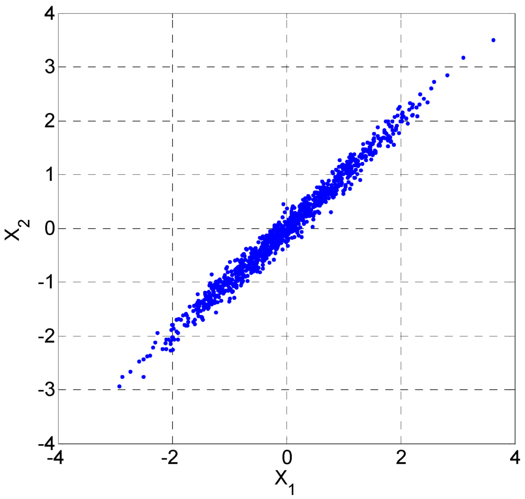
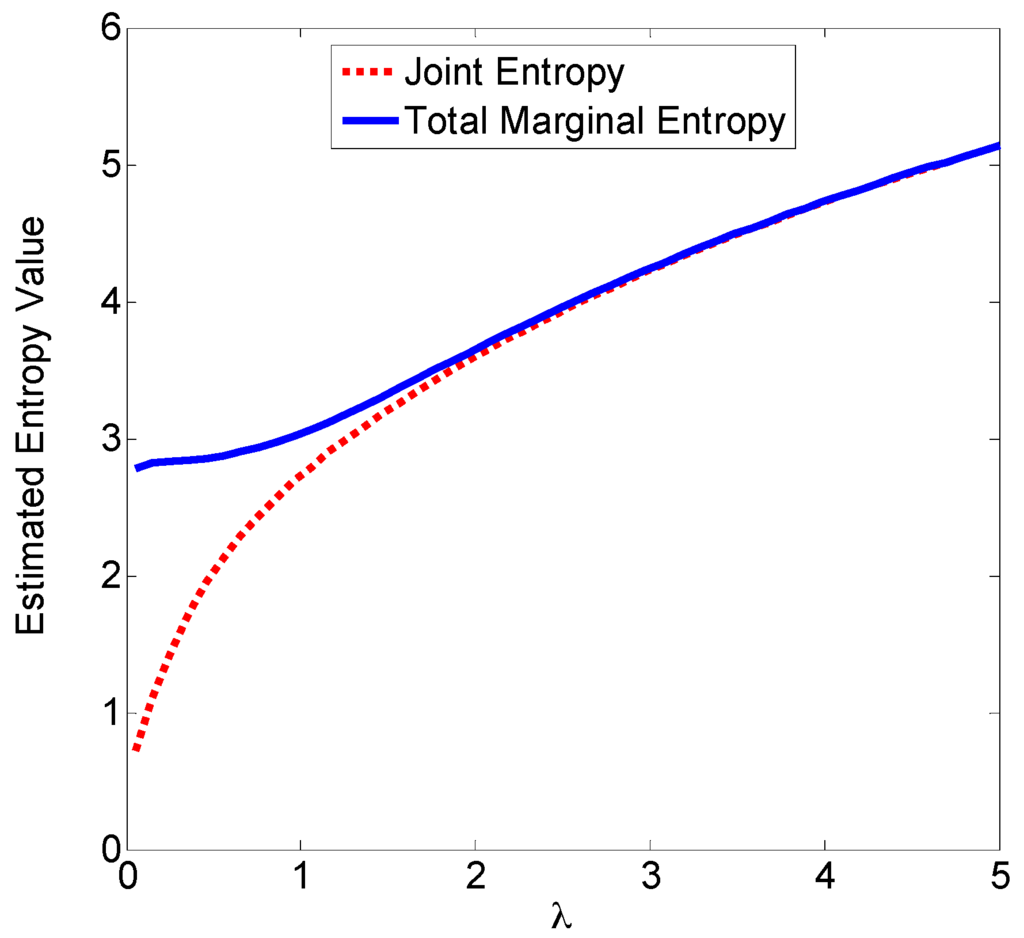
Consider 1000 samples drawn from a two-dimensional Gaussian distribution with zero-mean and covariance matrix ${\Sigma }_X=\left[\begin{array}{cc}1& 0.99\\ 0.99& 1\end{array}\right]$. Figure 2 shows the scatter plot of the samples. Based on these samples, we evaluate the joint entropy and total marginal entropy using Equations (44) and (45), respectively. The estimated entropy values with different $\lambda$ are illustrated in Figure 3, from which we observe that when $\lambda$ becomes larger, the difference between the two estimated entropies will disappear. The results support the Theorem 5.

Figure 2. Scatter plot of the two-dimensional Gaussian samples.

Figure 3. Estimated entropy values with different smoothing factors.

5. Conclusions

Measures of the variability of data play significant roles in many machine learning and signal processing applications. Recent studies suggest that machine learning (supervised or unsupervised) can benefit greatly from the use of entropy as a measure of variability, especially when data possess non-Gaussian distributions. In this paper, we have studied the behaviors of entropy as a measure of multivariate variability. The relationships between multivariate entropy (joint or total marginal) and traditional second-order statistics based multivariate variability measures, such as total dispersion and generalized variance, have been investigated. For the jointly Gaussian case, the joint entropy (or entropy power) is shown to be equivalent to the generalized variance, while total marginal entropy is equivalent to the geometric mean of the marginal variances, and total marginal entropy power is equivalent to the total dispersion. We have also gained insights into the relationships between the smoothed multivariate entropy (joint or total marginal) and the total dispersion. Under certain conditions, the smoothed multivariate entropy will be, approximately, equivalent to the total dispersion. Similar results hold for the multivariate entropy estimators (with finite number of samples) based on the kernel density estimation (KDE). The results of this work can help us to understand the behaviors of multidimensional information theoretic learning.

References

- Cover, T.M.; Thomas, J.A. Elements of Information Theory; Wiley: Hoboken, NJ, USA, 2012. [Google Scholar]
- Renyi, A. On measures of entropy and information. In Proceedings of the Fourth Berkeley Symposium on Mathematical Statistics and Probability, Berkeley, CA, USA, 20 June–30 July 1961; pp. 547–561.
- Tsallis, C. Possible generalization of Boltzmann-Gibbs statistics. J. Stat. Phys. 1988, 52, 479–487. [Google Scholar] [CrossRef]
- Principe, J.C. Information Theoretic Learning: Rényi’s Entropy and Kernel Perspectives; Springer: New York, NY, USA, 2010. [Google Scholar]
- Campbell, L.L. Exponential entropy as a measure of extent of a distribution. Probab. Theory Relat. Fields 1966, 53, 217–225. [Google Scholar] [CrossRef]
- Chen, B.; Zhu, Y.; Hu, J.; Principe, J.C. System Parameter Identification: Information Criteria and Algorithms; Elsevier: Amsterdam, The Netherlands, 2013. [Google Scholar]
- Gokcay, E.; Principe, J.C. Information theoretic clustering. IEEE Trans. Pattern Anal. Mach. Intell. 2002, 24, 158–171. [Google Scholar] [CrossRef]
- Erdogmus, D.; Principe, J.C. From linear adaptive filtering to nonlinear information processing. IEEE Signal Process. Mag. 2006, 23, 15–33. [Google Scholar] [CrossRef]
- Brown, G.; Pocock, A.; Zhao, M.; Luján, M. Conditional likelihood maximization: A unifying framework for information theoretic feature selection. J. Mach. Learn. Res. 2012, 13, 27–66. [Google Scholar]
- Chen, B.; Zhu, P.; Principe, J.C. Survival information potential: A new criterion for adaptive system training. IEEE Trans. Signal Process. 2012, 60, 1184–1194. [Google Scholar] [CrossRef]
- Erdogmus, D.; Principe, J.C. An error-entropy minimization algorithm for supervised training of nonlinear adaptive systems. IEEE Trans. Signal Process. 2002, 50, 1780–1786. [Google Scholar] [CrossRef]
- Erdogmus, D.; Principe, J.C. Generalized information potential criterion for adaptive system training. IEEE Trans. Neural Netw. 2002, 13, 1035–1044. [Google Scholar] [CrossRef] [PubMed]
- Chen, B.; Hu, J.; Pu, L.; Sun, Z. Stochastic gradient algorithm under (h, φ)-entropy criterion. Circuits Syst. Signal Process. 2007, 26, 941–960. [Google Scholar] [CrossRef]
- Chen, B.; Zhu, Y.; Hu, J. Mean-square convergence analysis of ADALINE training with minimum error entropy criterion. IEEE Trans. Neural Netw. 2010, 21, 1168–1179. [Google Scholar] [CrossRef] [PubMed]
- Chen, B.; Principe, J.C. Some further results on the minimum error entropy estimation. Entropy 2012, 14, 966–977. [Google Scholar] [CrossRef]
- Chen, B.; Principe, J.C. On the Smoothed Minimum Error Entropy Criterion. Entropy 2012, 14, 2311–2323. [Google Scholar] [CrossRef]
- Chen, B.; Yuan, Z.; Zheng, N.; Príncipe, J.C. Kernel minimum error entropy algorithm. Neurocomputing 2013, 121, 160–169. [Google Scholar] [CrossRef]
- Kowal, R.R. Note: Disadvantages of the Generalized Variance as a Measure of Variability. Biometrics 1971, 27, 213–216. [Google Scholar] [CrossRef]
- Mustonen, S. A measure for total variability in multivariate normal distribution. Comput. Stat. Data Anal. 1997, 23, 321–334. [Google Scholar] [CrossRef]
- Peña, D.; Rodríguez, J. Descriptive measures of multivariate scatter and linear dependence. J. Multivar. Anal. 2003, 85, 361–374. [Google Scholar] [CrossRef]
- Wilks, S.S. Certain generalizations in the analysis of variance. Biometrika 1932, 24, 471–494. [Google Scholar] [CrossRef]
- Sokal, R.R. Statistical methods in systematics. Biol. Rev. 1965, 40, 337–389. [Google Scholar] [CrossRef] [PubMed]
- Goodman, M. Note: A Measure of “Overall Variability” in Populations. Biometrics 1968, 24, 189–192. [Google Scholar] [CrossRef] [PubMed]
- Barnett, L.; Barrett, A.B.; Seth, A.K. Granger causality and transfer entropy are equivalent for Gaussian variables. Phys. Rev. Lett. 2009, 103, 238701. [Google Scholar] [CrossRef] [PubMed]
- Barrett, A.B.; Barnett, L.; Seth, A.K. Multivariate Granger causality and generalized variance. Phys. Rev. E 2010, 81, 041907. [Google Scholar] [CrossRef] [PubMed]
- Golomb, S. The information generating function of a probability distribution. IEEE Trans. Inf. Theory 1966, 12, 75–77. [Google Scholar] [CrossRef]
- Bobkov, S.; Chistyakov, G.P. Entropy power inequality for the Renyi entropy. IEEE Trans. Inf. Theory 2015, 61, 708–714. [Google Scholar] [CrossRef]
- Kraskov, A.; Stogbauer, H.; Grassberger, P. Estimating Mutual Information. Phys. Rev. E 2004, 69, 066138. [Google Scholar] [CrossRef] [PubMed]
- Silverman, B.W. Density Estimation for Statistics and Data Analysis; Chapman & Hall: New York, NY, USA, 1986. [Google Scholar]
- Rioul, O. Information theoretic proofs of entropy power inequalities. IEEE Trans. Inf. Theory 2011, 57, 33–55. [Google Scholar] [CrossRef]
© 2016 by the authors; licensee MDPI, Basel, Switzerland. This article is an open access article distributed under the terms and conditions of the Creative Commons Attribution (CC-BY) license (http://creativecommons.org/licenses/by/4.0/).