Article

Computational Principle and Performance Evaluation of Coherent Ising Machine Based on Degenerate Optical Parametric Oscillator Network

1
Department of Mathematical Informatics, The University of Tokyo, Hongo 7-3-1, Bunkyo-ku, Tokyo 113-8656, Japan
2
National Institute of Informatics, Hitotsubashi 2-1-2, Chiyoda-ku, Tokyo 101-8403, Japan
3
E. L. Ginzton Laboratory, Stanford University, Stanford, CA 94305, USA
4
ImPACT program, The Japan Science and Technology Agency, Gobancho 7, Chiyoda-ku, Tokyo 102-0076, Japan
*
Author to whom correspondence should be addressed.
Entropy 2016, 18(4), 151; https://doi.org/10.3390/e18040151
Submission received: 20 February 2016 / Revised: 8 April 2016 / Accepted: 12 April 2016 / Published: 19 April 2016

Abstract

:
We present the operational principle of a coherent Ising machine (CIM) based on a degenerate optical parametric oscillator (DOPO) network. A quantum theory of CIM is formulated, and the computational ability of CIM is evaluated by numerical simulation based on c-number stochastic differential equations. We also discuss the advanced CIM with quantum measurement-feedback control and various problems which can be solved by CIM.

1. Introduction

In the field of statistical mechanics, the Ising model describes the simplest mathematical model of spin glass. The model consists of a binary spin system that has the energy called Ising Hamiltonian
H ( σ ) = i < j J i j σ i σ j ( 1 i , j N ) ,
where a real number J i j denotes a coupling constant between every two of the N Ising spins σ i { ± 1 } . To find the minimum energy of the system, i.e., Ising problem, is a well-known combinatorial optimization problem. It generally belongs to the non-deterministic polynomial-time (NP)-hard class in the computational complexity theory, which is believed to be intractable, whereas it can be solved in the polynomial time of the system size N if the spins are aligned in a one-dimensional or two-dimensional lattice with nearest neighbor coupling [1,2]. The problem also attracts broad interest since there are applications in a variety of fields such as computer science [3,4], drug discovery and life-science [5], and information processing technology [6].
Similarly, the goal of a maximum cut problem (MAX-CUT) in the graph theory is to find the size of the largest cut in a given undirected graph G = ( V , E ) . Here, a cut is a partition of the vertices V into two disjoint subsets { S 1 , S 2 } and the size of the cut is defined as the total weight of edges w i j with one vertex i in S 1 and the other j in S 2 . As we assign binary variables σ i { ± 1 } to represent the partition of a vertex V i into two subsets { S 1 , S 2 } , the size of the cut can be counted as follows [1]:
C ( σ ) = i S 1 , j S 2 w i j = i < j w i j ( 1 σ i σ j ) 2 = 1 2 i < j w i j 1 2 H ( σ ) ,
where H is an Ising Hamiltonian defined in Equation (1) with J i j = w i j . It indicates that the MAX-CUT problem is intrinsically equivalent to the Ising problem except for the constant factor.
The MAX-CUT also belongs to the NP-hard class in general, even though there are graph topologies which can be solved in polynomial time of the input [2,7,8,9,10,11]. Many attempts have been made to approximately solve the NP-hard MAX-CUT, but the probabilistically checkable proof (PCP) theorem states that no polynomial time algorithms exist that always find a larger cut than the 0 . 94118 of the optimal solution unless P = NP [12,13]. Currently, the approximation ratio of 0 . 87856 is the best value for performance guarantee, which is achieved by the semidefinite programming (SDP) relaxation algorithm proposed by Goemans and Williamson (GW) [14]. This algorithm is a well-established benchmark target to evaluate any new algorithms or computing methods.
Furthermore, several heuristic algorithms exist to tackle the NP-hard MAX-CUT. The simulated annealing (SA) was designed by mimicking the thermal annealing procedure in metallurgy [15]. A quantum annealing technique was also formulated [16,17,18,19,20] and was shown to have competitive performance against SA. Independently, novel algorithms which are superior either in their speed (the modified version of the Sahni–Gonzalez greedy algorithm (SG3) [21,22]) or its accuracy (named breakout local search (BLS) [23]) are introduced.
We recently proposed a novel computing system to implement the NP-hard Ising problems using the criticality of laser [24,25,26,27] and degenerate optical parametric oscillator (DOPO) phase transition [28,29]. The invention of this machine is motivated by the well-known principle of laser and DOPO in which the mode with a minimum loss rate is most likely to be excited first. The energy of the Ising Hamiltonian can be mapped onto the total loss rate of the laser or DOPO network. The selected oscillation mode in the laser or DOPO network corresponds to the ground state of a given Ising Hamiltonian, while the gain available to all other modes is depleted due to the cross-gain saturation. This means that a mode with the lowest loss rate reaches a threshold condition first and clumps the gain at its loss rate, so that all the other modes with higher loss rates stay at sub-threshold conditions.
This paper is organized as follows. In Section 2, we describe the operational principle of coherent Ising machine (CIM) and present the quantum theory of DOPO network. Section 3 formulates the working equations, c-number stochastic differential equation (CSDE), based on the truncated Wigner distribution function. Then, we conduct numerical simulations for MAX-CUT in Section 4 with the number of vertices up to n = 20 , 000 . We also discuss a practical implementation based on quantum measurement-feedback control and introduce a few problems that can be solved by CIM.

2. Principle

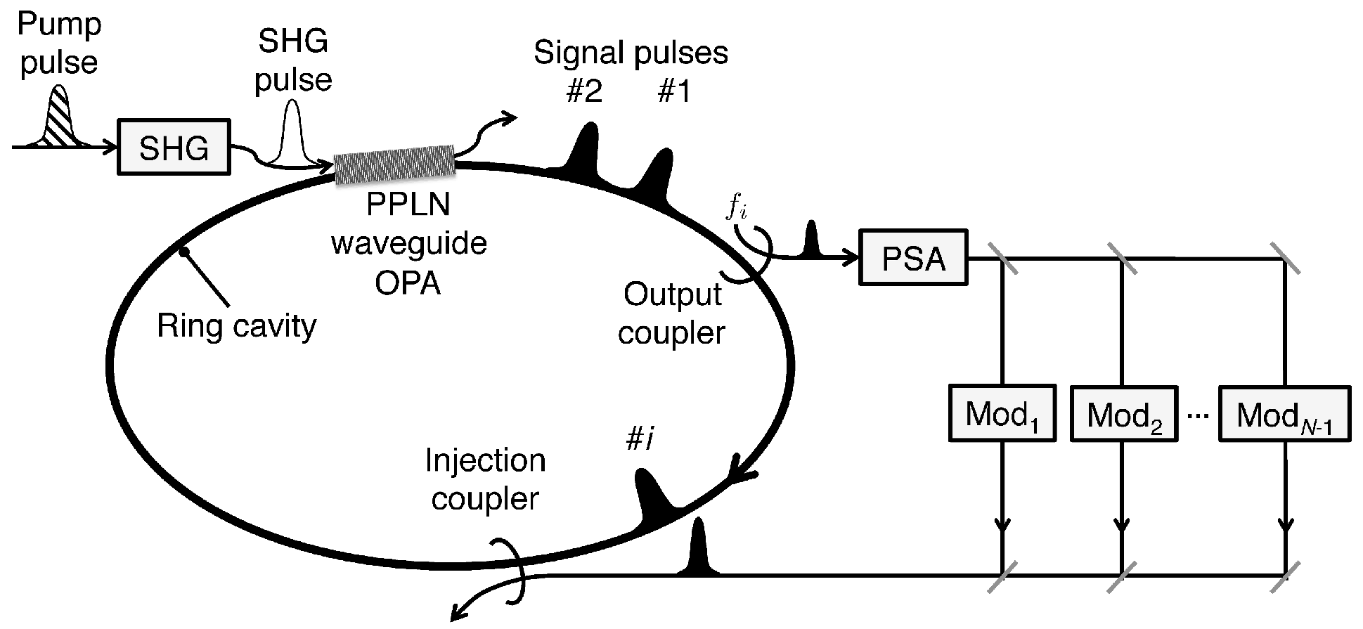
2.1. A Proposed Machine

A CIM based on multiple-pulse DOPO with all-optical mutual coupling is shown in Figure 1. The system starts with a pulsed master laser at a wavelength of 1 . 56 μ m . A second harmonic generation (SHG) crystal produces the pulse train at a wavelength of 0 . 78 μ m , which, in turn, generates multiple DOPO pulses at a wavelength of 1 . 56 μ m inside a fiber ring resonator. If the round trip time of the fiber ring resonator is properly adjusted to N times the pump pulse interval, we can simultaneously generate N independent DOPO pulses inside the resonator. Each of these pulses is either in 0-phase state or π-phase state at well above the oscillation threshold and represents an Ising spin of up or down.
In order to implement an Ising coupling J i j in Equation (1), a part of each DOPO pulse in the fiber ring resonator is picked-off and fed into an optical phase sensitive amplifier (PSA), followed by multiple optical delay lines with intensity and phase modulators. Using such N 1 optical delay lines, (arbitrary) i-th pulse can be coupled to (arbitrary) j-th pulse with a coupling coefficient J i j . Such an all-optical coupling scheme has been demonstrated for N = 4 and N = 16 CIMs in free space [29,30]. In a fiber ring resonator, N = 10 4 CIM with only one-dimensional nearest-neighbor coupling is implemented [31].
In Section 4, we assume the above mentioned CIM with a fiber length of 2 km (or cavity round trip time of 10 μ s) and pulse repetition frequency of 2 GHz (or pulse spacing of 10 cm in the fiber), thus 2 × 10 4 independent DOPO pulses can be prepared for computation on arbitrary graph topology. The system clock frequency for the CIM should be defined by the cavity circulation frequency (inverse of cavity round trip time). One clock cycle (round trip) includes every elements of computation, such as parametric amplification, out-coupling, in-coupling, and fiber delay. Thus, the clock frequency of the CIM assumed for the present benchmark study is 100 kHz since the round trip time of 2 km fiber ring is 10 μ s . We fixed this system clock frequency, just like any digital computer has a fixed clock frequency and chose the appropriate pulse interval to pack the desired number of pulses in the 2 km fiber.

2.2. Quantum Search, Quantum Filtering, and Quantum-to-Classical Crossover

Each DOPO pulse in the coherent Ising machine shown in Figure 1 is in a squeezed vacuum state when a pump rate is well below the oscillation threshold (Figure 2a) and in a (squeezed) coherent state with either 0-phase or π-phase when a pump rate is well above the oscillation threshold (Figure 2b). At the critical point of the DOPO threshold, there exists a linear superposition of the 0-phase and π-phase states [32]. This fact can be easily confirmed by plotting the projection (homodyne) measurement statistics of the quadrature amplitude p ^ = ( a ^ a ^ ) / 2 i at the critical point as shown in Figure 2c. The constructive and destructive interference between the 0-phase and π-phase state is clearly seen when compared to the simple Gaussian distribution [30,33].
Assume without loss of generality N (even number) DOPO pulses have only nearest-neighbor couplings with π-phase shift, and we interpret the 0-phase and π-phase state of each DOPO as Ising spin-up and spin-down states, the coherent Ising machine will find one of the two degenerate ground states in the following four steps.
  • Quantum parallel search
    Each DOPO pulse is in a linear superposition state, but there is no correlation between different DOPO pulses established yet immediately after the pump pulse is switched-on:
    1 2 ( + ) 1 1 2 ( + ) 2 1 2 ( + ) N = 1 2 N ( + + ) .
    However, the probability amplitudes for 2 N spin eigenstates start searching for the ground state of the Ising Hamiltonian via mutual coupling.
  • Quantum filtering
    The probability amplitudes of the two degenerate ground states are amplified, while those of the excited states are deamplified when the pump rate is approaching to the oscillation threshold:
    1 2 ( + ) + ϵ ( all the other states ) ,
    where ϵ > 0 is a small constant. It is numerically founed that such filtering of a quantum entangled state is formed even when the average photon number per DOPO is much smaller than one [34]. A minute energy injected into the system still realized the quantum parallel search and quantum filtering, which promises the success of computation.
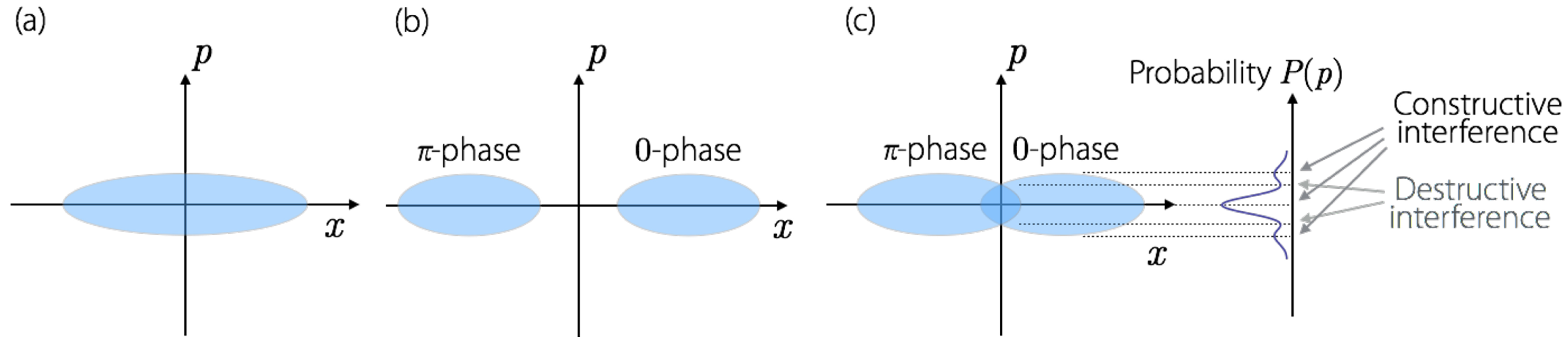
  • Spontaneous symmetry breaking
    At the critical point of the DOPO threshold, random spontaneous emission noise selects one of the two degenerate ground states with equal probabilities. For instance, the probability amplitude of state is amplified but that for the state is deamplified at this stage in one particular run, and vice versa in another run.
  • Quantum-to-classical crossover
    With increasing the pump rate well above the threshold, the chosen spin state dominates over all the other spin states including the other ground state via pump depletion (cross-gain saturation). The quantum state of each DOPO approaches a high excited coherent state with 0-phase or π-phase, which is the closest analog for the classical electromagnetic field.
The four steps of computation in the coherent Ising machine are schematically shown in Figure 3a–d. The CIM starts as a quantum analog computer and ends up as a classical digital computer.

2.3. Quantum Theory of Coherent Ising Machines

The total Hamiltonian of the coherent Ising machine (Figure 1) is
H = H free + H int + H pump + H coupline + H SR ,
H free = ω s j = 1 N a ^ s j a ^ s j + ω p j = 1 N a ^ p j a ^ p j + ω s j = 1 N k j a ^ c j k a ^ c j k ,
H int = i κ 2 j = 1 N ( a ^ s j 2 a ^ p j a ^ p j a ^ s j 2 ) ,
H pump = i j = 1 N ( ε a ^ p j ε a ^ p j ) ,
H couple = i ζ j = 1 k j ( a ^ c j k a ^ s j a ^ c j k a ^ s j + a ^ s k a ^ c j k e i k c z a ^ s k a ^ c j k e i k c z ) ,
H SR = j = 1 N ( a ^ s j Γ ^ Rs j + Γ ^ Rs j a ^ s j + a ^ p j Γ ^ Rp j + Γ ^ Rp j a ^ p j ) + j = 1 N k j ( a ^ c j k Γ ^ Rc + a ^ c j k Γ ^ Rc ) ,
where H free is the free field Hamiltonian for the signal, pump and coupling fields, H int is the parametric interaction Hamiltonian, H pump is the external pumping Hamiltonian where ε is the real-number pump field amplitude, H couple is the coupling Hamiltonian among N DOPOs, H SR is the system-reservoir interaction Hamiltonian which describes any spurious dissipation processes for the signal, pump and coupling fields. In Equation (9), the phase factors of the coupling field represent the in-phase or out-of-phase coupling from the j-th DOPO pulse to the k-th DOPO pulse. The ferromagnetic and anti-ferromagnetic couplings are realized when e i k c z = e i k c z = 1 and e i k c z = e i k c z = 1 , respectively. The two dominating terms in the Hamiltonian are the parametric coupling term H int and the mutual coupling term between different pulses H couple . The former term creates the squeezed vacuum state in each DOPO pulse and makes the quantum parallel search possible, while the latter term modulates the effective loss according to the given problem so that the Ising Hamiltonian is mapped to the network loss.
We can derive the master equation for the total field density operator ρ ^ using Equations (5)–(10) and expand it in terms of the positive-P representation [35]:
ρ ^ = P ( α , β ) α β β * | α d α d β ,
where α = ( α s 1 , , α s N , α p 1 , , α p N , α c 12 , , α c N N 1 ) and β = ( β s 1 , , β s N , β p 1 , , β p N , β c 12 , , β c N N 1 ) are the vectors with complex eigenvalues, α = α s 1 α s N α p 1 α p N α c 12 α c N N 1 and β = β s 1 β s N β p 1 β p N β c 12 β c N N 1 are the multimode coherent states. Here, α X and β X are statistically independent, but their ensemble averaged values satisfy α X = β X * . This off-diagonal α β representation of the field density operator ρ ^ allows to describe an arbitrary non-classical field, while the diagonal α α representation [36] can describe only classical fields or statistical mixture of coherent states. We substitute (11) into the master equation to obtain the Fokker–Planck equation for P ( α , β ) [32]. Then, we can derive the c-number stochastic differential equation (CSDE) using the Ito rule [37]:
d α s k = ( γ s α s k + κ α p k β s k + j k ζ j k α c j k ) d t + κ α p k d w α s k ( t ) ,
d β s k = ( γ s β s k + κ β p k α s k + j k ζ j k β c j k ) d t + κ α p k d w β s k ( t ) ,
d α p k = ( γ p α p k κ 2 α s k 2 + ε ) d t ,
d β p k = ( γ p β p k κ 2 β s k 2 + ε ) d t ,
d α c j k = ( γ c α c j k ζ j k α s j + ζ j k e i θ α s k ) d t ,
d β c j k = ( γ c β c j k ζ j k β s j + ζ j k e i θ β s k ) d t .
The positive-P representation can be obtained by ensemble averaging over many trajectories generated by Monte-Carlo numerical integration of Equations (12)–(17). Typically, we need 10 5 10 6 trajectories for obtaining reasonable convergence. In [33], we demonstrate using the positive-P representation that the two coupled DOPOs feature quantum entanglement and quantum discord in a wide pumping range across the threshold.
It is well-known that even though the positive-P representation method is rigorous and can treat arbitrary non-classical states, the convergence requires a huge computation time. If the quantum state of light in a given physical system is only slightly deviated from the Gaussian states, the truncated Wigner representation is an alternative approach with reasonable accuracy [37]. In this case, the field density operator is expanded by the Wigner function W ( α ) :
ρ ^ = e λ * a ^ λ a ^ e λ a * λ * a W ( α ) d α d λ ,
where a ^ = ( a ^ s 1 , , a ^ s N , a ^ p 1 , , a ^ p N , a ^ c 12 , , a ^ c N N 1 ) and λ = ( λ s 1 , , λ s N , λ p 1 , , λ p N , λ c 12 , , λ c N N 1 ) . χ ( λ ) = e λ a * λ * a W ( α ) d α is the symmetric correlation function. W ( α ) and χ ( λ ) form a pair of Fourier transform. The Fokker–Planck equation for W ( α ) can be derived by truncating the third and higher-order terms, which gives another set of CSDEs:
d α s k = ( γ s α s k + κ α p k α s k * + j k ζ j k α c j k ) d t + γ s d W s k ( t ) ,
d α p k = ( γ p α p k κ 2 α s k 2 + ε ) d t + γ p d W p k ( t ) ,
d α c j k = ( γ c α c j k ζ j k α s j + ζ j k e i θ α s k ) d t + γ c d W c k ( t ) .
Here, d W X ( t ) is the c-number Wiener process and corresponds to the quantum noise injected into the system from external reservoirs. In [34], we demonstrate the degree of quantum entanglement predicted by the positive-P representation method and the truncated Wigner function method agree with each other within the statistical error introduced by the finite number of numerically generated trajectories in the case of N = 2 and N = 16 .
If we are only interested in the final destination of each DOPO, that is, either 0-phase or π-phase coherent state at well above the threshold, we do not need to reconstruct the density operator at all time. Instead, we can read out the polarity of the real part of the c-number eigenvalue, Re ( α s k ) , to determine the computational result: Re ( α s k ) > 0 k or Re ( α s k ) < 0 k . This means that if we run the Monte-Carlo numerical integration of Equations (19)–(21) over 10 3 times, we can obtain the success/failure statistics of 10 3 independent computation sessions. This is exactly the numerical method we use in this paper.

3. Working Equations

3.1. c-Number Stochastic Differential Equations for Multiple-Pulse DOPO with Mutual Coupling

The in-phase and quadrature-phase amplitudes of a single isolated DOPO pulse obey the following c-number stochastic differential equations (CSDE) [34,38]:
d c = ( 1 + p c 2 s 2 ) c d t + 1 A s c 2 + s 2 + 1 2 d W 1 ,
d s = ( 1 p c 2 s 2 ) s d t + 1 A s c 2 + s 2 + 1 2 d W 2 .
The pump field is adiabatically eliminated in Equations (22) and (23) by assuming that the pump photon decay rate γ p is much larger than the signal photon decay rate γ s . The saturation amplitude A s = ( γ s γ p / 2 κ 2 ) 1 / 2 is the DOPO field amplitude at a normalized pump rate p = F p / F th = 2 , and κ is the second order nonlinear coefficient associated with the degenerate optical parametric amplification. The variable t = γ s τ / 2 is a normalized time, while τ is a real time in seconds. The term F p is the pump field amplitude and F th = γ s γ p / 4 κ is the threshold pump field amplitude. Finally, d W 1 and d W 2 are two independent Gaussian noise processes that represent the incident vacuum fluctuations from the open port of the output coupler and the pump field fluctuation for in-phase and quadrature-phase components, respectively. The vacuum fluctuation of the signal channel contributes to the 1/2 term, and the quantum noise of the pump field contributes to c 2 + s 2 in the square-root bracket in Equations (22) and (23).
When the i-th signal pulse is incident upon the output coupler, the out-coupled field is normalized to the inferred signal:
c ˜ i c i , out T = c i 1 T T f i A s ,
where T is the power transmission coefficient of the output coupler and f i is the incident vacuum fluctuation from the open port of the coupler. These out-coupled pulses are divided into N 1 delay lines with intensity and pahse modulators placed in each delay path as shown in Figure 1, and produce the mutual coupling optical pulse j ξ i j c ˜ j , which is actually added to the i-th signal pulse by an injection coupler. Here, ξ i j is the effective coupling coefficient from the j-th pulse to the i-th pulse, determined by the transmission coefficient T of the injection coupler. In the highly dissipative limit of a mutual coupling circuit, we can use the CSDE supplemented with the noisy coupling term. Since we assume the transmission coefficient T of the injection coupler is much smaller than one, any additional noise in the injected feedback pulse can be neglected. The CSDE (22) can be now rewritten to include the mutual coupling terms
d c i = [ ( 1 + p c i 2 s i 2 ) c i + j ξ i j c ˜ j ] d t + 1 A s c i 2 + s i 2 + 1 2 d W i .
The summation in Equation (25) represents the feedback term including the vacuum fluctuation given by Equation (24). We conducted the numerical simulation of the coupled CSDE (25) to evaluate the performance of the CIM. Figure 4 shows typical trajectories of DOPO amplitudes after the pump pulses are switched-on at t = 0 . It is shown that most of DOPO pulses reach the steady state after 20 to 30 round trips, while a few of others need 100 round trips to reach the steady state.

3.2. Turn-on Delay Time

The computation time of a CIM is governed by the time for each DOPO to reach the steady state after the pump power is switched on. We consider the simplest case such that all DOPOs have identical amplitudes except their phases and complete mutual coupling without frustration. In this case, the CSDE is simplified as
d d t c = [ 1 + p c 2 + ( N 1 ) ξ ] c + 1 A s c 2 + 1 2 d W 1 .
When the pump power is switched on but the field is still less than the steady state value, we can neglect the non-linear saturation term of the above equation. Thus, the DOPO field increases exponentially as
c ( t ) = c ( 0 ) exp { [ p 1 + ( N 1 ) ξ ] t } ,
where c ( 0 ) is the initial amplitude governed by the vacuum fluctuation. At the steady state condition, the signal field is given by c ( t ) = p 1 + ( N 1 ) ξ , so that the normalized time to reach the steady state amplitude is given by
t turn on = log [ p 1 + ( N 1 ) ξ A s ] p 1 + ( N 1 ) ξ ,
where c ( 0 ) O ( 1 / A s ) is used. The turn-on delay time is shortened by increasing the pump rate p and the coupling constant ξ and by decreasing the signal photon lifetime and the saturation amplitude A s . When the mutual coupling has the frustration like the case of Figure 4, the coupling factor ( N 1 ) ξ in Equation (28) is reduced to ξ in the most frustrated spin.

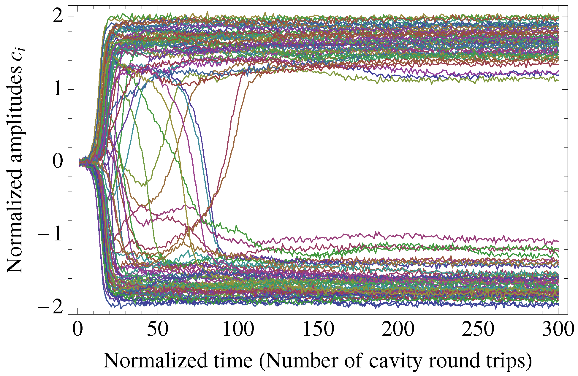
4. Numerical Simulations

The performance of the CIM are evaluated for MAX-CUT in comparison with representative approximation algorithms mentioned in the Introduction. Here, computational experiments were conducted on fully connected complete graphs, denoted by K n , where the number of vertices n ranging from 40 to 20,000 and the n ( n 1 ) /2 edges are randomly weighted { ± 1 } . We need N = n DOPO pulses in a fiber ring resonator.
Since the MAX-CUT is NP-hard and it is difficult to measure the time to the optimal solution for such a large problem size, the GW solution was used as the mark of sufficient accuracy because it ensures better than the 87.856% of the ground states. The CIM and other approximation algorithms are compared in terms of computation time to reach the same values obtained by GW. Note that the number of spin flipping for the SA was optimized with the inverse temperature scheduling of logarithmic function.
The algorithms are coded in C/C++ and run on a single thread of a single core on a Linux machine with two 6-core Intel Xeon X5650 (2.67 GHz) processors and 94 GB RAM. The computational process of CIM is simulated based on the coupled CSDE (25) on the same machine. Note that the computation time of CIM does not mean the simulation time took on the Linux machine but means the actual evolution time of a physical CIM.
Table 1 shows the computation time versus problem size (number of vertices). The computation time is defined as the CPU time to reach the number of cuts a given MAX-CUT on complete graph by GW; as the CPU time to reach the same accuracy as GW for SA, SG3, and BLS; and as the time estimated by the (number of round trips) × (cavity round trip time) to obtain the same accuracy as GW for CIM. The preparation time needed to input J i j into the computing system, i.e., the graph I/O time, is not included. For complete graphs of n 20 , 000 , the CIM exhibits a problem-size independent computation time of less than 10 3 s if we assume the fixed cavity circulation frequency (clock frequency) of 100 kHz and pulse interval of 10 cm. This means the target accuracy is obtained in the constant number of round trips. It indicate that the computation time of CIM is determined by the turn-on delay time Equation (28) of the DOPO network oscillation, which in turn depends on the round trip time and the pump rate.
The time complexity O ( n 3 . 5 ) for the GW is dominated by the interior-point method in the Goemans–Williamson algorithm. The SA seems to scale in O ( n 2 ) , which indicates that it requires the number of spin flips to be proportional to n (i.e., constant Monte Carlo steps) to achieve the optimal performance. Each spin flip costs a computation time proportional to the degree k i , where k i is equal to n 1 for all i V in the case of complete graphs. Thus, the computation time scales as O ( n k ) = O ( n 2 ) for the SA in the complete graphs. Note that CIM and SA did not always reach the energy obtained by GW for the graph of n = 40 , half of the 100 runs of stochastic algorithms were post-selected to reach that value. SG3 is expected to scales as O ( m ) = O ( n 2 ) , but in the table, values for n = 40 , 160 , 800 are not shown because it didn’t reach the accuracy reached by the GW solution. BLS exhibits competitive performance against SA.
Note that those numerical results come from a specific computer configuration as mentioned above. Thus, there is room for an improvement in the computation time in constant factor due to cases like using faster CPUs or parallelized codes. Similarly, the computation time of CIM also depends on the system configuration and can be made faster when we use the higher clock frequency. In this sense, the ratios between time of CIM and that of the other algorithms are arbitrary. Thus, we should study the computation time scaling as a function of the problem size.
In Table 2, the computation times of the CIM with different fiber length and pulse repetition frequency are shown (see the Section 2.1 for the definition). Since the solutions are obtained in a constant number of cavity round trips, the computation time is repetition frequency independent but linearly depends on the cavity length of the fiber. The system clock frequency is determined by the circulation time of 10 μ s around 2 km fiber ring cavity and is equal to 100 kHz. The computation time of CIM is governed by this clock frequency of 100 kHz. The number of pulses accommodated in the fiber can be changed to vary the pulse repetition frequency under the fixed fiber length. On the other hand, when the pulse repetition frequency is fixed and the fiber length is varied, the maximum number of pulses should be increased in proportional to the fiber length. Note though the phase stabilization in the fiber length of 20 km is challenging and the 200 GHz repetition frequency is not yet practically available, we do not think it is impractical in the near future.

5. Discussion

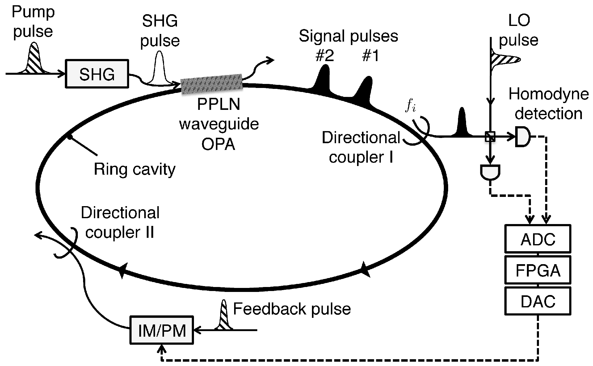
5.1. Measurement-Feedback Control

When we wish to build a large-scale experimental system of CIM, one serious problem is how to stabilize all optical delay lines for mutual injection paths. An alternative way is quantum measurement-based mutual coupling scheme, which is shown in Figure 5. A fiber ring resonator is composed of three components: an optical parametric amplifier and two directional couplers. These directional couplers I and II are used as an out-coupling port to the optical homodyne detectors and feedback signal injecting port for providing the mutual coupling between the DOPO pulses, respectively. Instead of directly connecting the DOPO pulses with optical delay lines, we can measure the in-phase amplitude c ˜ j of the j-th pulse and compute the proper feedback pulse amplitude for the i-th pulse j ξ i j c ˜ j by the digital electronic circuit, where the coupling coefficient ξ i j is proportional to the Ising coupling J i j . The output electrical signal drives the intensity and phase modulators to properly generate a feedback pulse for the i-th pulse. To synchronously calculate this matrix-vector product in each cavity round trip, a field programmable gate array (FPGA) or application specific integrated circuit (ASIC) can be installed. Such a hybrid optoelectronic coupling scheme is equivalent to the purely optical coupling scheme except for the small difference in noise penalty.
A clear advantage of the hybrid optoelectronic coupling scheme is that all the Ising coupling J i j of the order of N 2 can be implemented by a single quantum measurement-feedback control circuit. In addition, the multi-body interactions, such as H = ξ i j k σ i σ j σ k , can be readily implemented with the measurement-feedback control. For example, a current high-performance FPGA has about 10 6 multiplier units, hence two FPGAs can accommodate the full adjacency matrix of N = 2000 graph which has 2 × 10 6 elements. In order to implement larger graphs, multiple high-end FPGAs should be stacked to process O ( N 2 ) multiplication per each round trip. On the other hand, all optical coupling scheme enjoys its inherent high-speed operation, even though it requires N 1 optical delay lines.

5.2. Application to Various Problems

The objective functions of many optimization problems can be mapped to the Ising problem. Here, the Ising problem, MAX-CUT and quadratic unconstrained binary optimization (QUBO) are intrinsically equivalent. The former two problems are { + 1 , 1 } -valued optimization and the latter is a { 0 , 1 } -valued optimization, whose variables σ { ± 1 } and x { 0 , 1 } are mutually convertible with x = ( 1 + σ ) / 2 . Hence, the mapping to QUBO is sufficient which has an Ising-type cost function:
H QUBO = i < j Q i j x i x j ,
where Q i j is a coupling constant.
We will see a 3-SAT problem as an example of the mapping. The boolean satisfiability problem (SAT) is a problem to find a correct variable assignment which satisfies a given conjunctive normal form (CNF) S with n variables and m clauses. 3-SAT is a subset of this problem, in which we are asked the satisfiability of clauses C i ( i = 1 , , m ) each containing exactly 3 literals X 1 ( i ) , X 2 ( i ) , X 3 ( i ) , and each literal X j ( i ) is a variable x k or its complement x ¯ k :
S = i = 1 , , m j = 1 , 2 , 3 X j ( i ) , where X j ( i ) k = 1 , , n { x k , x ¯ k } .
There are three ways to map the 3-SAT to Ising problem.
  • Via MAX-2-SAT
    MAX-2-SAT is a problem to find an assignment for a given 2-CNF which satisfies as many clauses as possible. We can construct a CNF of MAX-2-SAT S ˜ from a given 3-CNF S with using an auxiliary literal Y ( i ) for each clause C i = X 1 ( i ) X 2 ( i ) X 3 ( i ) [1]:
    S ˜ = i = 1 , , m D i ,
    where
    D i = X 1 ( i ) X 2 ( i ) X 3 ( i ) Y ( i ) ( ¬ X 1 ( i ) ¬ X 2 ( i ) ) ( ¬ X 2 ( i ) ¬ X 3 ( i ) ) ( ¬ X 3 ( i ) ¬ X 1 ( i ) ) ( X 1 ( i ) ¬ Y ( i ) ) ( X 2 ( i ) ¬ Y ( i ) ) ( X 3 ( i ) ¬ Y ( i ) ) .
    For each D i , we can satisfy exactly seven within 10 clauses if the original C i is satisfiable. If not, the satisfiable clauses in D i is six. Hence, 7 m within 10 m clauses in S ˜ can be satisfied simultaneously if and only if the given CNF S is satisfiable. The 3-SAT became a MAX-2-SAT with n + m variables and 10 m clauses. Then, it is easily converted to QUBO as replacing the literal X j to a variable x j , the negation of literal ¬ X j to ( 1 x j ) , respectively ( j = 1 , , m + n ) , and the clauses to AND operation of variables [40]:
    H QUBO = i = 1 m { 4 x 1 ( i ) x 2 ( i ) x 3 ( i ) + 2 y 1 ( i ) + x 1 ( i ) x 2 ( i ) + x 2 ( i ) x 3 ( i ) + x 3 ( i ) x 1 ( i ) x 1 ( i ) y ( i ) x 2 ( i ) y ( i ) x 3 ( i ) y ( i ) } ,
    whose ground state energy is 3 m if and only if it is satisfiable.
  • Via Maximum independent set (MIS)
    3-SAT can be described in terms of MIS on a graph with 3 m vertices. The graph can be constructed to connect the contradicting literals in m triangle graphs (each triangle graph represent a clause). Then there exist independent sets of size m, if and only if the original 3-CNF is satisfiable. Since the MIS is mapped to an Ising problem with the equivalent number of vertices [41], 3-SAT becomes 3 m -spin Ising problem in this case. The Ising coupling term takes only J i j { 0 , ± 1 } in this case.
  • Via 3-body problem
    3-SAT is easily interpreted as an optimization problem which has cost function with up to 3-body interactions
    H ( i ) = J 1 ( i ) x 1 ( i ) J 2 ( i ) x 2 ( i ) J 1 ( i ) x 3 ( i ) + J 12 ( i ) x 1 ( i ) x 2 ( i ) + J 23 ( i ) x 2 ( i ) x 3 ( i ) + J 31 ( i ) x 3 ( i ) x 1 ( i ) J 123 ( i ) x 1 ( i ) x 2 ( i ) x 3 ( i ) ,
    where the coefficients J j ( i ) , J j 1 j 2 ( i ) , J 123 ( i ) ( j , j 1 , j 2 { 1 , 2 , 3 } ) are given from literals in 3-CNF
    J j ( i ) = 1 if X j ( i ) = x k , 0 if X j ( i ) = x ¯ k ,
    J j 1 j 2 ( i ) = J j 1 ( i ) J j 2 ( i ) ,
    J 123 ( i ) = J 1 ( i ) J 2 ( i ) J 3 ( i ) ,
    and x j ( i ) { 0 , 1 } represent boolean values. To replace the 3-body term x 1 ( i ) x 2 ( i ) x 3 ( i ) with the 2-body interaction, we introduce an auxiliary spin y ( i ) , which keeps y ( i ) = x 1 ( i ) x 2 ( i ) with the penalty term E p ( i ) [42]:
    E p ( i ) = b ( 3 y ( i ) + x 1 ( i ) x 2 ( i ) 2 y ( i ) x 1 ( i ) 2 y ( i ) x 2 ( i ) ) ,
    where b > 1 is a penalty strength. Then, the summation of
    H QUBO ( i ) = J 1 ( i ) x 1 ( i ) J 2 ( i ) x 2 ( i ) J 1 ( i ) x 3 ( i ) + J 12 ( i ) x 1 ( i ) x 2 ( i ) + J 23 ( i ) x 2 ( i ) x 3 ( i ) + J 31 ( i ) x 3 ( i ) x 1 ( i ) J 123 ( i ) y ( i ) x 3 ( i ) + E p ( i ) ,
    over i = 1 , , m gives the 2-body Hamiltonian with the ground state of energy 0.
There are other problems which can be mapped to Ising problems other than 3-SAT, which are summarized in Table 3 (see also [41]). Note that the required number of DOPO pulses N is proportional to the graph order n, except for TSP and Hamiltonian path problems.

6. Conclusions

In this paper, we presented the physical implementation and operational principle of a CIM. When it explores the solution space, it utilizes the linear superposition state and quantum entanglement. The quantum mechanical model and the numerical method are described.
The potential for solving NP-hard problems using a CIM was numerically studied against existing approximation algorithms. The computational experiments are conducted for the MAX-CUT on fully connected complete graphs up to N = 2 × 10 4 . The results imply that the CIM achieves empirically constant time scaling in a fixed system clock frequency, i.e., the fixed cavity circulation frequency (fiber length), while the SA, SG3, and BLS scale as O ( N 2 ) and GW scales as O ( N 3 . 5 ) . Those results suggest that CIM may find applications in high-speed computation for various combinatorial optimization problems.
We also discussed the practical implementation and a few applications. The measurement-feedback based CIM is the most promising way to implement large-sized problems with dense and arbitrary random connections between vertices. The present simulation results do not mean that the CIM can get a reasonably accurate solution by a constant time for arbitrary large problem size. As mentioned already, in the CIM based on a fiber ring resonator, the number of DOPO pulses is determined by the the fiber length and the pulse spacing. In order to implement 2 × 10 5 and 2 × 10 6 DOPO pulses in the 20 km fiber ring cavity, we must use a pulse repetition frequency to 2 GHz and 20 GHz, respectively. In addition, we must install a measurement-feedback system which can handle the connectivity of the given graph. This is certainly within reach in current advanced technologies.

Acknowledgments

The authors would like to thank K. Kawarabayashi, M. Oku, K. Aihara, K. Inoue, H. Takesue, A. Marandi, P. McMahon, K. Igarashi, T. Inagaki, T. Leleu, S. Tamate, Z. Wang, K. Takata, H. Sakaguchi, and D. Maruo for their useful discussions. This project is supported by the ImPACT program of the Japanese Cabinet Office.

Author Contributions

Yoshitaka Haribara, Shoko Utsunomiya and Yoshihisa Yamamoto conceived and designed the study; Yoshitaka Haribara performed the numerical experiments; Yoshitaka Haribara, Shoko Utsunomiya and Yoshihisa Yamamoto wrote the paper. All authors have read and approved the final manuscript.

Conflicts of Interest

The authors declare no conflict of interest.

Abbreviations

The following abbreviations are used in this manuscript:
CIM
Coherent Ising machine
DOPO
Degenerate optical parametric oscillator
NP
Non-deterministic polynomial-time
MAX-CUT
Maximum cut problem
GW
Goemans–Williamson
SA
Simulated annealing
SG
Sahni–Gonzalez
BLS
Breakout local search
CSDE
c-number stochastic differential equation
SHG
Second harmonic generation
PSA
Phase sensitive amplifier
FPGA
Field programmable gate array
ASIC
Application specific integrated circuit
QUBO
Quadratic unconstrained binary optimization
SAT
Boolean satisfiability problem
CNF
Conjunctive normal form
MIS
Maximum independent set
TSP
Traveling salesman problem

References

  1. Garey, M.R.; Johnson, D.S. Computers and Intractability: A Guide to the Theory of NP-Completeness; Freeman: San Francisco, CA, USA, 1979. [Google Scholar]
  2. Barahona, F.J. On the computational complexity of Ising spin glass models. Phys. A 1982, 15, 3241–3253. [Google Scholar] [CrossRef]
  3. Karp, R.M. Complexity of Computer Computations; Millera, R.E., Thatcher, J.W., Eds.; Plenum: New York, NY, USA, 1972; pp. 85–103. [Google Scholar]
  4. Mézard, M.; Parisi, G.; Virasoro, M. Spin Glass Theory and Beyond; World Scientific: Singapore, Singapore, 1987. [Google Scholar]
  5. Kitchen, D.B.; Decornez, H.; Furr, J.R.; Bajorath, J. Docking and scoring in virtual screening for drug discovery: Methods and applications. Nat. Rev. Drug Discov. 2004, 3, 935–949. [Google Scholar] [CrossRef] [PubMed]
  6. Nishimori, H. Statistical Physics of Spin Glasses and Information Processing; Oxford University Press: Oxford, UK, 2001. [Google Scholar]
  7. Orlova, G.I.; Dorfman, Y.G. Finding the maximum cut in a graph. Eng. Cybern. 1972, 10, 502–506. [Google Scholar]
  8. Hadlock, F. Finding a Maximum Cut of a Planar Graph in Polynomial Time. SIAM J. Comput. 1975, 4, 221–225. [Google Scholar] [CrossRef]
  9. Grötschel, M.; Pulleyblank, W.R. Weakly bipartite graphs and the Max-cut problem. Oper. Res. Lett. 1981, 1, 23–27. [Google Scholar] [CrossRef]
  10. Grötschel, M.; Nemhauser, G.L. A polynomial algorithm for the max-cut problem on graphs without long odd cycles. Math. Program. 1984, 29, 28–40. [Google Scholar] [CrossRef]
  11. Galluccio, A.; Loebl, M.; Vondrák, J. Optimization via enumeration: A new algorithm for the Max Cut Problem. Math. Program. 2001, 90, 273–290. [Google Scholar] [CrossRef]
  12. Arora, S.; Lund, C.; Motwani, R.; Sudan, M.; Szegedy, M. Proof verification and the hardness of approximation problems. J. ACM 1998, 45, 501–555. [Google Scholar] [CrossRef]
  13. Håstad, J. Some optimal inapproximability results. J. ACM 2001, 48, 798–859. [Google Scholar] [CrossRef]
  14. Goemans, M.X.; Williamson, D.P. Improved approximation algorithms for maximum cut and satisfiability problems using semidefinite programming. J. ACM 1995, 42, 1115–1145. [Google Scholar] [CrossRef]
  15. Kirkpatrick, S.; Gelatt, C.D., Jr.; Vecchi, M.P. Optimization by Simulated Annealing. Science 1983, 220, 671–680. [Google Scholar] [CrossRef] [PubMed]
  16. Kadowaki, T.; Nishimori, H. Quantum annealing in the transverse Ising model. Phys. Rev. E 1998, 58, 5355–5363. [Google Scholar] [CrossRef]
  17. Santoro, G.E.; Martoňák, R.; Tosatti, E.; Car, R. Theory of Quantum Annealing of an Ising Spin Glass. Science 2002, 295, 2427–2430. [Google Scholar] [CrossRef] [PubMed]
  18. Farhi, E.; Goldstone, J.; Gutmann, S.; Lapan, J.; Lundgren, A.; Preda, D. A Quantum Adiabatic Evolution Algorithm Applied to Random Instances of an NP-Complete Problem. Science 2001, 292, 472–475. [Google Scholar] [CrossRef] [PubMed]
  19. Van Dam, W.; Mosca, M.; Vazirani, U.V. How powerful is adiabatic quantum computation? In Proceedings of the 42nd IEEE Symposium on Foundations of Computer Science; IEEE Computer Society: Los Alamitos, CA, USA, 2001; pp. 279–287. [Google Scholar]
  20. Aharonov, D.; van Dam, W.; Kempe, J.; Landau, Z.; Lloyd, S.; Regev, O. Adiabatic Quantum Computation Is Equivalent to Standard Quantum Computation. SIAM J. Comput. 2008, 50, 755–787. [Google Scholar] [CrossRef]
  21. Sahni, S.; Gonzalez, T. P-Complete Approximation Problems. J. ACM 1976, 23, 555–565. [Google Scholar] [CrossRef]
  22. Kahruman, S.; Kolotoglu, E.; Butenko, S.; Hicks, I.V. On greedy construction heuristics for the MAX-CUT problem. Int. J. Comput. Sci. Eng. 2007, 3, 211–218. [Google Scholar] [CrossRef]
  23. Benlic, U.; Hao, J.-K. Breakout Local Search for the Max-Cutproblem. Eng. Appl. Artif. Intel. 2013, 26, 1162–1173. [Google Scholar] [CrossRef] [Green Version]
  24. Utsunomiya, S.; Takata, K.; Yamamoto, Y. Mapping of Ising models onto injection-locked laser systems. Opt. Express 2011, 19, 18091–18108. [Google Scholar] [CrossRef] [PubMed]
  25. Takata, K.; Utsunomiya, S.; Yamamoto, Y. Transient time of an Ising machine based on injection-locked laser network. New J. Phys. 2012, 14, 013052–013073. [Google Scholar] [CrossRef]
  26. Takata, K.; Yamamoto, Y. Data search by a coherent Ising machine based on an injection-locked laser network with gradual pumping or coupling. Phys. Rev. A 2014, 89, 032319. [Google Scholar] [CrossRef]
  27. Utsunomiya, S.; Namekata, N.; Takata, K.; Akamatsu, D.; Inoue, S.; Yamamoto, Y. Binary phase oscillation of two mutually coupled semiconductor lasers. Opt. Express 2015, 23, 6029–6040. [Google Scholar] [CrossRef] [PubMed]
  28. Wang, Z.; Marandi, A.; Wen, K.; Byer, R.L.; Yamamoto, Y. Coherent Ising machine based on degenerate optical parametric oscillators. Phys. Rev. A 2013, 88, 063853. [Google Scholar] [CrossRef]
  29. Marandi, A.; Wang, Z.; Takata, K.; Byer, R.L.; Yamamoto, Y. Network of time-multiplexed optical parametric oscillators as a coherent Ising machine. Nat. Photon. 2014, 8, 937–942. [Google Scholar] [CrossRef]
  30. Takata, K. Quantum theory and Experimental Demonstration of a Coherent Computing System with Optical Parametric Oscillators. Ph.D. Thesis, the University of Tokyo, Tokyo, Japan, 2015. [Google Scholar]
  31. Inagaki, T. Large-scale Ising spin network based on degenerate optical parametric oscillator. Nat. Phys. 2016, in press. [Google Scholar]
  32. Drummond, P.D.; Gardiner, C.W.J. Generalised P-representations in quantum optics. Phys. A 1980, 13, 2353–2368. [Google Scholar] [CrossRef]
  33. Takata, K.; Marandi, A.; Yamamoto, Y. Quantum correlation in degenerate optical parametric oscillators with mutual injections. Phys. Rev. A 2015, 92, 043821. [Google Scholar] [CrossRef]
  34. Maruo, D.; Utsunomiya, S.; Yamamoto, Y. Truncated Wigner theory of coherent Ising machines based on degenerate optical parametric oscillator network. Phys. Scripta 2016, in press. [Google Scholar]
  35. Drummond, P.D.; McNeil, K.J.; Walls, D.F. Non-equilibrium Transitions in Sub/Second Harmonic Generation II. Quantum theory. Opt. Acta 1981, 28, 211–225. [Google Scholar] [CrossRef]
  36. Glauber, R.J. Coherent and Incoherent States of the Radiation Field. Phys. Rev. 1963, 131. [Google Scholar] [CrossRef]
  37. Carmichael, H. Statistical Methods in Quantum Optics 1: Master Equations and Fokker-Planck Equations; Springer: Berlin, Germany, 1999. [Google Scholar]
  38. Kinsler, P.; Drummond, P.D. Quantum dynamics of the parametric oscillator. Phys. Rev. A 1991, 43, 6194–6208. [Google Scholar] [CrossRef]
  39. Haribara, Y.; Utsunomiya, S.; Kawarabayashi, K.; Yamamoto, Y. Encyclopedia of Spectroscopy and Spectrometry, 3rd ed.; Elsevier: Oxford, UK, 2016. [Google Scholar]
  40. Santra, S.; Quiroz, G.; Steeg, G.V.; Lidar, D.A. Dynamically probing ultracold lattice gases via Rydberg molecules. New J. Phys. 2015, 17, 103024. [Google Scholar]
  41. Lucas, A. Ising formulations of many NP problems. Front. Phys. 2014, 2, 5. [Google Scholar] [CrossRef]
  42. Perdomo-Ortiz, A.; Dickson, N.; Drew-Brook, M.; Rose, G.; Aspuru-Guzik, A. Finding low-energy conformations of lattice protein models by quantum annealing. Sci. Rep. 2012, 2. [Google Scholar] [CrossRef] [PubMed]
Figure 1. A coherent Ising machine based on the time-division multiplexed DOPO with mutual coupling implemented by optical delay lines. A part of each pulse is picked off from the main cavity by the output coupler followed by an optical phase sensitive amplifier (PSA) which amplifies the in-phase amplitude c ˜ i of each DOPO pulse. The feedback pulses, which are produced by combining the outputs from N 1 intensity and phase modulators, are injected back to the main cavity by the injection coupler.
Entropy 18 00151 g001
Figure 2. Quantum states of a DOPO at (a) below; (b) above; and (c) critical point of its oscillation threshold.
Entropy 18 00151 g002
Figure 3. Four steps of computation in a coherent Ising machine: (a) quantum parallel search; (b) quantum filtering; (c) spontaneous symmetry breaking; and (d) quantum-to-classical crossover.
Entropy 18 00151 g003
Figure 4. Normalized DOPO signal amplitudes when CIM is solving N = 800 MAX-CUT is shown. Each trajectory describes a DOPO.
Entropy 18 00151 g004
Figure 5. Quantum measurement-feedback controlled CIM. Small portion of each signal pulse is out-coupled through the directional coupler I, and its in-phase component is measured by optical balanced homodyne detector, where LO pulse is directly obtained from the master laser. Two detector outputs are converted to digital signals and input into an electronic digital circuit, where a feedback signal for i-th signal pulse is computed. Independently obtained feedback pulse from the master laser is modulated in its intensity and phase to achieve j ξ i j c ˜ j and coupled into i-th signal pulse by directional coupler II. Flows of optical fields and electrical signals are shown as solid and dashed lines, respectively.
Entropy 18 00151 g005
Table 1. Computation time (sec.) on { ± 1 } -weighted complete graphs. The symbol “–” means it didn’t reach the desired accuracy (see also [39]).
Method/AlgorithmGraph Order n ( = N )
40160800400020,000
GW0.003450.17022.5 6 . 65 × 10 3 1 . 81 × 10 6
SA0.009060.0201.3010.2210
BLS 7 . 92 × 10 4 0.02550.04651.2252.3
SG30.59215.3
CIM0.002970.002560.000400.000550.00199
Table 2. Fiber length and pulse repetition frequency determine the computation time (100 round trips) and the maximum number of pulses. The computation time is repetition frequency independent but linearly depends on the cavity length of the fiber. Note that the phase stabilization in the fiber length of 20 km is challenging, and the 200 GHz repetition frequency is not yet practically available.
Fiber (km)Repetition (GHz)Time (s) N max
0.22 10 4 2000
22 10 3 2 × 10 4
2020.01 2 × 10 5
20200.01 2 × 10 6
202000.01 2 × 10 7
Table 3. Mapping to the Ising Hamiltonian. MAX-CUT, 3-SAT, MIS, TSP stand for maximum cut, 3-satisfiability, maximum independent set, traveling salesman problem, respectively. The number of DOPO pulses N is determined by the number of nodes n and the number of edges m in the graph and the number of colors c or the number of variables n and the number of clauses m in CNF, or l is a bit length of an element of the R n vector. Problems with * can be mapped to an Ising problem with only { 0 , ± 1 } weights.
Original ProblemComplexity ClassN
MAX-CUT ( * ) NP-hardn
Graph coloring * NP-hard n c
Maximum clique * NP-hardn
MIS * NP-hardn
Minimum vertex cover * NP-hardn
Maximum set packing * NP-hard#subsets
TSPNP-hard n 2
Hamiltonian path * NP-complete n 2
Graph isomorphism * NPn
l 0 -norm regularizationNP-hard n ( l + 1 )
3-SAT via MAX-2-SATNP-complete m + n
3-SAT via MIS * NP-complete 3 m
3-SAT via 3-bodyNP-complete m + n
3-SAT (3-body in FPGA)NP-completen

