1. Introduction
The idea of the Turing machine [
1] that was shown in 1936 quickly became a basis of mathematical considerations in computer engineering [
2]. In the 1960s and 1970s, one can observe a quick development of a new science called computer science. Among many important aspects of this new scientific branch was the analysis of algorithms in terms of computational complexity; a great achievement of the mathematical approach used in computer systems research. The importance of the Turing machine concept is related to the fact that the equivalence is usually put between these machines and algorithms (in Papadimitriou’s book [
3], we have: “
One can think of Turing machines as the algorithms”). This influenced many aspects of computer science, and still, the analysis of algorithms’ behavior is considered as the analysis of Turing machines. In this paper, we try to note that the whole problem, despite the fact that in many cases, it is quite (or even sometimes very) difficult, can be even more complicated, when the physical aspect of Turing machines’ (algorithms) behavior is taken into account; the processing is done on physical devices (e.g., computers).
Turing machines are mathematical models of algorithmic processing, but not the physical devices [
4]; on the other hand, their implementations are the physical ones. Here, we assume (according to [
5]) that: ”
Implementation means that a physical system is taken to represent abstract mathematical or logical states”; however, we do not take a part in the discussion about reversible nor irreversible computations and whether they can be physically implemented in a thermodynamically-reversible way at the microscopic scale. We would like to focus on selected aspects of computer processing considering them as processes in which we have energy transformation and dynamical transitions done by machine. The broadly-accepted definition of the term
machine assumes that it is a physical system working in well-defined, physical cycles, built by man and intended to concentrate the dispersion of the energy in order to do some physical work [
6]. Each physical machine needs energy to work; implementations of Turing machines, as well. This seems to be obvious, but if we accept this statement, immediately, many interesting problems appear: dynamics of energy transformation, entropy production, state transitions, interactions between processed tasks, differences between types of computer processing, influence of long-term dependencies,
etc. Modern computers are very complicated or even complex systems. This opinion is not a new one; for the first time, it was expressed by Dijkstra in 1972: “
the structural complexity of a large software system is greater than that of any other system constructed by man ” [
2] and also by Murray Gell-Man: “(...)
he added, choose topics that could be helped along by these big, rapid computers that people were talking about—not only because we can use the machines for modeling, but also because these machines themselves were examples of complex systems” [
7]. Now, it seems that if we agree with these opinions, expressed many years ago, there is a need for the deep revision of many well-known aspects of computer science, at least taking into account current knowledge about complex systems. The works in [
8,
9,
10,
11] show very interesting discussions about modern computers features expressed in terms of Turing machines, including beliefs that current technologies are far beyond Turing machines. Those features are not discussed in this paper, and we do not want to express that the existing approach was/is totally wrong; however, we would like to emphasize that there is a possibility to go a step ahead. Algorithmic processing is a kind of computer processing and energy transformation [
12], and its description only in terms of asymptotic behavior (worst, best and average case analysis) of computational complexity expressed by
O, Θ and Ω notations is not enough. The Turing machine, as a mathematical model, has energy consumption for computing (or task processing) equal to zero; thus, the problem of its efficiency
η, considered in the case of all machines, does not exist. It might be expected that this powerful theoretical model itself does not have any connections with machines and the physical world (it was proposed to model the behavior of a reckoner), but the assumed zero-energy consumption does not exclude the problem of entropy production.
Reading many classical books devoted to theoretical aspects of computer science and algorithms (especially how algorithms work), one can hardly find any direct relationships between computer science and physics, and if they exist, they are not related to the basic fact that computations are physical processes. Moreover, computer processing (or computations) is a process that needs energy, and computers are machines that allow for its transformation. In other words: they are working (almost) exactly the same as a steam engine: they perform energy transformation into useful work and not necessarily the entirety of the consumed energy is used for effective processing; some parts are also transformed into heat. This can be checked quickly: put a hand over the fan and feel the hot air. Immediately, the questions arise: What about this wasted energy? What about entropy production? Obviously, it is also possible to assume that our computers, like Turing machines, do not need energy for processing; Can they still produce entropy? To answer this question, we focus on one very important type of processing, namely sorting. This allows for a description of computer (algorithmic) processing as a process that should be also described in terms of physics, showing us some new elements of so far (as it seems) well-known and well-understood aspects of algorithms’ analysis.
The whole paper is divided into six sections. After the Introduction, in
Section 2, we focus on better understanding what sorting and computer processing are in terms of order and flow control.
Section 3 shows the analysis of an insertion-sort algorithm and its possible dynamical behavior related to feedback. The next section is devoted to considerations about the statistical mechanics of insertion sort and entropy production during sorting.
Section 5 shows the influence of feedback on the sorting procedure. The paper is concluded in
Section 6, where we show some open questions and further work that can be done for better understanding algorithms’ behavior.
2. Sorting and Computer Processing in Terms of Flow and Energy Transformation
2.1. Sorting
Sorting is one of the most important problems in theoretical computer science. It is a special kind of processing, and its omnipresence is related to the fact that sorting has many practical applications. Usually, it is assumed that the main goal of sorting is to try to find such a permutation
of input set that consists of
N numbers (or in general,
N keys)
in order to obtain
. As can be seen, this searching is done based on ordering relation <, which is specified on values (keys) in such a way that the following conditions for
are fulfilled [
13]:
only one possibility is true: ,
if and , then .
These properties are typical for linear order: a mathematical term. If sorting retains the order from the input set for keys with the same values, it is called a stable one. This means that when and . There are several methods of sorting, and most of them are based on well-known methods used in our life or the development of some unconventional ideas. Some of them are very simple (like sorting by selection, sorting by insertion, bubble sorting), whereas some of them are more sophisticated (quick sorting, heap sorting).
This description suggests that this is a well-defined procedure of data processing, but the literature suggests also many other definitions, so a short reference is needed. If we refer to definitions from dictionaries, the term
sorting is defined as: ”
rearranging information into ascending or descending order by means of sortkeys” [
14], ”
the problem of arranging items in a predetermined order” [
15], ”
to put a number of things in an order or to separate them into groups” [
16] or [
17] ”
to place (records) in order, as numerical or alphabetical, based on the contents of one or more keys contained in each record,” eventually as a process of separating or arranging things according to class or kind. In books devoted to computer science, this term is referred to as putting things into ascending or descending order. Donald, E. Knuth stated also that [
18]: ”[sorting is]
marshaling things into ascending or descending order. The process should perhaps be called ordering, not sorting . Some people have suggested that ‘sequencing’ would be the best name for the process of sorting into order; but this word often seems to lack the right connotation”. As can be seen from these definitions, it is clear that the term
ordering (order) also appears as a process of putting something in a particular order; thus, whenever we think about sorting, we should also remember ordering. This is a very important fact, because it makes a direct connection between computer science considered as a mathematical discipline and physics, where the term
order (and opposite to
disorder) has also a special meaning, usually referenced to the presence (or absence in the case of disorder) of a special state in the system [
19], because this term is also denoted as [
17]: ”
a state in which all components or elements are arranged logically, comprehensibly, or naturally”. Taking into account all of this, we can also define, for computer science considered as a physical science [
8], the term
sorting as a process (done by computers) of the physical transformation of an input set from one (disordered) state into another (ordered) one according to the well-defined rules given by algorithms. Moreover, this transformation leads to the decrease of entropy of the sorted set. Such a definition connects all important terms mentioned before and allows for the development of an interdisciplinary description of the algorithms’ behavior. Details will be presented below in the next sections.
2.2. Flowcharts
Now, it is important to discuss another aspect of the presented considerations. Let us note the term
processing, which is used quite commonly in the case of computers; it is well understood as a [
17] ”
systematic series of actions directed to some end” or ”
a continuous action, operation, or series of changes taking place” in computers. In computer systems, processing is impossible without algorithms that define sequential series of simple actions. The definition of the term algorithm will not be discussed here (see, for example, [
20]), but there are different ways of expressing how algorithms work. In computer science, the most important ones are pseudocode or special diagrams.
We will focus on these diagrams because they show us something interesting. There are well-described rules for creating such diagrams. The most important ones are:
each diagram opens with START and ends with STOP;
paths with arrows exist between successive parts (blocks) that show how the diagram behaves;
no matter how complicated paths are, they have to finish in one common place called STOP.
Such diagrams are a very useful and convenient way to present graphically how a given algorithm works, where the decision blocks and loops are, etc.
These diagrams or graphical representations are also called flowcharts, because they show not only boxes, representing consecutive steps, but they also imply (with arrows) the order (flow) of those steps. This, in turn, implies the workflow of a process, and this is the key point of our considerations. Usually, a flowchart is presented because it helps us to understand what is done in successive steps, but let us turn around this way of thinking and assume that it is not only important what is done in sequence, but also how elements from the input set are handled (processed by) our algorithm. In other words, we focus not only on the sequence of operations, but also on data flow through our diagram. This approach allows us to state that algorithmic computer processing is also a flow of input data through paths (ways) and operations defined by algorithms (diagrams) in successive boxes in order to obtain expected results of transformation that are possible due to algorithms. This flow begins at START and finishes at STOP and is done by computers (physical machines that transform energy into useful work: calculations). Thanks to this holistic approach, it is possible to show some interesting phenomena that can happen during the traversing of a diagram (flowchart). Considering this new approach, we can view algorithms with their flowcharts as a structure with connections that allow control of flow.
2.3. Proposal of a New Approach
The considerations presented so far will be applied to a sorting algorithm, where the keys, one-by-one, are taken from the input set, flow through the algorithm and, as result of processing, find the appropriate place in the output set or are transformed; this will be discussed further in
Section 3. This flow has some special features that are the results not only of assumed ideas of processing in algorithms, but also emerge as a consequence of interactions between input data and the processing structure of the algorithm. Moreover, these diagrams are considered as a network; thus, the flow (processing of a task) is done on a structure of connections that has a topology; it seems that this topology should be well-defined, but as a result of the above-mentioned interaction, parasite paths can appear.
Comparing the above considerations to the existing approach in theoretical computer science, it is clear that these problems are considered in a very different way; an existing approach uses paradigms related to the following watchwords: (i) Turing machines as universal and the most powerful models of algorithmic processing; (ii) the computational complexity as a measure of algorithms’ performance that fully describes algorithms’ behavior; (iii) the universality rule as an approach that eliminates any considerations about phenomena that can appear during processing; (iv) the mathematical analysis of computations (algorithms) in terms of algebra (especially computational complexity with notations) and graphs; and (v) the need for all necessary proofs for solvable and unsolvable problems. This is a rather strict mathematical approach, which is very important and necessary, but it cannot exclude any other approaches in the description of algorithms’ behavior, especially in terms of physics. The most important justification for these words is the fact that these computations are done on physical machines, whereas, so far, in the existing paradigm, we relate any attempts of algorithms’ description to the idea of Turing machines, which were mainly proposed to solve the Entscheidungsproblem and model the behavior of a reckoner. Physical machines are in fact limited by rules related to thermodynamics and energy transformation, and it is very interesting to see what is going on (what kind of phenomena appear) when processing is done, especially when algorithm behavior is related to some features of the input sets.
Let us note that the existing paradigm in the description of the performance and behavior of algorithms by the concept of computational complexity is stated on some very important assumptions: (i) the description in terms of mathematical notations expressed by O, Θ and Ω; (ii) the choice (not always obvious) of dominant operation; (iii) the asymptotic behavior for the worst (sometimes best) input case; and (iv) independence between different instances of input data and algorithm behavior. Obviously, this allows for a very useful and coherent theory to exist; however, on the other hand, the assumption about the independence of this measure from different instances of input sets excludes the possibility of any considerations, for example about the interaction between input data and the algorithm. If the above assumption is rejected, there is a possibility to indicate some of these phenomena, remembering previous considerations about energy transformations and flow, as presented next. This opens new interesting possibilities in better understanding what processing is, what kind of dependencies exist during those transformations, and some considerations are presented in next Sections.
3. A New View on the Insertion-Sort Procedure
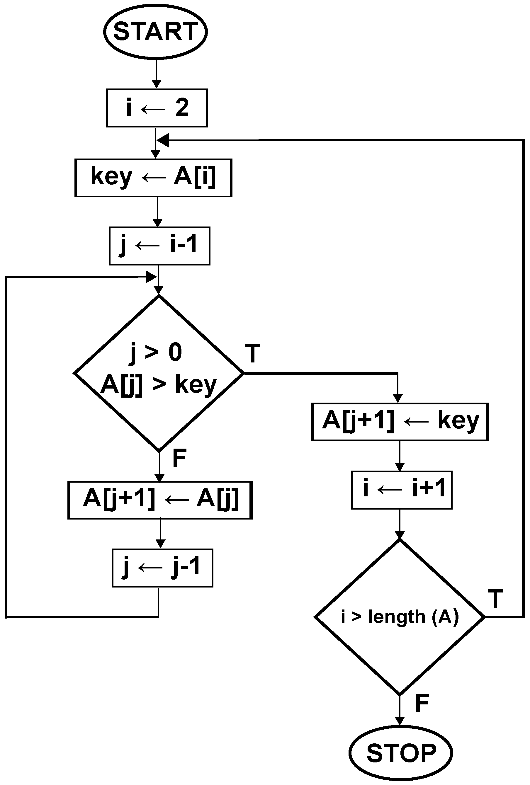
In this section, the considerations presented so far will be applied to sorting; as an example, insertion sort is presented. This is a quite simple procedure of sorting that is established on the observation of a bridge player who sorts his or her cards. He or she takes cards one-by-one from the heap and starts searching for the right position from left to the right. This structure is described by algorithm pseudocode and a flowchart.
1   for j ← 2 to length(A) do
2      key ← A[j]
3      i ← j-1
4      while (i > 0 and A[i] > key) do
5         A[i+1] ← A[i]
6         i ← i-1
7      A[i+1] ← key
It is very easy to see that this algorithm consists of two loops (
Figure 1). The external one is used to sort all data from the input set; the internal one finds the right place in the output set for successive sorted keys to form the input set. The calculations’ computational complexity is based on the number of internal loop executions (or equivalently, on the number of executions of the fourth line of code above), and this loop is crucial for our considerations. Let us note that if we focus on our algorithm as a net of connections in which sorted keys flow through existing paths, conditions checked in the fourth line of the pseudocode decide how long sorted data will stay in the internal loop. If we compare this loop to the trap for input data, it is easy to see that the amount of time for which the trap is active depends on three conditions: two of them are expressed explicitly; the third one is a matter of algorithm feedback. The first condition
i > 0 expresses the actual position in the input set; index
i is proportional to the size of input, so the loop will be longer as
i grows. The second condition depends on the values of the sorted keys; if the value of sorted key from the input set is small, the trap lasts longer than in the case when the sorted keys have large values. The third condition is very visible if we focus on algorithm behavior in terms of the interaction between the algorithm and the data structure, because the duration of the internal loop is also related to the number and values of keys sorted so far and is expressed by condition
A[i] > key (note that as the algorithm works, each sorted key is put into the first part of table
A[i]). The existence of feedback in this algorithm leads to the following cases: if in the condition in the fourth line of the pseudocode (
i > 0 and A[i] > key), only the first part
i >
0 is met, the feedback is simple, and as a result, the underlying process is short term. This is caused by the fact that the internal loop stops if the sorted key has the minimal value, whereas the condition
A[i] >
key is a part of the feedback with a possible memory effect that implies the existence of long-term processes; internal loop executions (trap) end depending on the input and output sets’ properties.
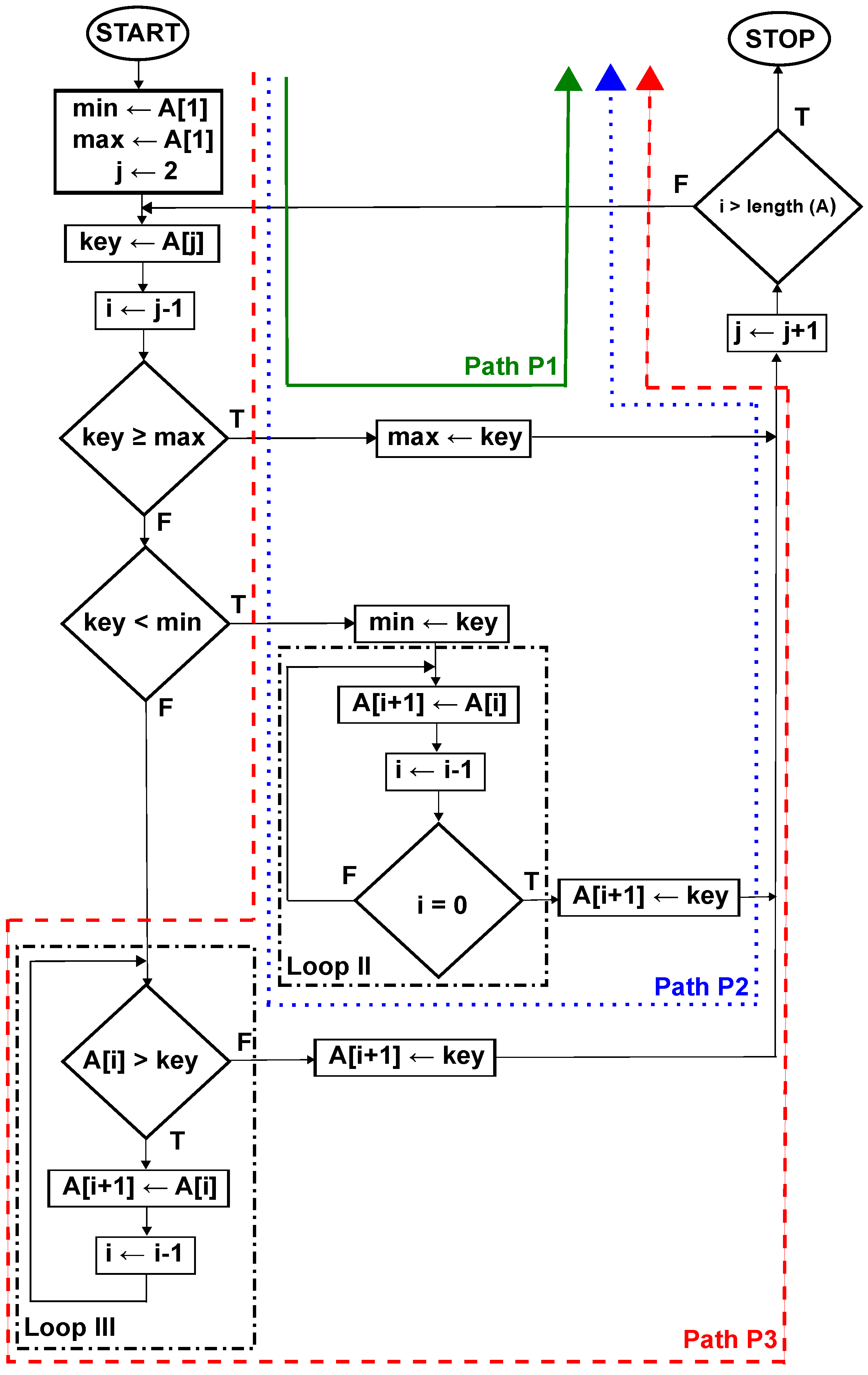
These considerations can be presented on a special flowchart (
Figure 2) that is an extended version of the diagram presented in
Figure 1. This new diagram is a result of some small modifications in our algorithm. These modifications help us to show a possible dynamical behavior of insertion sort. In the modified diagram (
Figure 2), two new variables are introduced, namely:
min and
max. They hold information about the minimal and maximal values of the so far sorted keys. As was stated above, the condition that opens the internal loop in the analyzed algorithm consists of two logical sub-conditions. They are joined by logical operator
and; as a result, this loop is executed if they are both fulfilled. However, this important condition can be broken into three cases. The first one is devoted for checking
A[j] ≥
max and, as a result, can be used to choose the shortest of all possible paths in the algorithm. This case is responsible for sorting keys with the maximal value. This path is always taken in the optimistic case (
Figure 2, solid (green) line), and it is easy to note (assuming that each operation in the whole diagram flow takes exactly the same amount of time) that the total time
needed for flow through this path is
(where
c stands for the number of intermediate steps in path P1 denoted by the solid (green) line in
Figure 2, like
min ← A[1],
max ← A[1],
etc.), giving the classical computational complexity expressed by
.
The second condition checks if
A[j]<
min and is met when the sorted key is minimal so far. As a result, all keys sorted so far have to be moved to the right in the output. Similarly to the first condition, this is the pessimistic case if all sorted keys follow this path (dotted (blue) line in (
Figure 2). Because in this case, for each sorted key, there is the need to execute Loop II and the number of these loop executions is
, the total time
needed for flow through this path is
(where
c again denotes the number of intermediate steps, like
min ← A[1],
A[i+1]←
key,
etc., in path P2, denoted by the dotted (blue) line in
Figure 2). Because
, the classical computational complexity for this case is expressed by
.
However, there is a third possibility, when any of the above conditions are not met; thus, the third condition
A[i] > key is checked. It dictates how long the Loop III will last (
Figure 2, dashed (red) line, path P3). In contradiction to the second case, where the loop duration is dependent on the number of keys sorted so far (index
i), this time, the loop duration depends also on the values of keys sorted so far or, in other words, on algorithm output.
The determination of the behavior of the modified algorithm when the flow through all possible Px paths is needed can be given assuming that:
is a set of input data instances with size n;
d is one instance of input data;
is the needed number (or equivalently time) of path Px (including loops) executions for instance d with size n;
is a random variable with values for ;
is a probability distribution of (the probability that the algorithm will do k path Px (including loops) executions or equivalently for an input set with size n).
If the set
is finite, each input instance is equiprobable. If the probability distribution of
is known, the calculations of its average value are possible by:
leading to the average case computational complexity.
The set
consists of all possible
permutations (instances) of
n-element sets. If
, then
has two elements:
In the modified procedure, sorting of this instance requires, respectively: path P1 with one execution and P2 with two executions of Loop II; path P1 with two executions. For
, the details are in
Table 1.
For
, both cases can appear with
; thus, the average number of path executions according to Equation (
1) is equal:
. For
, we have
, and the average complexity equals:
.
Nothing can be said about the behavior of
having the information about two cases. Thus, for
,
Table 2 was made, where one can find:
for
,
for
.
Based on the information from
Table 2, it is seen that
is a linear function of
n, and it might be expected that
is given by
. Indeed,
is represented as:
and this function is
, showing us that in the average case, the modified algorithm has a computational complexity the same as in the pessimistic case.
The existence of this feedback has a strong influence on algorithm behavior because:
dynamical behavior of this algorithm is possible [
21];
the third path can be seen as a parasite path (loop); it appears as a consequence of interaction between the algorithm and the input set;
the first two cases can be described by a mathematical relation that exactly determines the loops’ duration (or equivalently, the number of necessary dominant operations) for each sorted key; in other words, this number is deterministic;
in the third case, a non-deterministic behavior can appear and, as a consequence, the dynamical changes in the number of necessary dominant operations leading to the long-term processes;
the flow in this algorithm can have a turbulent nature.
Let us focus on the possible deterministic and non-deterministic behavior of the analyzed algorithm. Usually, it is assumed that typical algorithms are deterministic because, for each step, they have very well-defined successive steps. However, if we follow our previous remarks and focus on the data flow inside the algorithm, the definition of deterministic behavior can look a little bit different: it will refer to the exact count of the number of dominant operations for each processed element. In the case of insertion sort, it is possible to express this number for the best and worst cases in a very simple way by equation; for the rest of the cases, it can be determined based on the analysis of inversions and runs [
18], but this is not so simple. Especially, it is quite easy to calculate the number of inversions (situations where input sets’ successive keys are in reverse order or unsorted), but there are still some unsolved problems in the case of runs (situations where input keys are in the right order). As a final result for the optimistic and pessimistic cases for each key from the input set, one can exactly indicate the number of executed dominant operations: respectively, this is one and
, where
i denotes the index of the sorted key from an input set of size
n. However, both cases are only two of
possible ones (called input instances), and for most of the rest, based on the classical approach, it is impossible to give this number by equation. If we refer once again to the concept of flow, it can be said that pessimistic and optimistic cases refer to the laminar flows, whereas the others represent the turbulent flows. Typically, if the best and worst cases of computational complexity for an algorithm vary, one can follow average computational complexity analysis, but this gives a description in terms of asymptotic notation (here, given by
). This complexity measure is based on the idea of averaging, and nothing interesting can be said about the exact behavior (flow control) of the algorithm expressed in the number of necessary dominant operations (see
Figure 3). In other words: if we refer to the concept of processing as a flow, we cannot use the traditional approach, because it will not allow us to see some interesting phenomena.
In our approach, we apply the concepts of statistical mechanics, but the description of the algorithm behavior will not be given in terms of averaging, but in terms of statistical analysis of the time series representing the computational costs of the processing (the number of dominant operations for each processed element from the input set).
4. Entropy Production
Different approaches in the description of sorting procedures in terms of entropy production are known in the literature. In [
22], it is shown how the entropy as the measure of the input data uncertainty can be related to the computational difficulty of the given problem instance. In [
23], the total computational cost of the algorithm was shown as a function of the entropy of the input (output) distribution. Following the remarks from
Section 2, we stated that sorting is related to the introduction of order into a processed set. If we refer to physics, this means that the energy necessary for processing, which is delivered to the computer performing the sorting procedure, is used to decrease the entropy in the input (unordered) set. During processing (
i.e., a flow of elements from the input set), entropy from the input set is carried outside. In this analysis, we refer to the behavior of a Turing machine; thus, it is assumed that the entropy flow is only caused by the ordering procedure. As was noted in
Section 3, the insertion-sort algorithm can have dynamical behavior due to the existence of feedback. In order to determine the levels of entropy production, we refer to [
24], where the following approach was proposed.
Let
n be the size of a processed set and
denote the position of successively processed elements from the input set,
. Both internal and external loops need to be executed in insertion sort (given in
Figure 1) to process the input set. The number of executions for each key is given by
M, and its maximal value is
when the pessimistic case is sorted, while the minimal value is
when the optimistic case is processed. For each key, by
, we denote the number of external loop executions, and it is always equal to one; by
, we denote the number of all necessary internal loop executions, and it can change from zero (optimistic case) to
in the pessimistic case. By
, we denote the number of those internal loop calls that are not executed because of input set properties. Obviously, it is clear that
.
The amount of entropy that is removed during processing for each sorted key can be calculated based on the number of
W possible configurations (microstates) of the number of both loops’ executions. This quantity is given as the number of all possible combinations
multiplied by
[
24]; thus:
This result is consistent with the idea of permutations of a multiset (see, for example, Donald, E. Knuth survey in [
18] and the references therein).
In the optimistic case, for each key,
equals:
In the pessimistic case,
equals:
The obtained results can be a little surprising, but in the pessimistic case, the inverse order in the input set is still a kind of order; thus, the amount of entropy carried outside is on the lowest possible levels in both cases. Taking into account the Onsager relations [
25,
26], our system (processing machine) is in a (quasi)equilibrium state, where the entropy production is minimal. As confirmation, let us consider the number of microstates
W in other cases. If at least one excess dominant operation for key
is needed,
i.e.,
,
,
, we have:
and the number
W is greater than in the
or
cases.
The maximum entropy production occurs when
,
i.e., when the number of internal loop executions equals half of all possible executions (
). For some values of
, this value can be found in
Table 3, where the entropy
for each sorted key is also calculated using the Boltzmann–Gibbs formula,
with
.
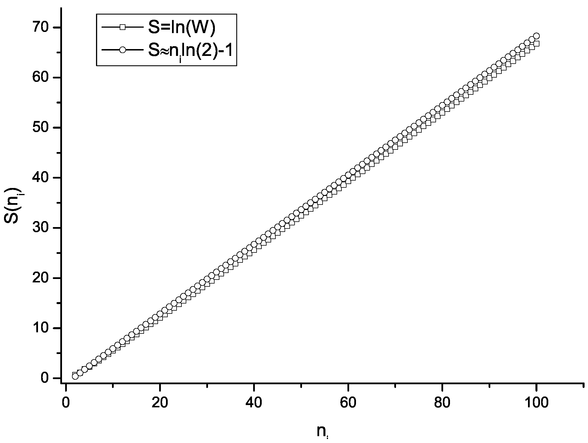
Plotting
versus (
Figure 4) illustrates that in the average case (
i.e.,
), the entropy growth tends to be linear for
.
This can be confirmed if one notes that when
, the number of possible loop configurations
W for the even number of keys
can be obtained as
for odd number of keys
, it is given as:
Thus, the entropy
can be calculated as:
Equation (
7), for
, can be written as:
The approximation of the entropy production given by Equation (
7) shows (
Figure 4) that for the average case, the level of (extensive) entropy production for each key
i is approximately represented by the linear function
. It should be noted that this is again consistent with Onsager reciprocal relations [
25,
26] and indicates that in the system, a thermodynamic non-equilibrium state exists, with maximum, but linear entropy production.
It is also possible to show some calculations for other cases. Equation (
6) shows that when at least one excess dominant operation is done, the number of microstates is greater than in optimistic and pessimistic cases. This equation allows one to establish formulas for exact calculations of the number of microstates. This is possible if we use the following reasoning: if one excess dominant operation is done, we have:
For two dominant operations, this is:
If we denote the number of necessary dominant operations by
(for the
i-th key from the input set), the number of microstates
W can be expressed as:
If
, the approximate calculations of
W are almost impossible on typical computers. However, taking into account that we are interested in calculations of entropy assuming that for each key, it is given by
, Equation (
10) can be rewritten as:
Because
, finally, we have:
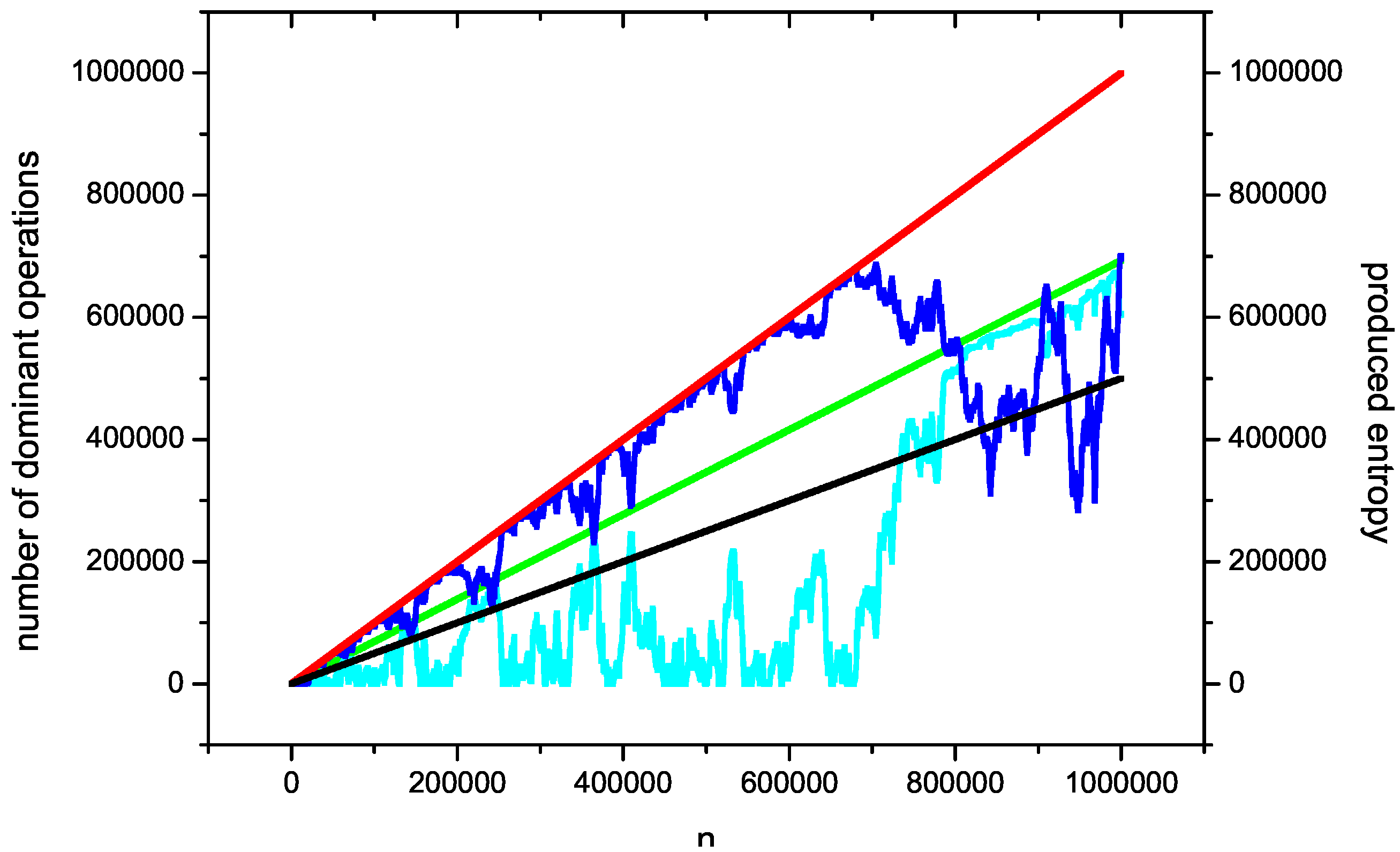
Figure 5 shows one example of a sorting process with the trajectory of entropy production during processing. The sorted set has
elements. Here, we assume that for each key
, the produced entropy
is extensive. For the average case, it grows linear, thus the total amount of produced entropy during sorting such a case by insertion sort can be expressed as
, which indicates the direct relationship between the problem of entropy production and the average case of the computational complexity of the insertion-sort algorithm. It is a very interesting problem itself, because the questions arise: Do such references exist for different sorting algorithms, and is it possible to use the concepts of other entropies (for example, nonextensive ones [
27]) in such calculations?
5. Influence of the Input Set on Dynamical Behavior
Equation (
3) shows the number of possible microstates for each successive sorted key. Usually, it is assumed that such a set is a collection of elements that is processed by a Turing machine. From the mathematical point of view, this collection is one of the possible permutations
of the
n-element set [
18], and this is a typical approach in combinatorics. One can assume that each sorted element is independent of the others, but in our considerations, we focus on the situation where there can be, but does not have to be, some level of correlation. Let us note that the input set can have
possible arrangements of key values. In many of them, one can indicate the existence of parts with many inversions or long runs. This situation is usually analyzed by a mathematical approach based on combinatorics with some existing open questions [
18]. We propose a different approach, because we treat computer processing in terms of a flow. This approach continues the considerations presented in
Section 3.
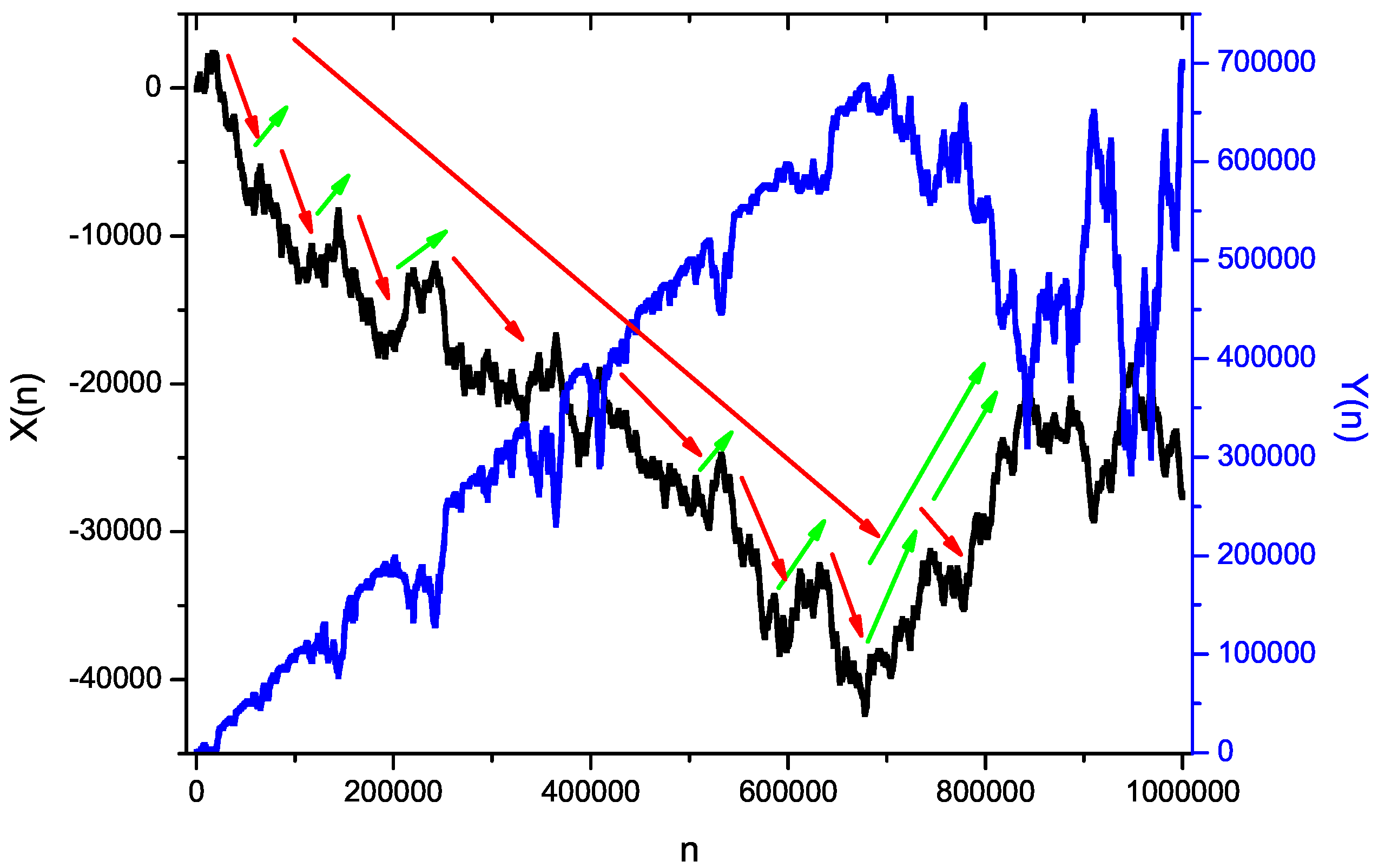
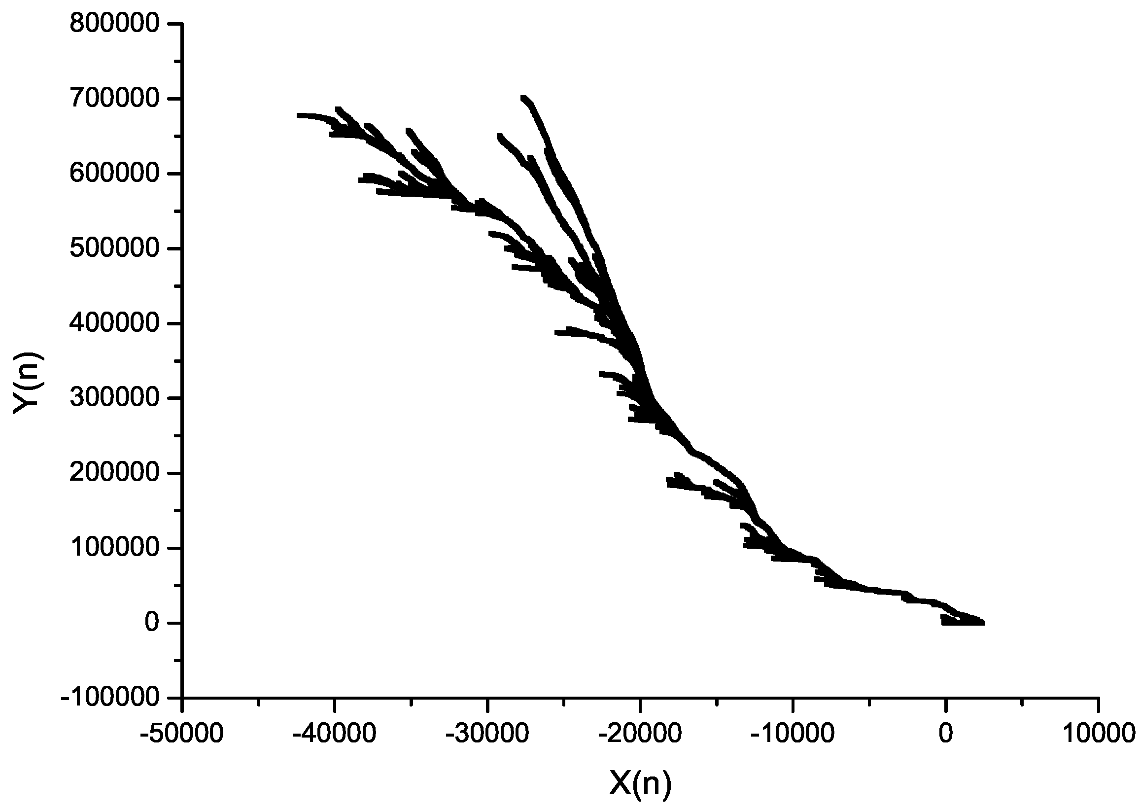
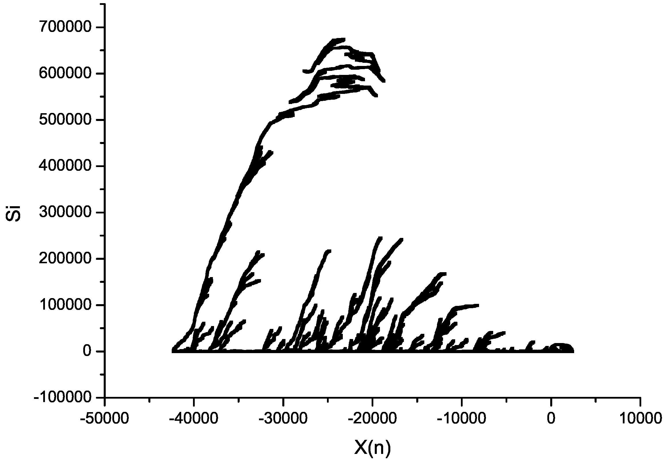
Below, we assume that the input set is a time series. For example, it can be generated as a trajectory of some process; here, it is proposed to use the concept of fractional Brownian motion (fBm), because this process has many features that are very useful in our considerations. The most important is the fact that its statistical self-similarity (described by Hurst
H parameter) can be used for the description of the statistical properties of the dependencies between the values of keys and, thus, the existence of inversions and long runs. It is known that the trajectories of fBm for values of
have long trends (property of persistence) that, for our sorting procedure, can be understood as local pessimistic and optimistic cases (see
Figure 6). The property of graphical self-similarity (to be more precise, self-affinity) shows that in each such trend, there are other minor trends.
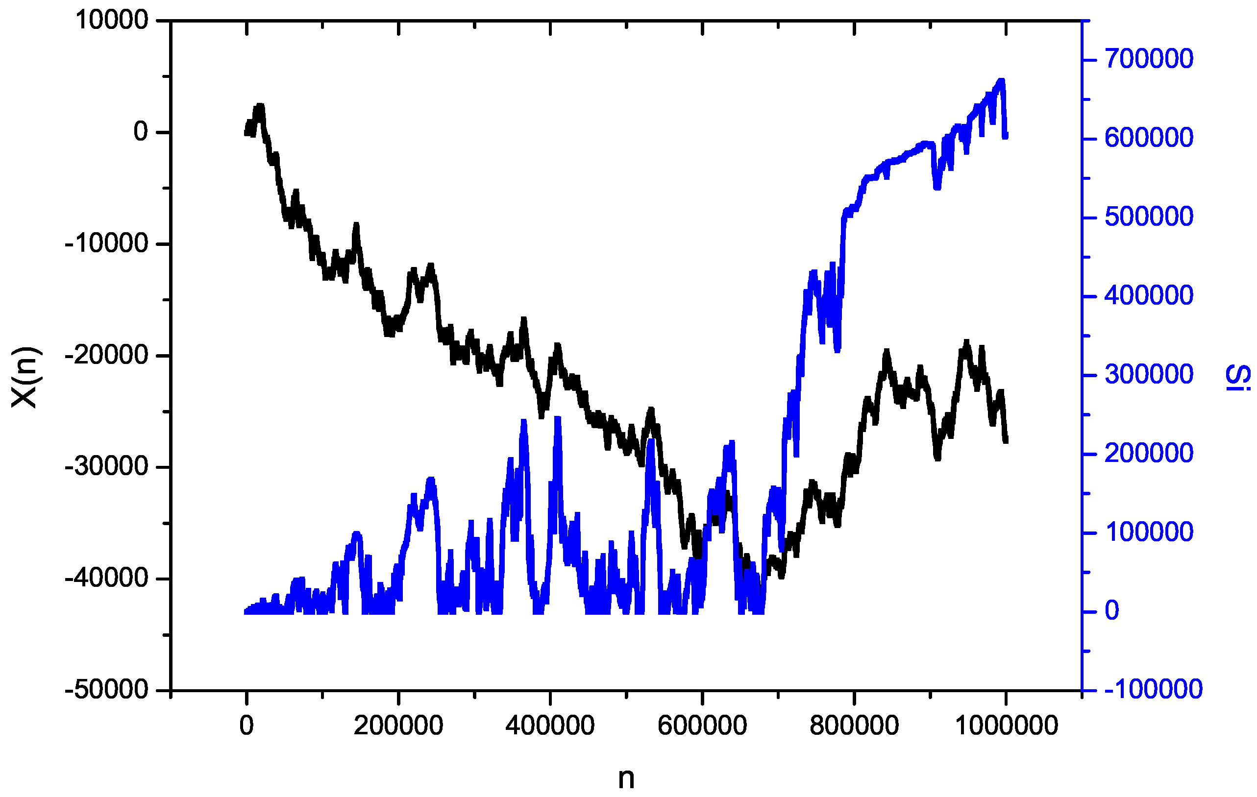
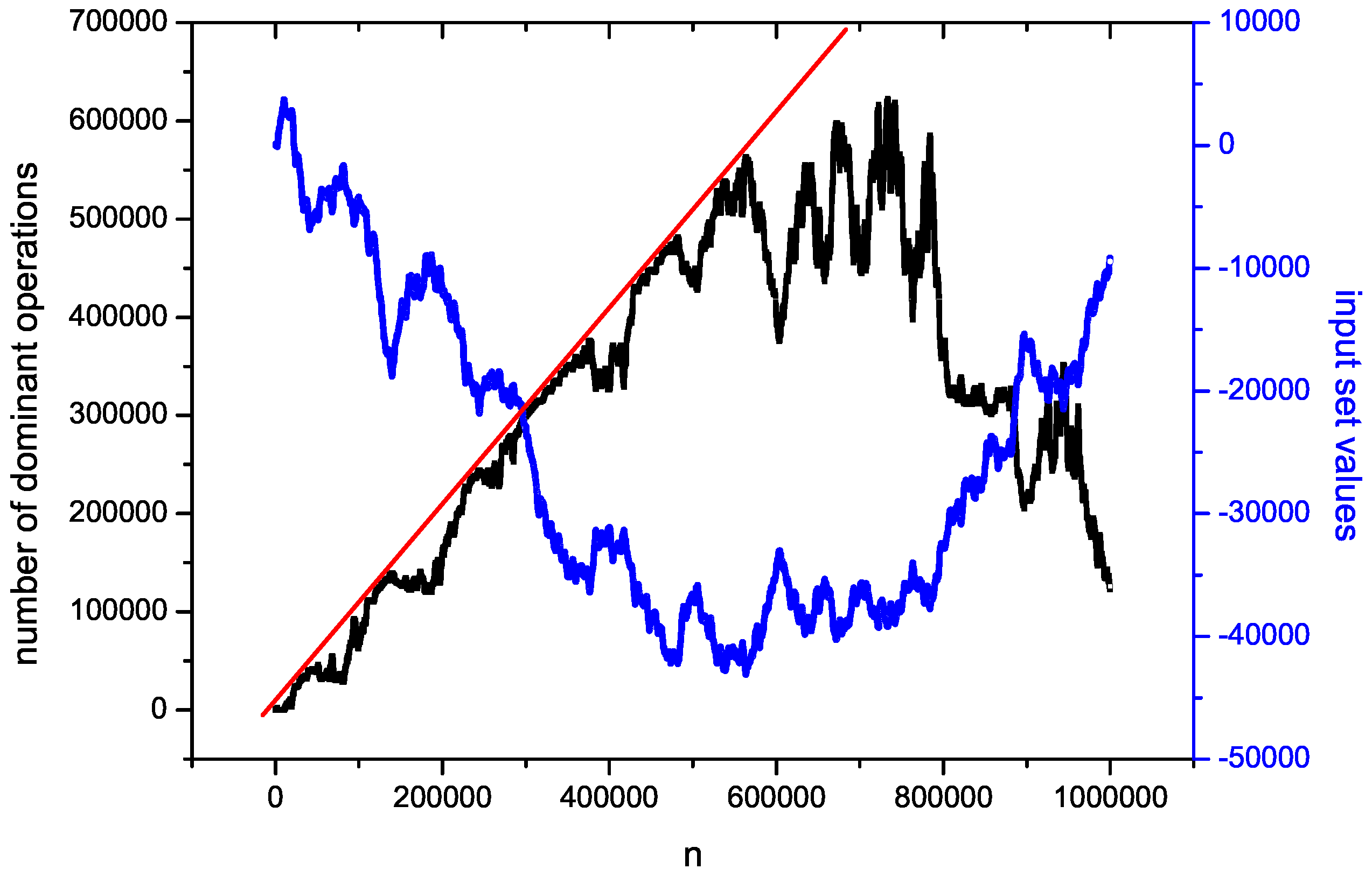
Recorded quantities of dominant operations for the insertion-sort procedure show not only the behavior of our algorithm (
Figure 6), but also how produced entropy
behaves during sorting according to Equation (
12). One example is shown in
Figure 7: the sorted set is a trajectory of fBm with
. The amount of produced entropy is not only dependent on visible trends, but on the situation when the trend is changing from falling to rising and reverse.
As noted in
Section 3, a feedback exists in this algorithm, and it has a strong influence on the procedure behavior. In order to show this influence, the plot in
Figure 8 was created, illustrating the relations between values of input keys
and the number of dominant operations
, and the plot in
Figure 9 illustrates the relations between the values of input keys
and produced entropy
.
As can be seen
Figure 6,
Figure 7,
Figure 8 and
Figure 9, behavior of the analyzed algorithm is very complex. Let us note the feedback existing in the algorithm; its existence influences the number of necessary dominant operations for each sorted key. If successive keys from the input are ordered according to relation <(rising trend, optimistic case) or respectively according to relation > (falling trend, pessimistic case), the number of dominant operations for each sorted key will be equal to one or
, respectively, and such a complex behavior in both cases will not be visible. Now, let us also note that our sorting procedure is done by a physical machine (computer) that is used not only to perform this process, but also, it is expected that it controls its possible dynamical behavior. It is clear that understanding the idea of processing is more complicated than it seems to be: it is not only a simple mathematical operation (transformation of bits), but also a process that can be very complex.


