Article

Tea Category Identification Using a Novel Fractional Fourier Entropy and Jaya Algorithm

1
School of Computer Science and Technology, Nanjing Normal University, Nanjing 210023, China
2
Jiangsu Key Laboratory of 3D Printing Equipment and Manufacturing, Nanjing 210042, China
3
Guangxi Key Laboratory of Manufacturing System & Advanced Manufacturing Technology, College of Mechanical Engineering, Guangxi University, Nanning 530021, China
4
Department of Mathematics and Mechanics, China University of Mining and Technology, Xuzhou 221008, China
5
Engineering School (DEIM), University of Tuscia, Viterbo 01100, Italy
6
Department of Mechanical Engineering, Sardar Vallabhbhai National Institute of Technology, Surat 395007, India
7
School of Natural Sciences and Mathematics, Shepherd University, Shepherdstown, WV 25443, USA
*
Authors to whom correspondence should be addressed.
These authors contributed equally to this work.
Entropy 2016, 18(3), 77; https://doi.org/10.3390/e18030077
Submission received: 14 October 2015 / Revised: 15 January 2016 / Accepted: 16 February 2016 / Published: 27 February 2016
(This article belongs to the Special Issue Computational Complexity)

Abstract

:
This work proposes a tea-category identification (TCI) system, which can automatically determine tea category from images captured by a 3 charge-coupled device (CCD) digital camera. Three-hundred tea images were acquired as the dataset. Apart from the 64 traditional color histogram features that were extracted, we also introduced a relatively new feature as fractional Fourier entropy (FRFE) and extracted 25 FRFE features from each tea image. Furthermore, the kernel principal component analysis (KPCA) was harnessed to reduce 64 + 25 = 89 features. The four reduced features were fed into a feedforward neural network (FNN). Its optimal weights were obtained by Jaya algorithm. The 10 × 10-fold stratified cross-validation (SCV) showed that our TCI system obtains an overall average sensitivity rate of 97.9%, which was higher than seven existing approaches. In addition, we used only four features less than or equal to state-of-the-art approaches. Our proposed system is efficient in terms of tea-category identification.

1. Introduction

Tea is a beverage prepared by pouring boiled water over its leaves [1]. As a medicinal drink, there is now increasing evidence that antioxidants contained in tea could help resist diseases, such as breast cancer [2], neurodegenerative disease [3], skin cancer [4], Parkinson’s disease [5], prostate tumor [6], Alzheimer’s disease [7], cardiovascular disease [8], colon cancer [9], etc.
The tea-category identification (TCI) is of importance for controlling fermentation time so as to obtain the expected tea. Six main types of tea were produced, including: white tea, yellow tea, green tea, Oolong tea, black tea, and post-fermented tea. In China, green, black, and Oolong tea are the most popular categories [10]. Table 1 lists their characteristics.
In the past decade, there are two novel types of methods, viz., hardware and software, for tea classification. The former is aimed at devising new devices while the latter is aimed at designing new algorithms based on computer vision, which has proven to be better than human vision in many fields [11,12,13].
Some researchers proposed the use of new measurement devices. Zhao et al. [14] employed near-infrared (NIR) to identify three categories of tea. The identification accuracies were all above 90%. Chen et al. [15] employed NIR reflectance spectroscopy to classify three different teas. Herrador and Gonzalez [16] chose eight metals as chemical descriptors, with the aim of differentiating three categories of tea. Later, Chen et al. [17] designed an electronic nose based on odor imaging sensor arrays for identify fermentation degrees. Szymczycha-Madeja et al. [18] developed a method by flame atomic absorption spectrometry (FAAS) and inductively coupled plasma optical emission spectrometry (ICP OES) to determine (non-)essential elements in black and green teas. Liu et al. [19] utilized the electronic tongue to process 43 pieces of data of black and green tea. Dai et al. [20] employed E-nose for quality classification of Xihu-Longjing tea. The aforementioned methods yielded excellent classification results; nevertheless, they needed expensive sensor devices and suffered from lengthy procedures.
In the last decade, computer vision based approaches were introduced to help develop TCI systems. However, computer vision systems are composed of intervolved parts that interact dynamically at different scales in space. In addition, the complexity in the TCI system gives rise to large-scale dynamics that cannot be summarized by a single rule. The issues in modeling TCI systems require the development of novel computational tools. For instance, Chen et al. [21] employed 12 color features and 12 texture features. Then, they employed principal component analysis (PCA) and linear discriminant analysis (LDA) to generate the classification system. Jian et al. [22] classified and graded the tea on the basis of color and shape parameters. Genetic neural-network (GNN) was used to build the identification system, which yielded promising effects of identification with eight parameters of color and shape. Laddi et al. [23] suggested acquiring tea granule images using a 3-CCD camera in the illumination condition of dual ring light. Gill et al. [24] overviewed various computer vision based algorithms for texture and color analysis with a special orientation towards monitoring and grading of made tea. Zhang et al. [25] combined three different types of features (shape, color, and texture) to identify fruit images. Tang et al. [26] extracted features from green tea leaves by combining local binary pattern (LBP) and gray level co-occurrence matrix (GLCM). Akar and Gungor [27] integrated multiple texture methods and normalized difference vegetation index (NDVI) to the random forest algorithm, in order to detect tea and hazelnut plantation areas. Wang et al. [28] utilized wavelet packet entropy (WPE). They then combined fuzzy technique with support vector machine (SVM), and named it fuzzy SVM (FSVM). Their method yielded a promising result of 97.77% recall rate. Those methods used simple digital cameras rather than expensive devices, but the identification performances did not meet the requirement of practical use.
In this study, we proposed a novel approach on the basis of computer vision and machine learning, with the aim of improving the classification sensitivities of each category. To improve the accuracy of TCI, we introduced a relatively new feature descriptor—fractional Fourier entropy (FRFE) [29]—that combines two successful components: fractional Fourier transform (FRFT) and Shannon entropy (SE). We also introduced the Jaya algorithm to train the classifier. Jaya was proposed by Rao [30]. There is no need to tune its algorithm-specific parameters (ASPs).
The structure of the rest of this paper is organized as follows. Section 2 describes the sample preparation. Section 3 and Section 4 show the feature extraction and reduction, respectively. Section 5 presents the classification method. Section 6 provides the experiments, results, and discussions. Finally, Section 7 concludes this study and provides the future research directions. The acronyms are explained in the Abbreviations section.

2. Materials

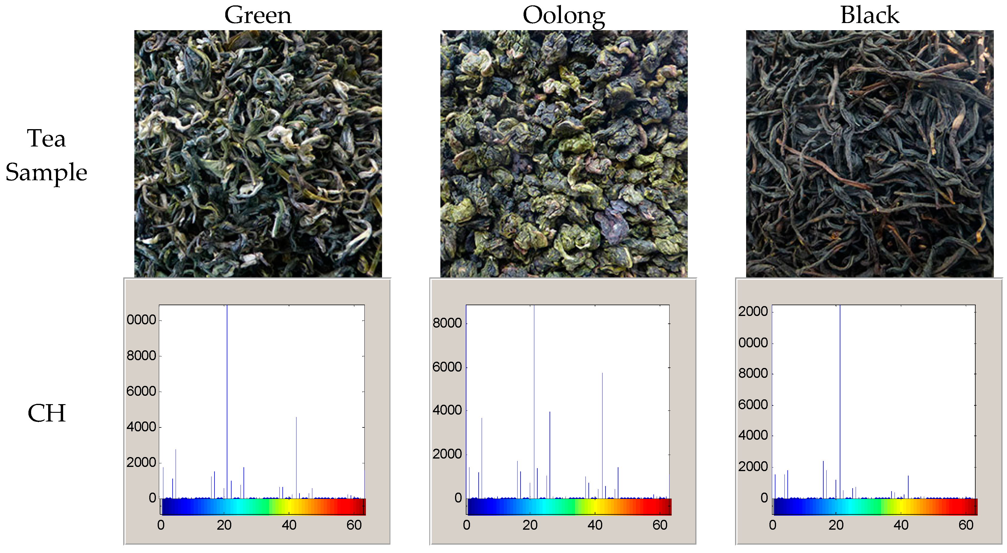
2.1. Tea Sample Preparation

Three-hundred samples of three categories of tea (green, black, and Oolong) were prepared. The tea samples originated from different areas in China. In order to augment the generalization capability of our TCI system, each category contained different brands.
Table 2 shows the sample settings. The green tea has 100 samples, originating from Guizhou, Henan, Anhui, Jiangxi, Jiangsu, and Zhejiang provinces. The black tea has 100 samples, originating from Yunnan, Fujian, Hunan, and Hubei provinces. The Oolong tea has 100 samples, originating from Guangdong and Fujian provinces.

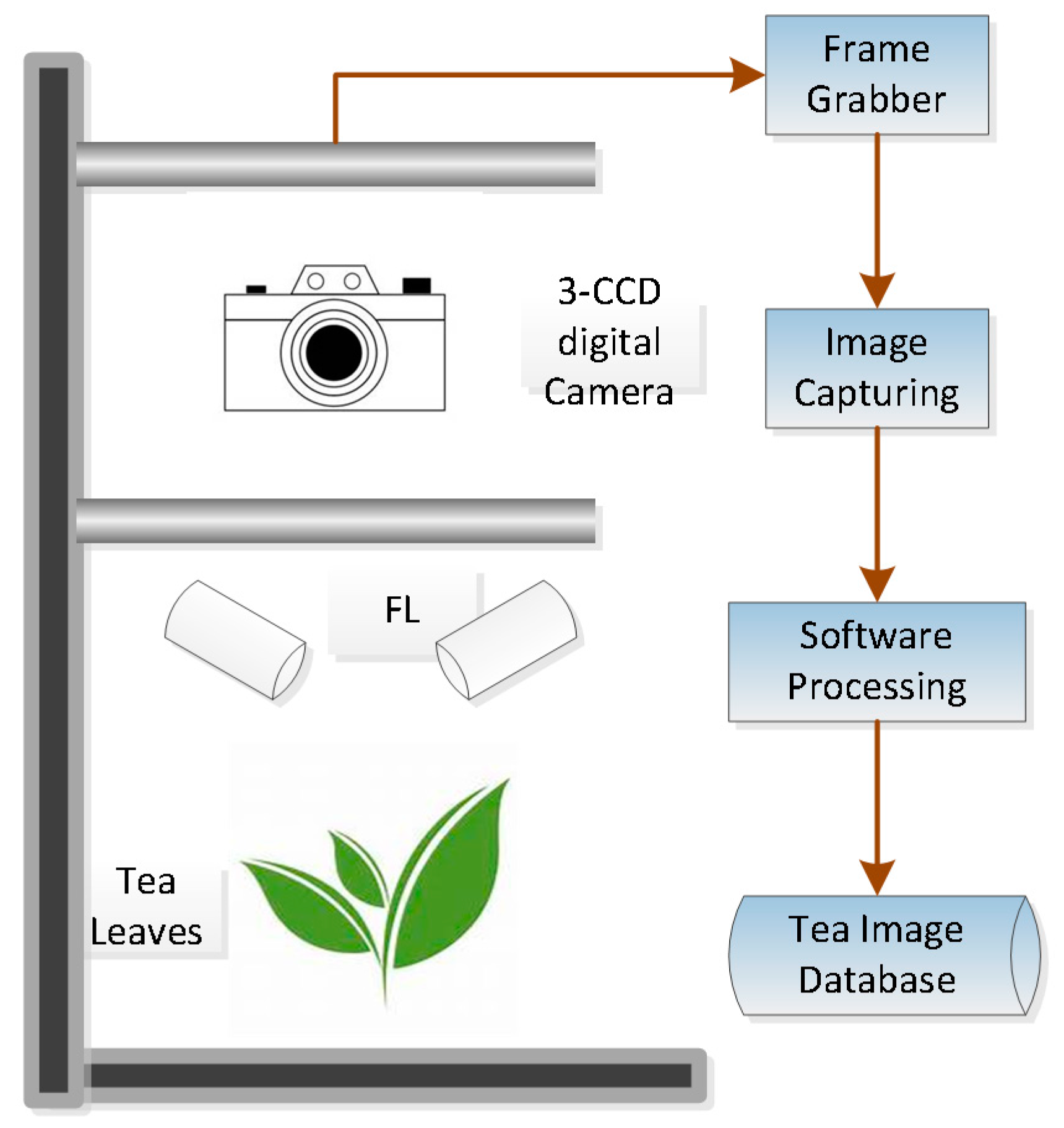
2.2. Image Acquiring

Figure 1 shows the TCI system used in this study. It consisted of five parts: (1) illumination system; (2) a camera; (3) a capture board; (4) computer hardware; and (5) computer software.
We spread the tea-leaves thinly over the tray, and then employed a 3-CCD digital camera to acquire tea images. Compared to 1-CCD cameras, 3-CCD cameras provide high-resolution images with lower noise [23]. The lighting arrangements were classified as two types: front or back lighting [31]. Front lighting (FL) is used to produce surface extraction, whereas the back lighting (BL) is used when production of a silhouette image is needed [24]. We used front lighting (FL) in this study.
The captured images are a size of 256 × 256 with 180 dpi. They are stored without loss in TIFF format. We used two-dimensional median filters to remove noise. The tea-leaves are not reused among the images. With the aim of using fresh tea samples, they were obtained when in stock within a four-month period.

3. Feature Extraction

3.1. Color Histogram

Diniz et al. [32] used a color histogram (CH) with the software ImageJ 1.44p as an analytical information to screen teas. Yu et al. [33] combined CH and texture information to classify green teas. CH represents the distribution of colors in a particular image [34]. CH counts the number of pixels that are of the similar color range. The procedure of CH contains two steps. First, we discretized each color channel (RGB) into four bins. Second, the whole image in RGB space was segmented into 4 × 4 × 4 = 64 bins. Third, we counted pixel numbers in each bin. The advantage of CH is its relative translation invariance and rotation invariance.

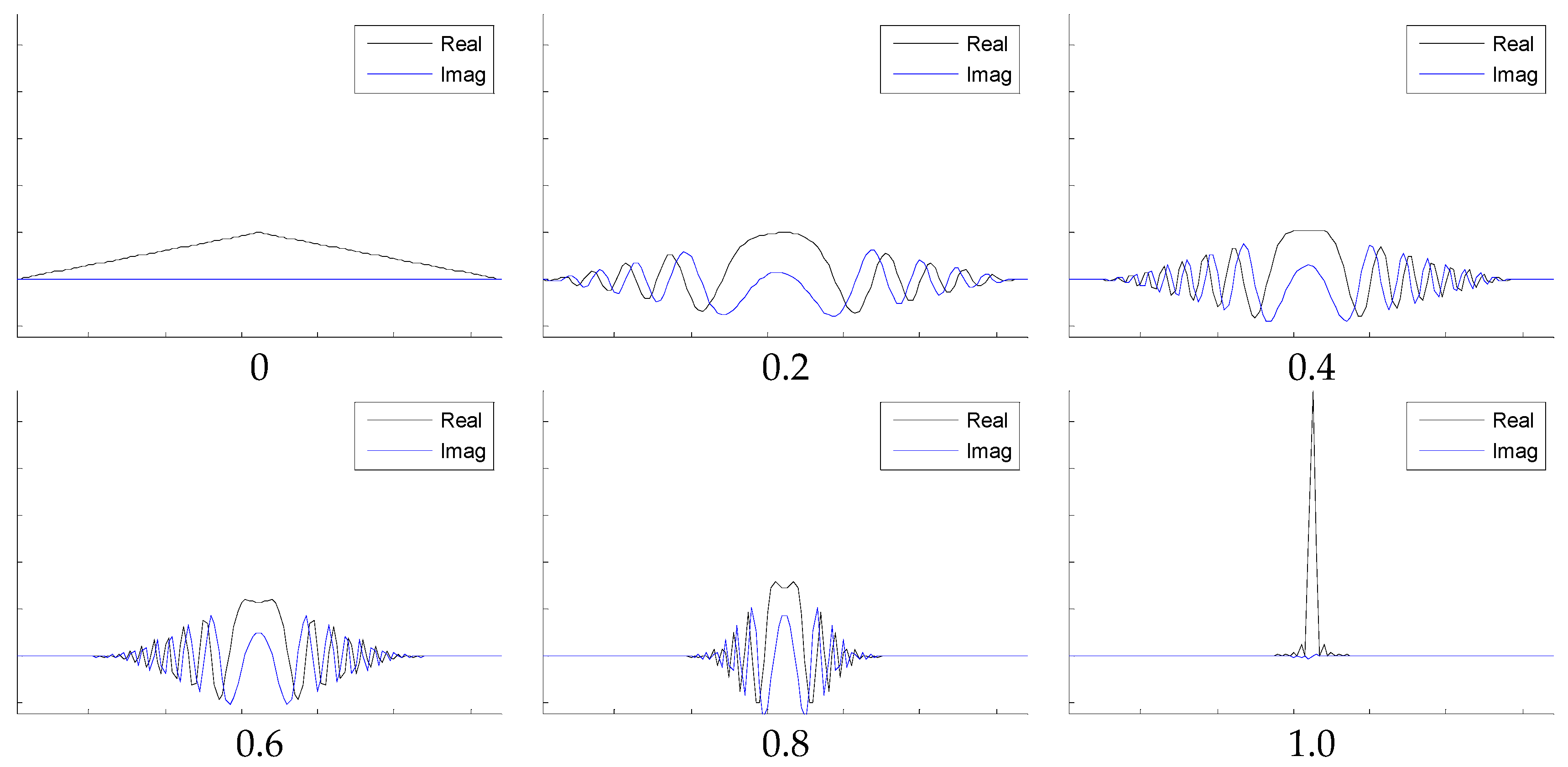
3.2. Fractional Fourier Transform

The α-angle fractional Fourier transform (FRFT) [35,36] of a particular function x(t) was denoted by Yα with following form:
Y α ( u ) = T α ( t , u ) x ( t ) d t .
Here, u denotes the frequency, t the time, and T the transform kernel is defined as
T α ( t , u ) = 1 j cot α × exp ( j π ( u 2 cot α 2 u t csc α + t 2 cot α ) ) .
Here, j represents the imaginary unit. For the tea images, we need to extend FRFT to the two-dimensional space. Two angles exist for 2D-FRFT, α and β [37,38,39,40]. Furthermore, the results of FRFT with angles from 0 to 1 are listed in Figure 2. A triangular signal tri(t) is used, and its frequency spectrum is sinc2(u) [41]. In the figure, black lines represent real components, and blue lines imaginary components.

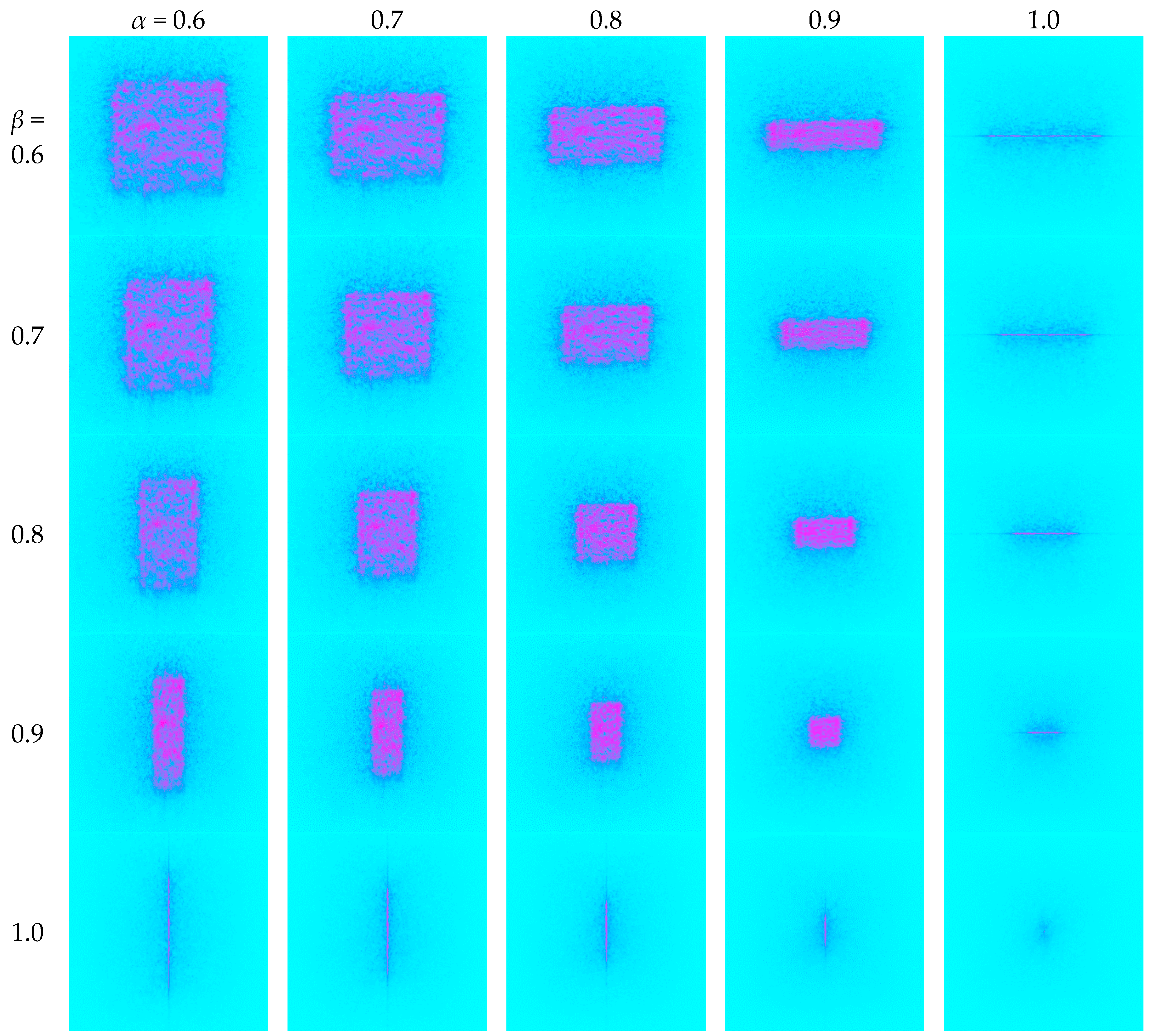
3.3. Fractional Fourier Entropy

We introduced a relatively new image feature of Fractional Fourier Entropy (FRFE), denoted by symbol E. Mathematically, we implemented Shannon entropy operator S on the spectrums obtained by FRFT Y:
E = S Y .
When FRFT was implemented over the tea leave images, 25 unified time-frequency spectrums were generated with various combinations of α and β. Suppose I represents a tea image, the FRFE can be written in a matrix as
E ( I ) = S [ Y ( I ) ] = S [ Y 0.6 , 0.6 Y 0.6 , 0.7 Y 0.6 , 0.8 Y 0.6 , 0.9 Y 0.6 , 1 Y 0.7 , 0.6 Y 0.7 , 0.7 Y 0.7 , 0.8 Y 0.7 , 0.9 Y 0.7 , 1 Y 0.8 , 0.6 Y 0.8 , 0.7 Y 0.8 , 0.8 Y 0.8 , 0.9 Y 0.8 , 1 Y 0.9 , 0.6 Y 0.9 , 0.7 Y 0.9 , 0.8 Y 0.9 , 0.9 Y 0.9 , 1 Y 1 , 0.6 Y 1 , 0.7 Y 1 , 0.8 Y 1 , 0.9 Y 1 , 1 ] ( I ) .
Here, Yα,β denotes an FRFT perform with α-angle along x-axis and β-angle along y-axis. We set both angles to vary from 0.6 to 1 with an equal increase of 0.1, because angles close to 0 will degrade FRFT to an identity operation.

4. Feature Reduction

4.1. Principal Component Analysis

Principal component analysis (PCA) reduces the dimension of a data set that is composed of a large number of variables, while it reserves the most significant principal components (PC). The common method to calculate PCA is based on the covariance matrix. Suppose a dataset X with dimensions of p and a size of N. We need to preprocess the dataset to have zero mean. First, the empirical mean of each feature was obtained by
u j = 1 N i = 1 N X ( i , j ) .
Afterwards, the deviation is yielded by mean subtraction
B = X e u T .
Here, B stores the centered data and e means an N × 1 vector of all 1s. The p × p covariance matrix C is generated
C = 1 N 1 B * B ,
where * denotes for the conjugate transpose symbol. The covariance matrix can give an eigendecomposition expression as
V 1 C V = D .
Here, D is a diagonal matrix fulfilled with eigenvalues (C). V is the matrix of eigenvectors. We rearrange the eigenvector matrix V and eigenvalue matrix D so that the eigenvalue is in a decreasing order. Remember that eigenvalue represents the distribution of variances from the source data among each eigenvector, we then select a subset of eigenvectors used for basis vectors. This is done by computing the cumulative variance for each eigenvector in the form of
G ( n ) = i = 1 n D ( i , i ) .
Finally, we select L principal components (PCs) that can cover variance that is above a threshold T of original variances,
G ( L ) G ( p ) T .

4.2. Kernel Principal Component Analysis

PCA can only extract linear structure information. Nevertheless, it cannot handle the dataset containing nonlinear structure. Kernel PCA (KPCA) is an extension of standard PCA. It transforms the input dataset into a higher dimensional space where PCA is then implemented. Note that the higher dimensional feature space is not required to be computed explicitly, because KPCA is simply implemented by computing the inner product of two vectors with a kernel function.
Several kernels are commonly used. The most commonly used is Gaussian Radial basis function (RBF) kernel with the form of
k RBF ( x , y ) = exp ( x y 2 2 σ 2 ) ,
where σ represents the scaling factor. Polynomial kernels are listed below
k pol ( x , y ) = ( x × y + b ) d ,
where b and d are parameters, which can be tuned by grid searching approach. σ is searched in the range of [1, 100] with increment of 10. b is searched in the range of [0, 1] with increment of 0.1, and d is in the range of [1, 5] with increment of 1. We termed the above polynomial kernel and RBF kernel based PCAs as POL-KPCA and RBF-KPCA, respectively.

4.3. Implementation

Revisit the feature extraction and reduction procedures, we proposed a composite feature set, which is composed of 64 color histogram (CH) features and 25 FRFE features. Afterwards, PCA, POL-KPCA, RBF-KPCA were employed to reduce the number of total features. Here, the threshold is set to that remained PCs should cover at least 99.5% variances of original full features. Figure 3 illustrates the flowchart of our feature-processing technique.
As a result, 89 features were extracted from a particular tea image. We used three feature reduction approaches (PCA, POL-KPCA, RBF-KPCA) to further reduce them.

5. Classification

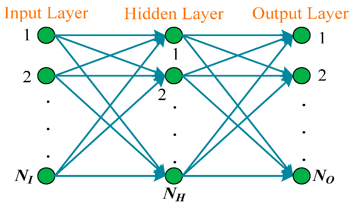
5.1. Feed-Forward Neural Network

There are many canonical classification techniques. In this paper, we employed the feedforward neural network (FNN), because it did not need information related to the probability distribution [42], nor the a priori probabilities of different classes [43].
Figure 4 illustrates the general one-hidden-layer (OHL) FNN. Within this model, there are three different types of layers: an input layer, a hidden layer, and an output layer. Their neuron numbers are represented as NI, NH, and NO, respectively. The activation function is selected as sigmoid and linear for the hidden layer and output layer, respectively.
To build the FNN to be equal to train the weights/biases of all neurons in the FNN, which is treated as an optimization problem, i.e., we need to obtain the optimal weights/biases in order to make minimal the mean-squared error (MSE) between real outputs and target outputs.

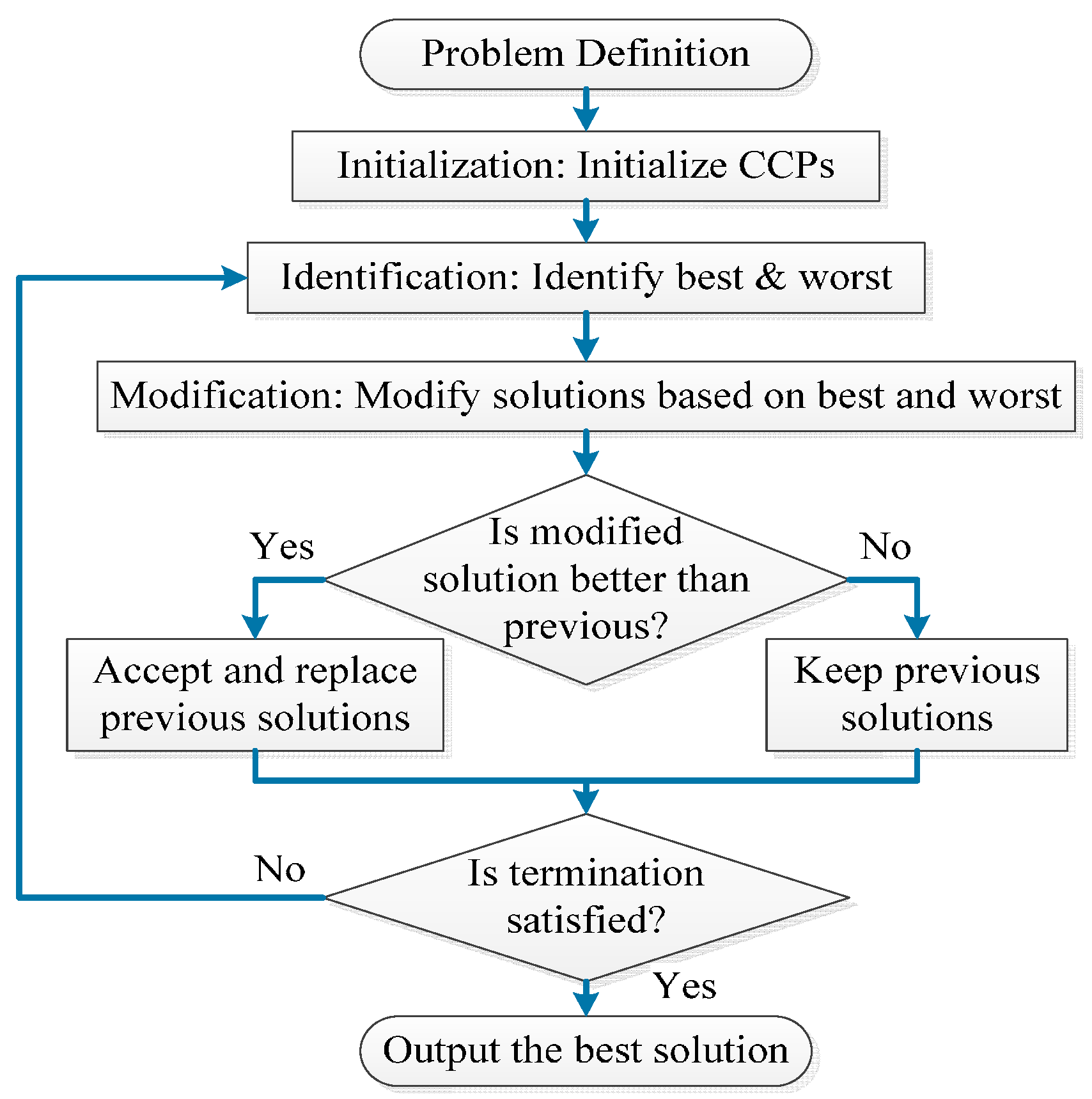
5.2. Optimization Methods

A variety of optimization methods exist for FNN training. Traditional methods include back-propagation (BP) [44], momentum BP (MBP) [45], and meta-heuristic algorithms: genetic algorithm (GA) [46], simulated annealing (SA) [47], artificial bee colony (ABC) [48], particle swarm optimization (PSO) [49], biogeography-based optimization (BBO), and fitness-scaled chaotic ABC (FSCABC).
The BP and MBP do not perform well on non-linear data [50,51]. For meta-heuristic approaches, they usually obtain better performances; however, they need to tune both common controlling parameters (CCPs) and algorithm-specific parameters (ASPs), which influence their performance and complicate their applications. Rao et al. [52] was the first to propose a meta-heuristic approach that does not require any ASP. They named their method as teaching-learning-based optimization (TLBO) [53]. Although TLBOs are widely used in various fields [54,55,56], it needs to be implemented at two phases (teacher phase and learner phase) [57].
Recently, a novel approach called Jaya (A Sanskrit word meaning victory) was proposed. Jaya not only inherits the ASP free of TLBO but is also simpler than TLBO. In addition, Rao [30] compared Jaya with the latest approaches, and they found Jaya ranks first for “best” and “mean” solutions for all 24 constrained benchmark problems and gives better performances over 30 unconstrained benchmark problems. In this study, we make a tentative proposal of using Jaya to train the weights/biases of feed-forward neural network (FNN), and we propose a novel classifier termed as Jaya-FNN.
Figure 5 shows the diagram of Jaya. Here, suppose b and w represent the index of best and worst candidates among the population, and suppose i, j, k is the index of iteration, variable, and candidate. Then A(i, j, k) means the j-th variable of k-th candidate in i-th iteration. The modification formula of each candidate can be written as
A ( i + 1 , j , k ) = A ( i , j , k ) + r ( i , j , 1 ) ( A ( i , j , b ) | A ( i , j , k ) | ) r ( i , j , 2 ) ( A ( i , j , w ) | A ( i , j , k ) | ) ,
where A(i, j, b) and A(i, j, w) represents the best and worst value of j-th variable in i-th iteration. The r(i, j, 1) and r(i, j, 2) are two random numbers in the range of [0, 1] generated at random. The second term “r(i, j, 1)(A(i, j, b) − |A(i, j, k)|” indicates the candidate should move closer to the best one, while the third term “−r(i, j, 2)(A(i, j, w) − |A(i, j, k)|” indicates that the candidate should move further away from the worst one (note the minus symbol before r). The A(i+1, j, k) is accepted if the modified candidate is better in terms of function values, otherwise the previous A(i, j, k) is maintained.

5.3. Statistical Setting

In this study, we used K-fold stratified cross validation (abbreviated as SCV) for statistical analysis. By K-fold SCV, the tea samples were partitioned into K mutually exclusively folds of approximately equal size and approximately similar class distribution. To give stricter results, the K-fold SCV was repeated 10 times. We assigned K as 10 for easy and fair comparison, since the recent literature all used 10-fold cross validation. In addition, the model was established each time the training set was re-generated.

6. Experiments, Results and Discussions

6.1. Color Histogram

Figure 6 shows one sample of three categories of teas. It also shows their corresponding color histogram (CH). The x-axis represents the 64 bins, while the y-axis represents the pixel number. Figure 6 validates the distribution of color histograms of green, Oolong and black teas were distinct from each other; therefore, the color histogram is an efficient measure for tea-category identification.

6.2. FRFT Results

Figure 7 shows the FRFT result of an Oolong tea image. As it shows, the FRFT degrades to standard FT when both α and β increase to one. The contents in FRFD suggest tea images contain a mass of information, so FRFT is a better tool that can provide more information than standard FT.

6.3. FRFE Results

Afterwards, we extract entropy information from each FRFD. The mean and standard deviation of each class is listed in Table 3. We can see that the FRFE is an extremely effective feature, such that the three tea categories can be segmented by the 25 FRFE features.

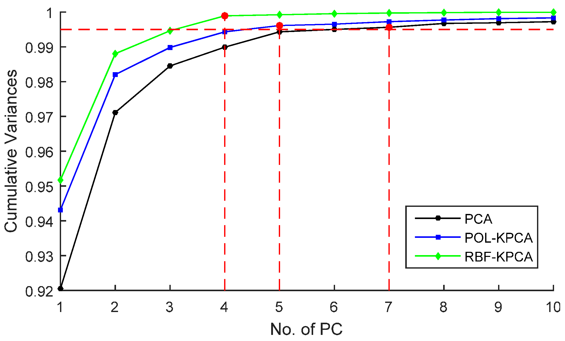
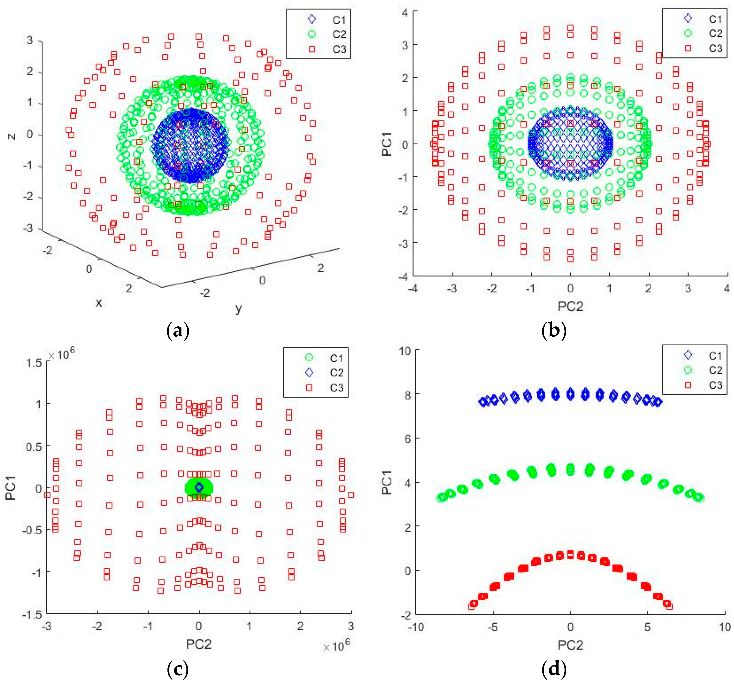
6.4. KPCA over Simulation Data

Figure 8 shows how KPCA extends the data to non-linear feature maps for simulation data. Figure 8a shows a three-dimensional three-class dataset. Points in class 1, class 2, and class 3 are distributed along three spheres with the same origin and different radii of 1, 2, and 3, respectively. Both PCA and KPCA reduced the features from 3 to 2. Figure 8b–d shows the feature reduction results by PCA, KPCA with polynomial kernel, and KPCA with RBF kernel, respectively.
We can find that the two PCs obtained by PCA cannot segment the data, since they are entangled with each other. The reduced features obtained by POL-KPCA do not overlap with each other, so they may be segmented in a nonlinear approach. Finally, the RBF-KPCA performs the best so its reduced data can be divided by linear methods. In addition, the RBF-KPCA can only preserve only one reduced feature (i.e., PC1), and it can still be easily classified. Although KPCA has the above advantage, it requires added complexity and additional model hyperparameters to tune.

6.5. KPCA over Tea Features

The 89 features of each tea image are reshaped as a row vector. Then, each 89-element feature vector of all tea images were justified to form one two-dimensional array. Figure 9 illustrates the curve of variance versus PC number by PCA, POL-KPCA, and RBF-KPCA approaches. The optimal parameters of the POL and RBF kernels were chosen by grid search technique with the aim of accumulating more variance with less number of PCs. They were implemented on the overall dataset.
From curves in Figure 9, we can see that the PCs selected under the same threshold of 99.5% are four, five, and seven for RBF-KPCA, POL-KPCA, and standard PCA, respectively. We can conclude that RBF-KPCA is superior to the other two approaches in reducing features in terms of cumulative variance. The result falls within the finding set out in Section 6.4.

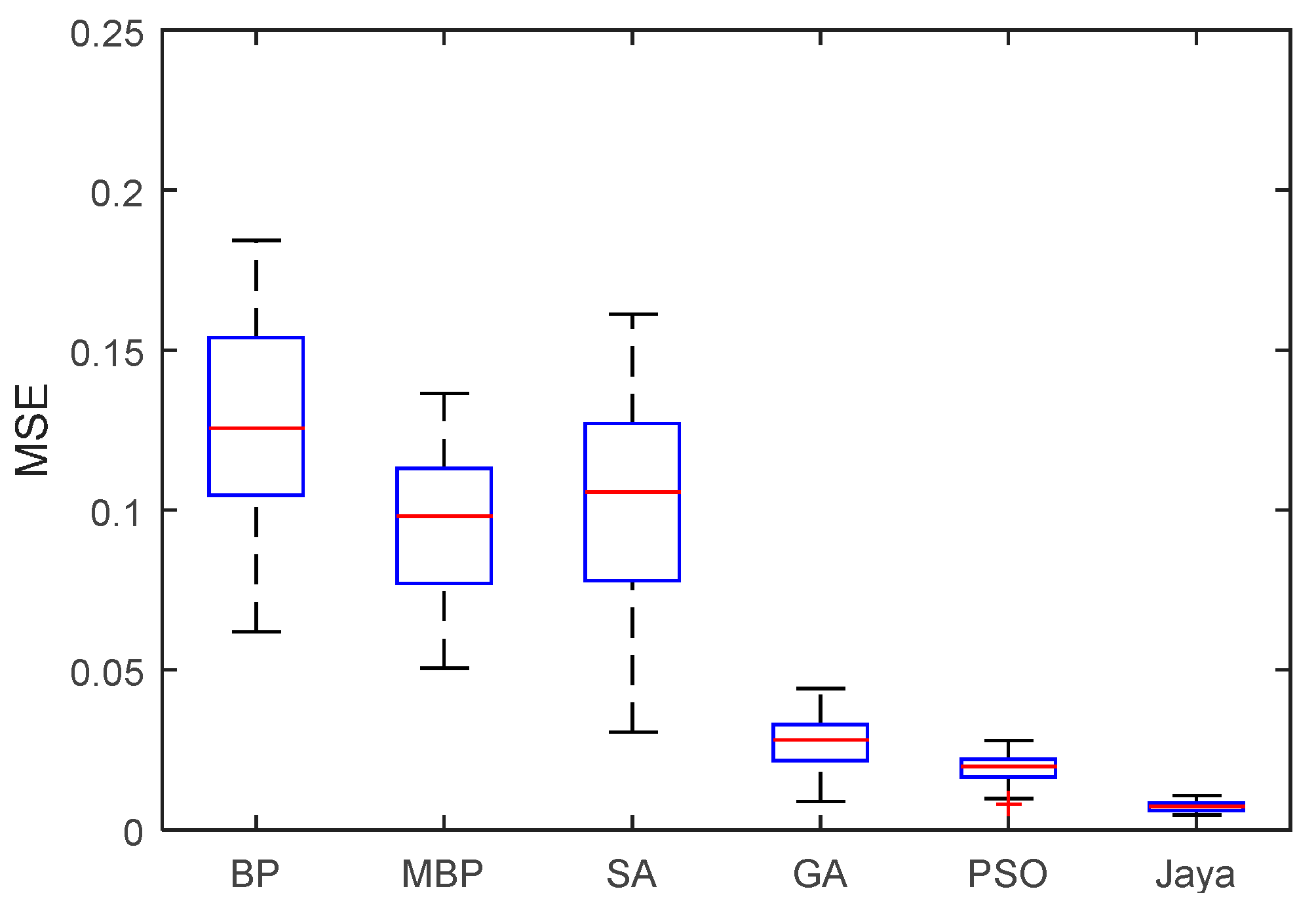
6.6. Training Comparison

Since RBF-KPCA obtains the least feature while yielding the largest cumulative variance, we believe its reduced features are more effective and will use it in the following experiments. The four reduced features are fed into FNN. Here, the number of input neurons is assigned with a value of four, since the number of features is four. The number of output neurons is set to three, since we need to classify from three classes: green, Oolong, and black. The number of hidden neurons is determined by cross-validation. Each time the training set was updated, we performed the grid search method to find the optimal number of hidden neurons.
We compared the Jaya method with different training methods: BP, MBP, GA, PSO, and SA. The maximum iterative epochs (MIEs) of all approaches are determined as 1000, since this value is rather large for such a small network. Actually, some approaches will converge at about 50 epochs. Hence, Figure 10 shows the ability to converge to a global optimal point. The populations are all set to 20. The ASPs of each algorithm were obtained by trial-and-error approach. Their values are listed in Table 4. The average and standard deviation (SD) of MSEs are shown in Figure 10, and their detailed data is shown in Table 5.
Table 5 shows that Jaya can find the least averaged MSE among all approaches. It achieves 0.0072 mean MSE, less than BP of 0.1242, MBP of 0.0939, SA of 0.1043, GA of 0.0266, and PSO of 0.0197. This again validates the superiority of Jaya. The reason may stem from that other algorithms may have a bad performance if the ASPs are not tuned well, while Jaya does not need to tune ASPs. Since Jaya has shown more superior performances than other approaches, we will use Jaya as the default approach for training FNN.

6.7. Feature Comparison

We compared three types of features: (1) only CH; (2) only FRFE; and (3) CH with FRFE, then reduced by KPCA. Classifiers were all set to Jaya-FNN. The measure was chosen as average sensitivity rate (ASR) based on a 10 × 10-fold SCV. The ASR is defined as the average value of sensitivity rate of 10 runs over the 10 validation folds. Table 6 lists the feature comparison results.
Table 6 shows that 64 CH yields ASRs of 94.7% ± 0.4%, 96.3% ± 0.5%, and 95.4% ± 0.5% over green, Oolong, and black tea, respectively. The 25 FRFE yields ASRs of 95.3% ± 0.3%, 98.2% ± 0.4%, and 96.6% ± 0.4% over green, Oolong, and black tea, respectively. Finally, their combination reduced to four PCs yields the largest ASRs of 97.3% ± 0.4%, 98.9% ± 0.3%, and 97.6% ± 0.3% over green, Oolong, and black tea, respectively. The results demonstrate that the combined feature performs better than single feature set, hence, the combination strategy is effective. Besides, the FRFE gives better results than CH, which suggests that the fractional features are more suitable to identify tea categories than color features.

6.8. Comparison to State-of-the-Art Approaches

We compared the best feature (64 CH and 25 FRFE, then reduced to four PCs) and the best classifier (Jaya-FNN), with seven state-of-the-art approaches (SVM [15], BPNN [16], LDA [21], GNN [22], FSCABC-FNN [25], SVM + WTA [28], and FSVM + WTA [28]), on the basis of ASR of 10 × 10-fold SCV, which were used in reference [25,28]. Table 7 shows the comparison results. The overall ASR is defined as the average ASR of three categories of teas.
Table 7 shows that our approach achieves ASR of 97.3% ± 0.4% on green tea, 98.9% ± 0.3% on Oolong tea, and 97.6% ± 0.3% on black tea, respectively. The overall ASR is 97.9% ± 0.3%, ranking first among all algorithms. The second best algorithm is “FSVM + WTA” [28] with overall ASR of 97.77%. The third one is FSCABC-FNN [25] with overall ASR of 97.4%. The fourth one is SVM + WTA [28] with overall ASR of 97.23%. The GNN [22] method ranks fifth with overall ASR of 96.0%. The LDA [21] approach ranks sixth with overall ASR of 96.5%. Finally, the two worst algorithms, BPNN [16] and SVM [15], yield the least overall ASR of 95%.
In addition, our method only used four reduced features, less than BPNN [16] of eight, SVM [15] of five, LDA [21] of 11, GNN [22] of eight, FSCABC-FNN [25] of 14, and SVM + WTA [28] of five.

7. Conclusions

Our contributions cover the following points: (i) We introduced a novel feature—fractional Fourier entropy (FRFE)—and showed its effectiveness in extracting features for tea images; (ii) We proposed a novel classifier—Jaya-FNN—by combining feedforward neural network with Jaya algorithm; (iii) We demonstrated that our TCI system was better than seven state-of-the-art approaches in terms of overall ASR and, meanwhile, our system used the least features.
In the future, we will test other newly proposed feature-extraction methods, such as displacement field [58,59] and image moments [60]. We will try to improve the classification performance, by introducing new swarm intelligence methods to train FNN classifier, or by introducing newly proposed classifiers, such as variants of SVMs. Besides, our method may be applied to X-ray image, magnetic resonance image, Alzheimer’s disease images, and microglia image.

Acknowledgments

This paper was supported by the National Natural Science Foundation of China (NSFC) (51407095, 61503188), the Natural Science Foundation of Jiangsu Province (BK20150983, BK20150982, BK20150973, BK20151548), the Jiangsu Key Laboratory of 3D Printing Equipment and Manufacturing (BM2013006), the Key Supporting Science and Technology Program (Industry) of Jiangsu Province (BE2012201, BE2013012-2, BE2014009-3), the Program of Natural Science Research of Jiangsu Higher Education Institutions (15KJB470010, 15KJB510018, 15KJB510016, 13KJB460011, 14KJB480004, 14KJB520021), the Special Funds for Scientific and Technological Achievement Transformation Project in Jiangsu Province (BA2013058), the Nanjing Normal University Research Foundation for Talented Scholars (2013119XGQ0061, 2014119XGQ0080), and the Open Fund of Guangxi Key Laboratory of Manufacturing Systems and Advanced Manufacturing Technology (15-140-30-008K).

Author Contributions

Yudong Zhang and Xiaojun Yang designed the experiments; Carlo Cattani and Ravipudi Venkata Rao performed the experiments; Shuihua Wang and Preetha Phillips analyzed the results; Yudong Zhang and Shuihua Wang collected the materials; Yudong Zhang, Xiaojun Yang and Preetha Phillips wrote the paper. All authors have read and approved the final manuscript.

Conflicts of Interest

The authors declare no conflict of interest.

Abbreviations

The following abbreviations are used in this manuscript:
AbbreviationDefinition
(BP)(F)NN(back-propagation) (feed-forward) neural network
(F)(B)L(Front) (Back) Lighting
ASPAlgorithm-specific parameter
ASRAverage sensitivity rate
CCDCharge-coupled device
CCPCommon controlling parameter
FNNFeed-forward neural network
FRFD/E/TFRactional Fourier domain/entropy/transform
FSCABCFitness-scaled Chaotic Artificial bee colony
FSVMFuzzy SVM
GNNGenetic neural-network
LDALinear discriminant analysis
NIRNear-infrared
OHLOne-hidden-layer
SCVStratified cross validation
SEShannon entropy
SVMSupport vector machine
TLBOTeaching-learning-based optimization
WPEWavelet packet entropy
WTAWinner-Takes-All

References

  1. Yang, C.S.; Landau, J.M. Effects of tea consumption on nutrition and health. J. Nutr. 2000, 130, 2409–2412. [Google Scholar] [PubMed]
  2. Ch Yiannakopoulou, E. Green tea catechins: Proposed mechanisms of action in breast cancer focusing on the interplay between survival and apoptosis. Anti-Cancer Agents Med. Chem. 2014, 14, 290–295. [Google Scholar] [CrossRef]
  3. Sironi, E.; Colombo, L.; Lompo, A.; Messa, M.; Bonanomi, M.; Regonesi, M.E.; Salmona, M.; Airoldi, C. Natural compounds against neurodegenerative diseases: Molecular characterization of the interaction of catechins from green tea with Aβ1-42, PrP106-126, and ataxin-3 oligomers. Chemistry 2014, 20, 13793–13800. [Google Scholar] [CrossRef] [PubMed]
  4. Miura, K.; Hughes, M.C.B.; Arovah, N.I.; van der Pols, J.C.; Green, A.C. Black tea consumption and risk of skin cancer: An 11-year prospective study. Nutr. Cancer 2015, 67, 1049–1055. [Google Scholar] [CrossRef] [PubMed]
  5. Qi, H.; Li, S.X. Dose-response meta-analysis on coffee, tea and caffeine consumption with risk of Parkinson’s disease. Geriatr. Gerontol. Int. 2014, 14, 430–439. [Google Scholar] [CrossRef] [PubMed]
  6. Gopalakrishna, R.; Fan, T.; Deng, R.; Rayudu, D.; Chen, Z.W.; Tzeng, W.S.; Gundimeda, U. Extracellular matrix components influence prostate tumor cell sensitivity to cancer-preventive agents selenium and green tea polyphenols. Cancer Res. 2014, 74. [Google Scholar] [CrossRef]
  7. Lim, H.J.; Shim, S.B.; Jee, S.W.; Lee, S.H.; Lim, C.J.; Hong, J.T.; Sheen, Y.Y.; Hwang, D.Y. Green tea catechin leads to global improvement among Alzheimer’s disease-related phenotypes in NSE/hAPP-C105 Tg mice. J. Nutr. Biochem. 2013, 24, 1302–1313. [Google Scholar] [CrossRef] [PubMed]
  8. Bohn, S.K.; Croft, K.D.; Burrows, S.; Puddey, I.B.; Mulder, T.P. J.; Fuchs, D.; Woodmand, R.J.; Hodgson, J.M. Effects of black tea on body composition and metabolic outcomes related to cardiovascular disease risk: A randomized controlled trial. Food Funct. 2014, 5, 1613–1620. [Google Scholar] [CrossRef] [PubMed]
  9. Hajiaghaalipour, F.; Kanthimathi, M.S.; Sanusi, J.; Rajarajeswaran, J. White tea (Camellia sinensis) inhibits proliferation of the colon cancer cell line, HT-29, activates caspases and protects DNA of normal cells against oxidative damage. Food Chem. 2015, 169, 401–410. [Google Scholar] [CrossRef] [PubMed]
  10. Horanni, R.; Engelhardt, U.H. Determination of amino acids in white, green, black, oolong, pu-erh teas and tea products. J. Food Compos. Anal. 2013, 31, 94–100. [Google Scholar] [CrossRef]
  11. DeCost, B.L.; Holm, E.A. A computer vision approach for automated analysis and classification of microstructural image data. Comput. Mater. Sci. 2015, 110, 126–133. [Google Scholar] [CrossRef]
  12. Gomez, M.J.; Garcia, F.; Martin, D.; de la Escalera, A.; Armingol, J.M. Intelligent surveillance of indoor environments based on computer vision and 3D point cloud fusion. Expert Syst. Appl. 2015, 42, 8156–8171. [Google Scholar] [CrossRef]
  13. Wang, S.; Feng, M.M.; Li, Y.; Zhang, Y.; Han, L.; Wu, J.; Du, S.D. Detection of dendritic spines using wavelet-based conditional symmetric analysis and regularized morphological shared-weight neural networks. Comput. Math. Methods Med. 2015. [Google Scholar] [CrossRef] [PubMed]
  14. Zhao, J.W.; Chen, Q.S.; Huang, X.Y.; Fang, C.H. Qualitative identification of tea categories by near infrared spectroscopy and support vector machine. J. Pharm. Biomed. Anal. 2006, 41, 1198–1204. [Google Scholar] [CrossRef] [PubMed]
  15. Chen, Q.S.; Zhao, J.W.; Fang, C.H.; Wang, D.M. Feasibility study on identification of green, black and Oolong teas using near-infrared reflectance spectroscopy based on support vector machine (SVM). Spectrochim. Acta A Mol. Biomol. Spectrosc. 2007, 66, 568–574. [Google Scholar] [CrossRef] [PubMed]
  16. Herrador, M.A.; Gonzalez, A.G. Pattern recognition procedures for differentiation of green, black and Oolong teas according to their metal content from inductively coupled plasma atomic emission spectrometry. Talanta 2001, 53, 1249–1257. [Google Scholar] [CrossRef]
  17. Chen, Q.S.; Liu, A.P.; Zhao, J.W.; Ouyang, Q. Classification of tea category using a portable electronic nose based on an odor imaging sensor array. J. Pharm. Biomed. Anal. 2013, 84, 77–89. [Google Scholar] [CrossRef] [PubMed]
  18. Szymczycha-Madeja, A.; Welna, M.; Pohl, P. Determination of essential and non-essential elements in green and black teas by FAAS and ICP OES simplified—Multivariate classification of different tea products. Microchem. J. 2015, 121, 122–129. [Google Scholar] [CrossRef]
  19. Liu, N.A.; Liang, Y.Z.; Bin, J.; Zhang, Z.M.; Huang, J.H.; Shu, R.X.; Yang, K. Classification of green and black teas by PCA and SVM analysis of cyclic voltammetric signals from metallic oxide-modified electrode. Food Anal. Meth. 2014, 7, 472–480. [Google Scholar] [CrossRef]
  20. Dai, Y.W.; Zhi, R.C.; Zhao, L.; Gao, H.Y.; Shi, B.L.; Wang, H.Y. Longjing tea quality classification by fusion of features collected from E-nose. Chemom. Intell. Lab. Syst. 2015, 144, 63–70. [Google Scholar] [CrossRef]
  21. Chen, Q.; Zhao, J.; Cai, J. Identification of tea varieties using computer vision. Trans. ASABE 2008, 51, 623–628. [Google Scholar] [CrossRef]
  22. Jian, W.; Xianyin, Z.; ShiPing, D. Identification and grading of tea using computer vision. Appl. Eng. Agric. 2010, 26, 639–645. [Google Scholar] [CrossRef]
  23. Laddi, A.; Sharma, S.; Kumar, A.; Kapur, P. Classification of tea grains based upon image texture feature analysis under different illumination conditions. J. Food Eng. 2013, 115, 226–231. [Google Scholar] [CrossRef]
  24. Gill, G.S.; Kumar, A.; Agarwal, R. Monitoring and grading of tea by computer vision—A review. J. Food Eng. 2011, 106, 13–19. [Google Scholar] [CrossRef]
  25. Zhang, Y.; Wang, S.; Ji, G.; Phillips, P. Fruit classification using computer vision and feedforward neural network. J. Food Eng. 2014, 143, 167–177. [Google Scholar] [CrossRef]
  26. Tang, Z.; Su, Y.C.; Er, M.J.; Qi, F.; Zhang, L.; Zhou, J.Y. A local binary pattern based texture descriptors for classification of tea leaves. Neurocomputing 2015, 168, 1011–1023. [Google Scholar] [CrossRef]
  27. Akar, O.; Gungor, O. Integrating multiple texture methods and NDVI to the Random Forest classification algorithm to detect tea and hazelnut plantation areas in northeast Turkey. Int. J. Remote Sens. 2015, 36, 442–464. [Google Scholar] [CrossRef]
  28. Wang, S.; Yang, X.; Zhang, Y.; Phillips, P.; Yang, J.; Yuan, T.F. Identification of green, oolong and black teas in China via wavelet packet entropy and fuzzy support vector machine. Entropy 2015, 17, 6663–6682. [Google Scholar] [CrossRef]
  29. Wang, S.; Zhang, Y.; Yang, X.J.; Sun, P.; Dong, Z.C.; Liu, A.J.; Yuan, T.F. Pathological brain detection by a novel image feature—Fractional Fourier entropy. Entropy 2015, 17, 8278–8296. [Google Scholar] [CrossRef]
  30. Rao, R.V. Jaya: A simple and new optimization algorithm for solving constrained and unconstrained optimization problems. Int. J. Ind. Eng. Comput. 2016, 7, 19–34. [Google Scholar]
  31. Tai, Y.H.; Chou, L.S.; Chiu, H.L. Gap-Type a-Si TFTs for Front Light Sensing Application. J. Disp. Technol. 2011, 7, 679–683. [Google Scholar] [CrossRef]
  32. Diniz, P.; Dantas, H.V.; Melo, K.D.T.; Barbosa, M.F.; Harding, D.P.; Nascimento, E.C.L.; Pistonesi, M.F.; Band, B.S.F.; Araujo, M.C.U. Using a simple digital camera and SPA-LDA modeling to screen teas. Anal. Methods 2012, 4, 2648–2652. [Google Scholar] [CrossRef]
  33. Yu, X.J.; Liu, K.S.; He, Y.; Wu, D. Color and texture classification of green tea using least squares support vector machine (LSSVM). Key Eng. Mater. 2011, 460–461, 774–779. [Google Scholar] [CrossRef]
  34. De Almeida, V.E.; da Costa, G.B.; Fernandes, D.D.D.; Diniz, P.; Brandao, D.; de Medeiros, A.C.D.; Veras, G. Using color histograms and SPA-LDA to classify bacteria. Anal. Bioanal. Chem. 2014, 406, 5989–5995. [Google Scholar] [CrossRef] [PubMed]
  35. Ajmera, P.K.; Holambe, R.S. Fractional Fourier transform based features for speaker recognition using support vector machine. Comput. Electr. Eng. 2013, 39, 550–557. [Google Scholar] [CrossRef]
  36. Machado, J.A.T. Matrix fractional systems. Commun. Nonlinear Sci. Numer. Simul. 2015, 25, 10–18. [Google Scholar] [CrossRef]
  37. Cagatay, N.D.; Datcu, M. FrFT-based scene classification of phase-gradient InSAR images and effective baseline dependence. IEEE Geosci. Remote Sens. Lett. 2015, 12, 1131–1135. [Google Scholar] [CrossRef]
  38. Bailey, D.H.; Swarztrauber, P.N. The fractional Fourier transform and applications. SIAM Rev. 1991, 33, 389–404. [Google Scholar] [CrossRef]
  39. Chen, S.F.; Wang, S.H.; Yang, J.F.; Phillips, P. Magnetic resonance brain image classification based on weighted-type fractional Fourier transform and nonparallel support vector machine. Int. J. Imaging Syst. Technol. 2015, 24, 317–327. [Google Scholar]
  40. Azoug, S.E.; Bouguezel, S. A non-linear preprocessing for opto-digital image encryption using multiple-parameter discrete fractional Fourier transform. Opt. Commun. 2016, 359, 85–94. [Google Scholar] [CrossRef]
  41. Machado, J.A.T. A fractional perspective to financial indices. Optimization 2014, 63, 1167–1179. [Google Scholar] [CrossRef]
  42. Yang, X.J.; Dong, Z.C.; Liu, G.; Phillips, P. Pathological brain detection in MRI scanning by wavelet packet Tsallis entropy and fuzzy support vector machine. SpringerPlus 2015, 4. [Google Scholar] [CrossRef]
  43. Llave, Y.A.; Hagiwara, T.; Sakiyama, T. Artificial neural network model for prediction of cold spot temperature in retort sterilization of starch-based foods. J. Food Eng. 2012, 109, 553–560. [Google Scholar] [CrossRef]
  44. Shojaee, S.A.; Hezave, A.Z.; Lashkarbolooki, M.; Shafipour, Z.S. Prediction of the binary density of the ionic liquids plus water using back-propagated feed forward artificial neural network. Chem. Ind. Chem. Eng. Q. 2014, 20, 325–338. [Google Scholar] [CrossRef]
  45. Karmakar, S.; Shrivastava, G.; Kowar, M.K. Impact of learning rate and momentum factor in the performance of back-propagation neural network to identify internal dynamics of chaotic motion. Kuwait J. Sci. 2014, 41, 151–174. [Google Scholar]
  46. Chandwani, V.; Agrawal, V.; Nagar, R. Modeling slump of ready mix concrete using genetic algorithms assisted training of Artificial Neural Networks. Expert Syst. Appl. 2015, 42, 885–893. [Google Scholar] [CrossRef]
  47. Manoochehri, M.; Kolahan, F. Integration of artificial neural network and simulated annealing algorithm to optimize deep drawing process. Int. J. Adv. Manuf. Technol. 2014, 73, 241–249. [Google Scholar] [CrossRef]
  48. Awan, S.M.; Aslam, M.; Khan, Z.A.; Saeed, H. An efficient model based on artificial bee colony optimization algorithm with Neural Networks for electric load forecasting. Neural Comput. Appl. 2014, 25, 1967–1978. [Google Scholar] [CrossRef]
  49. Momeni, E.; Armaghani, D.J.; Hajihassani, M.; Amin, M.F.M. Prediction of uniaxial compressive strength of rock samples using hybrid particle swarm optimization-based artificial neural networks. Measurement 2015, 60, 50–63. [Google Scholar] [CrossRef]
  50. Wang, S.; Ji, G.L.; Yang, J.Q.; Wu, J.G.; Wei, L. Fruit classification by wavelet-entropy and feedforward neural network trained by fitness-scaled chaotic ABC and biogeography-based optimization. Entropy 2015, 17, 5711–5728. [Google Scholar] [CrossRef]
  51. Yu, L.; Wang, S.Y.; Kai, K.K. Forecasting foreign exchange rates with an improved back-propagation learning algorithm with adaptive smoothing momentum terms. Front. Comput. Sci. China 2009, 3, 167–176. [Google Scholar] [CrossRef]
  52. Rao, R.V.; Savsani, V.J.; Vakharia, D.P. Teaching-learning-based optimization: A novel method for constrained mechanical design optimization problems. Comput. Aided Des. 2011, 43, 303–315. [Google Scholar] [CrossRef]
  53. Rao, R.V.; Savsani, V.J.; Balic, J. Teaching-learning-based optimization algorithm for unconstrained and constrained real-parameter optimization problems. Eng. Optim. 2012, 44, 1447–1462. [Google Scholar] [CrossRef]
  54. Dokeroglu, T. Hybrid teaching-learning-based optimization algorithms for the Quadratic Assignment Problem. Comput. Ind. Eng. 2015, 85, 86–101. [Google Scholar] [CrossRef]
  55. Gonzalez-Alvarez, D.L.; Vega-Rodriguez, M.A.; Rubio-Largo, A. Finding patterns in protein sequences by using a hybrid multiobjective teaching learning based optimization algorithm. IEEE ACM Trans. Comput. Biol. Bioinform. 2015, 12, 656–666. [Google Scholar] [CrossRef] [PubMed]
  56. Dede, T.; Togan, V. A teaching learning based optimization for truss structures with frequency constraints. Struct. Eng. Mech. 2015, 53, 833–845. [Google Scholar] [CrossRef]
  57. Rao, R.V.; Patel, V. An improved teaching-learning-based optimization algorithm for solving unconstrained optimization problems. Sci. Iran. 2013, 20, 710–720. [Google Scholar] [CrossRef]
  58. Zhang, Y.D. Detection of Alzheimer’s disease by displacement field and machine learning. PeerJ 2015, 3, e1251. [Google Scholar] [CrossRef] [PubMed]
  59. Wang, S.; Zhang, Y.; Liu, G.; Phillips, P.; Yuan, T.F. Detection of Alzheimer’s Disease by Three-Dimensional Displacement Field Estimation in Structural Magnetic Resonance Imaging. J. Alzheimer’s Dis. 2015, 50, 233–248. [Google Scholar] [CrossRef] [PubMed]
  60. Zhang, Y.; Wang, S.; Sun, P.; Phillips, P. Pathological Brain Detection based on wavelet entropy and Hu moment invariants. Bio-Med. Mater. Eng. 2015, 26, S1283–S1290. [Google Scholar] [CrossRef] [PubMed]
Figure 1. Tea image acquiring system.
Entropy 18 00077 g001
Figure 2. Fractional Fourier transform (FRFT) of tri(t).
Entropy 18 00077 g002
Figure 3. Flowchart of feature processing.
Entropy 18 00077 g003
Figure 4. Diagram of one-hidden-layer feedforward neural network (OHL-FNN).
Entropy 18 00077 g004
Figure 5. Diagram of Jaya algorithm.
Entropy 18 00077 g005
Figure 6. Color histogram of green, Oolong, and black tea [28].
Entropy 18 00077 g006
Figure 7. 2D-FRFT of an image of Oolong tea.
Entropy 18 00077 g007
Figure 8. Comparing KPCA with PCA over 3D simulation data. (a) 3D Simulation Data; (b) PCA Result with 2 PCs; (c) POL-KPCA with 2 PCs; (d) RBF-KPCA with 2 PCs.
Entropy 18 00077 g008
Figure 9. Curve of accumulated variance versus principal component number.
Entropy 18 00077 g009
Figure 10. Comparison of different FNN training methods.
Entropy 18 00077 g010
Table 1. Three main tea in China.
Tea CategoryWiltedBruisedOxidized
GreenNoNoNo
OolongYesYesPartially
BlackYesNoYes
Table 2. Tea sample settings.
Category *#Origins
G100Guizhou; Henan; Anhui; Jiangxi; Jiangsu; Zhejiang
B100Yunnan; Fujian; Hunan; Hubei
O100Guangdong; Fujian
* G = Green, B = Black, O = Oolong. # = Number.
Table 3. Statistics of fractional Fourier entropy (FRFE) of different tea (The top, middle, and bottom digits represents the FRFE values of green, Oolong, and black teas, respectively).
Angles0.60.70.80.91.0
0.67.35 + 0.107.15 + 0.066.82 + 0.046.56 + 0.036.32 + 0.09
7.31 + 0.097.12 + 0.086.80 + 0.066.50 + 0.086.24 + 0.17
6.94 + 0.116.81 + 0.106.62 + 0.096.39 + 0.045.85 + 0.11
0.77.15 + 0.066.91 + 0.046.61 + 0.046.48 + 0.056.31 + 0.08
7.12 + 0.086.88 + 0.066.57 + 0.076.40 + 0.106.22 + 0.17
6.80 + 0.106.67 + 0.096.47 + 0.076.23 + 0.045.85 + 0.10
0.86.80 + 0.046.60 + 0.046.41 + 0.046.39 + 0.076.29 + 0.08
6.75 + 0.066.54 + 0.076.31 + 0.096.28 + 0.116.18 + 0.16
6.60 + 0.086.45 + 0.076.22 + 0.046.05 + 0.055.82 + 0.09
0.96.55 + 0.036.47 + 0.056.38 + 0.076.40 + 0.086.29 + 0.08
6.47 + 0.096.37 + 0.106.28 + 0.126.28 + 0.116.17 + 0.16
6.38 + 0.056.23 + 0.046.06 + 0.056.00 + 0.075.82 + 0.09
1.06.28 + 0.086.27 + 0.086.26 + 0.086.26 + 0.086.21 + 0.08
6.17 + 0.166.16 + 0.156.14 + 0.156.13 + 0.156.08 + 0.15
5.78 + 0.085.78 + 0.095.76 + 0.085.77 + 0.085.73 + 0.09
Table 4. Parameters obtained by trial-and-error.
AlgorithmCCP
AllMIE = 1000, Population = 20, RT = 50
AlgorithmASP
BPLR = 0.01
MBPLR = 0.01, MC = 0.9
PSOMV = 1, IW = 0.5, AC = 1
SATDF = “Exp”, IT = 100, FT = 0
GACP = 0.8, MP = 0.1
JayaNo ASPs
(MIE = Maximum Iterative Epoch, RT = Run Times, LR = Learning Rate, MC = Momentum Constant, CP = Crossover Probability, MP = Mutation Probability, TDF = Temperature Decrease Function, IT = 100, FT = Final Temperature, MV = Maximal Velocity, IW = Initial Weight, AC = Acceleration Coefficient).
Table 5. Result details of training methods.
Proposed MethodMeanSD
BP0.12420.0269
MBP0.09390.0228
SA0.10430.0317
GA0.02660.0105
PSO0.01970.0040
Jaya0.00720.0015
Table 6. Feature Comparison.
FeatureGreenOolongBlack
64 CH94.7% ± 0.4%96.3% ± 0.5%95.4% ± 0.5%
25 FRFE95.3% ± 0.3%98.2% ± 0.4%96.6% ± 0.4%
(64 CH and 25 FRFE) reduced to 4 PCs97.3% ± 0.4%98.9% ± 0.3%97.6% ± 0.3%
Table 7. Average sensitivity rate (ASR) over a 10 × 10-fold stratified cross validation (SCV).
Existing Approaches
Original FeaturesReduced Feature #Classification MethodGreenOolongBlackOverallRank
3735 spectrum5SVM [15]90%100%95%95%7
8 metal8BPNN [16]95%7
12 color, 12 texture11LDA [21]96.7%92.3%98.5%95.8%6
2 color, 6 shape8GNN [22]95.8%94.4%97.9%96.0%5
64 CH, 7 texture, 8 shape14FSCABC-FNN [25]98.1%97.7%96.4%97.4%3
64 CH, 16 WPE5SVM + WTA [28]95.7%98.1%97.9%97.23%4
64 CH, 16 WPE5FSVM + WTA [28]96.2%98.8%98.3%97.77%2
Proposed Approaches
64 CH, 25 FRFE4Jaya-FNN97.3% ± 0.4%98.9% ± 0.3%97.6% ± 0.3%97.9% ± 0.3%1
# = Number.

