
New Lagrange Multipliers for the Blind Adaptive Deconvolution Problem Applicable for the Noisy Case

Abstract
:1. Introduction
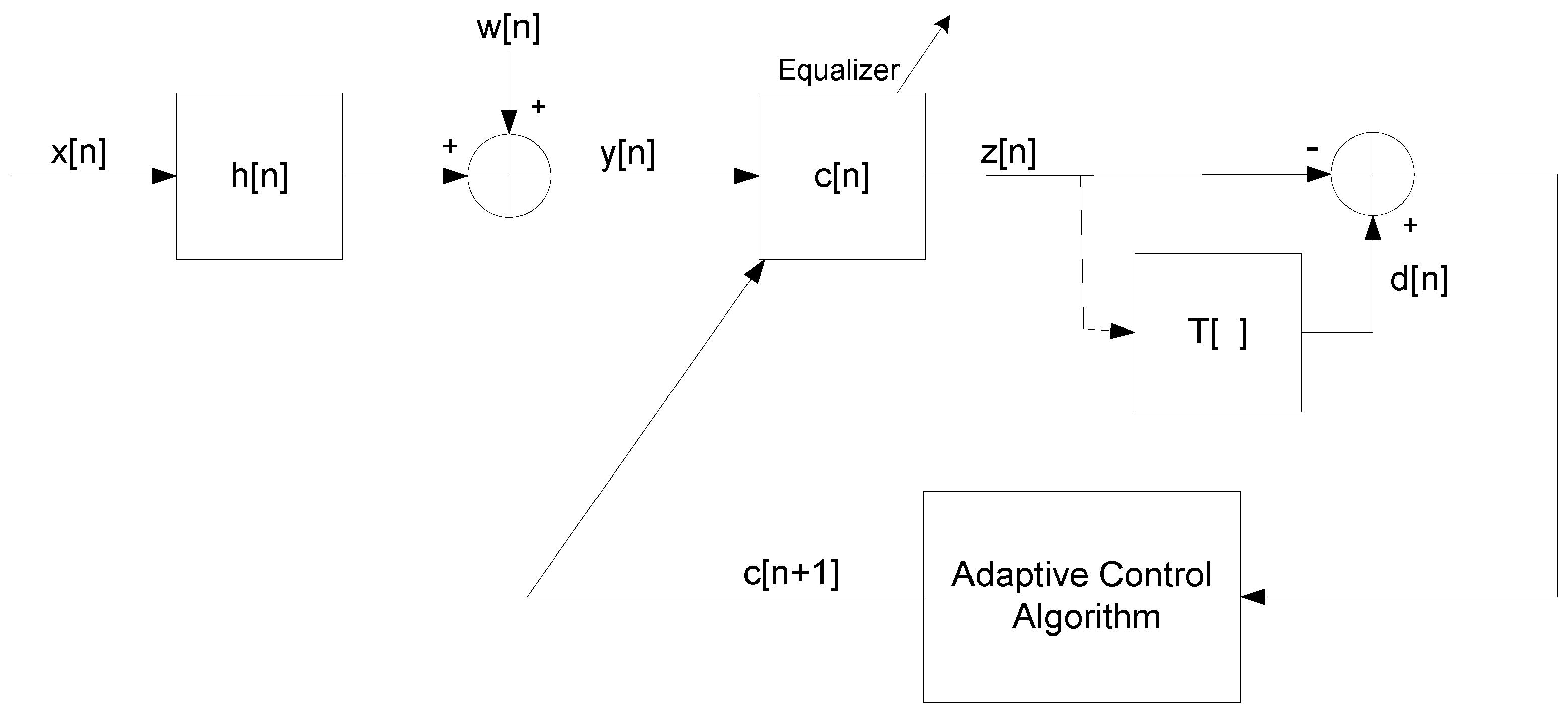
2. System Description
- The input sequence can be written as , where and are the real and imaginary parts of , respectively. We assume that and are independent and that , where stands for the expectation operation.
- The unknown channel is a possibly non-minimum phase linear time-invariant filter in which the transfer function has no “deep zeros”, namely the zeros lie sufficiently far from the unit circle.
- The filter is a tap-delay line.
- The channel noise is an additive Gaussian white noise.
- The function is a memoryless nonlinear function that satisfies the additivity condition: , where , are the real and imaginary parts of the equalized output, respectively.
3. The New Lagrange Multipliers
- The convolutional noise is a zero mean, white Gaussian process with variance (where is the conjugate operation on ).
- The source signal is an independent non-Gaussian signal with known variance and higher moments.
- The convolutional noise and the source signal are independent.
- The convolutional noise power is sufficiently low.
3.1. Closed-Form Approximated Expressions for , and
3.2. Closed-Form Approximated Expression for the MSE
3.3. Closed-Form Approximated Expressions for and
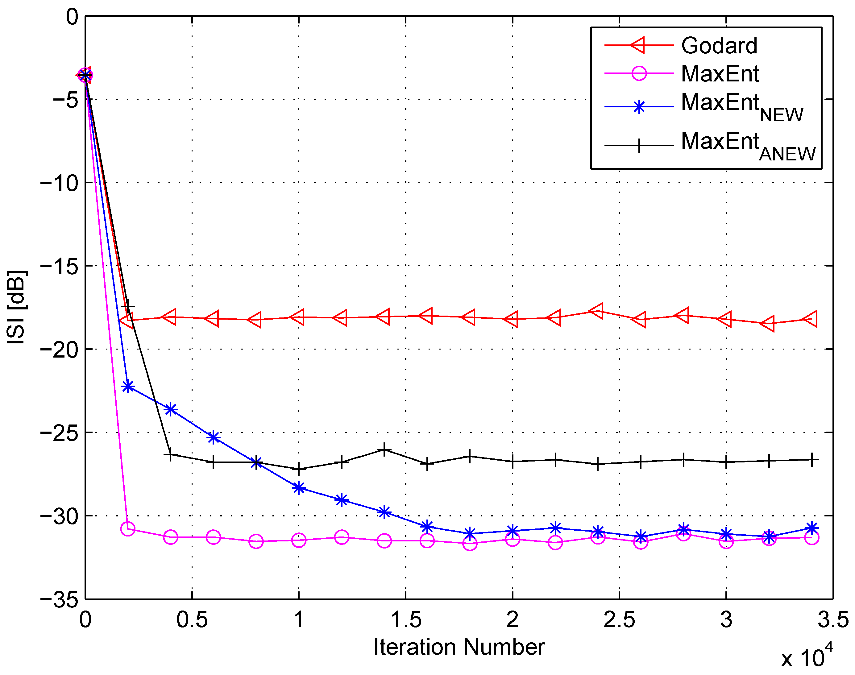
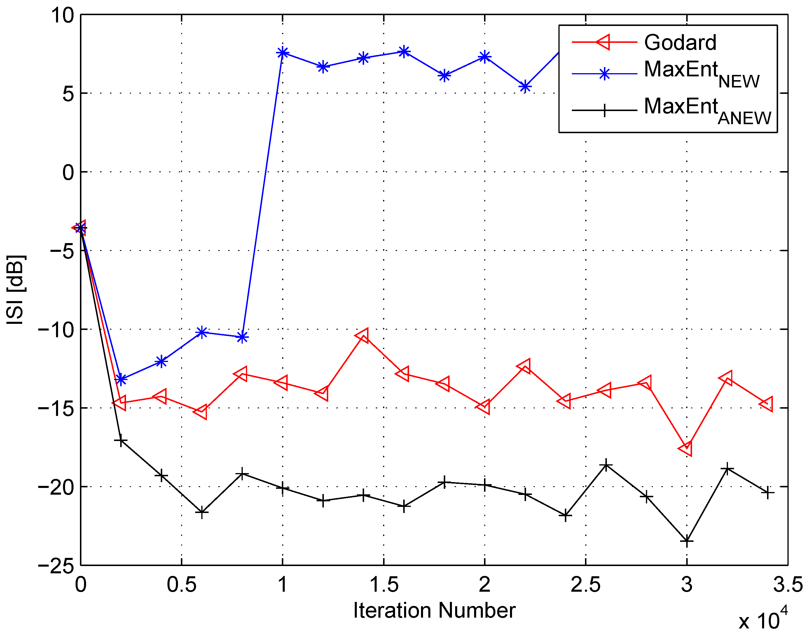
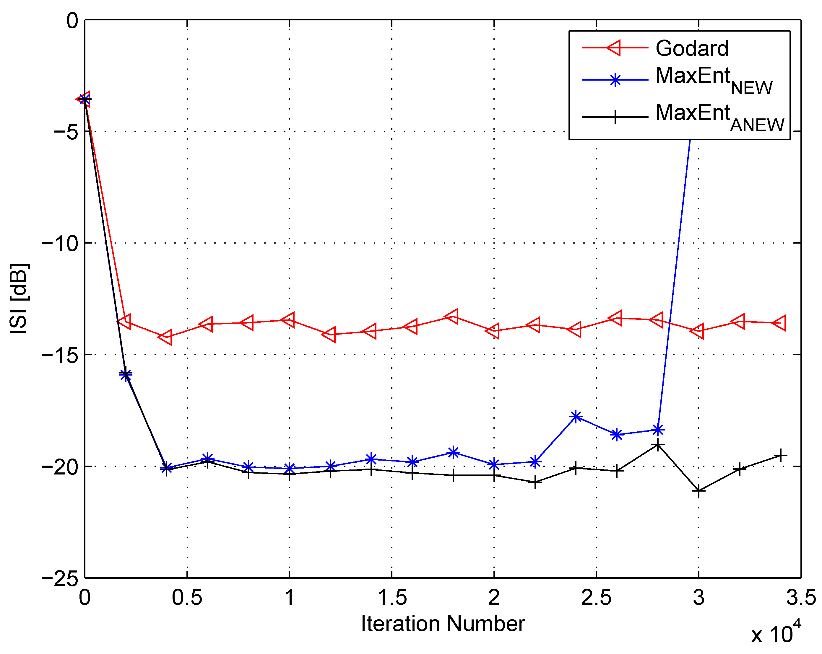
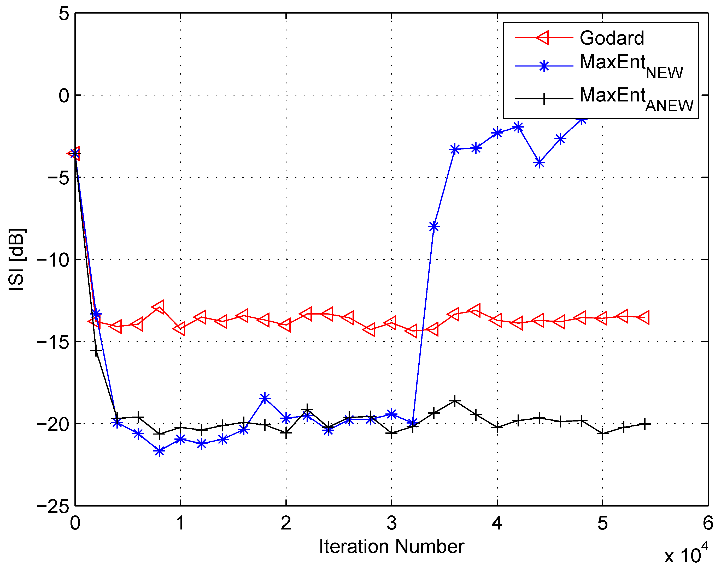
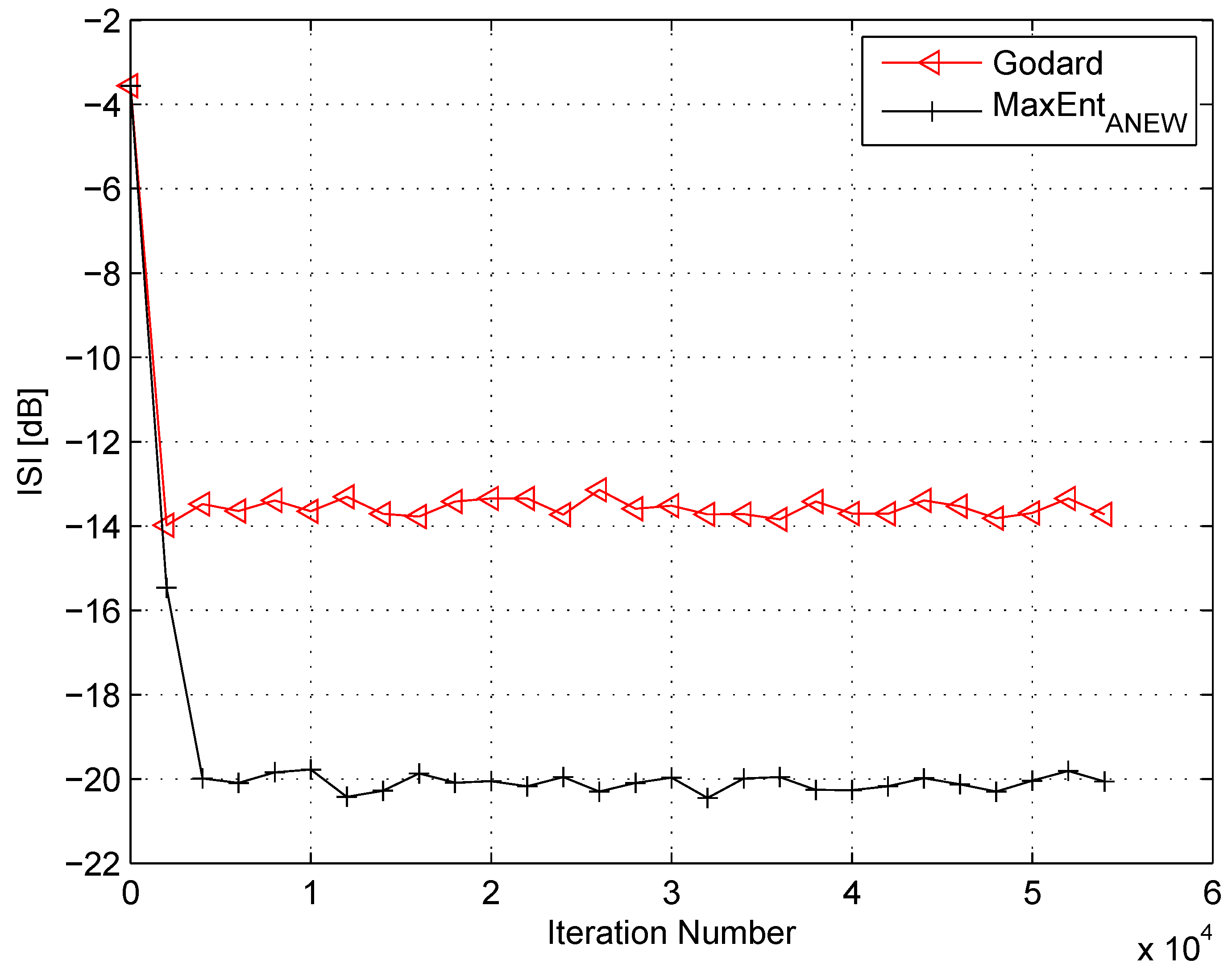
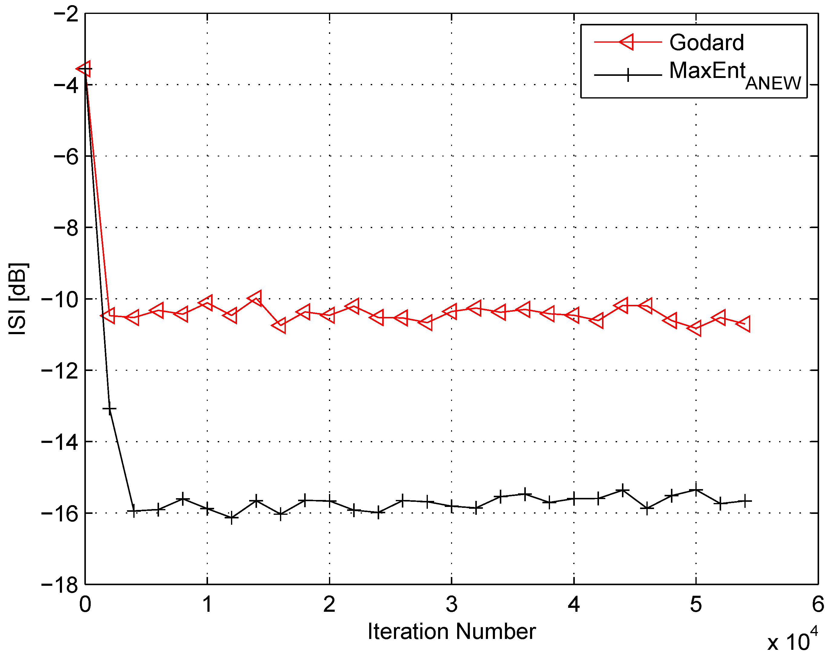
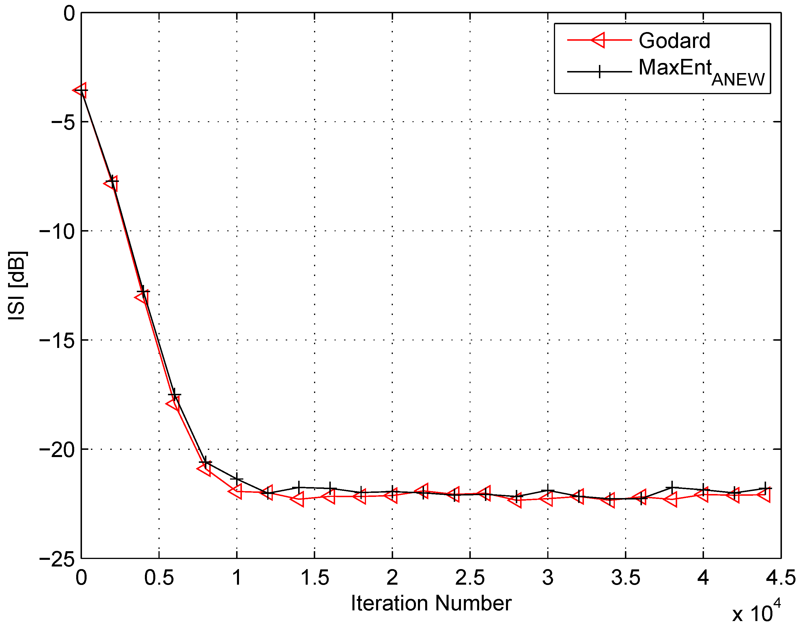
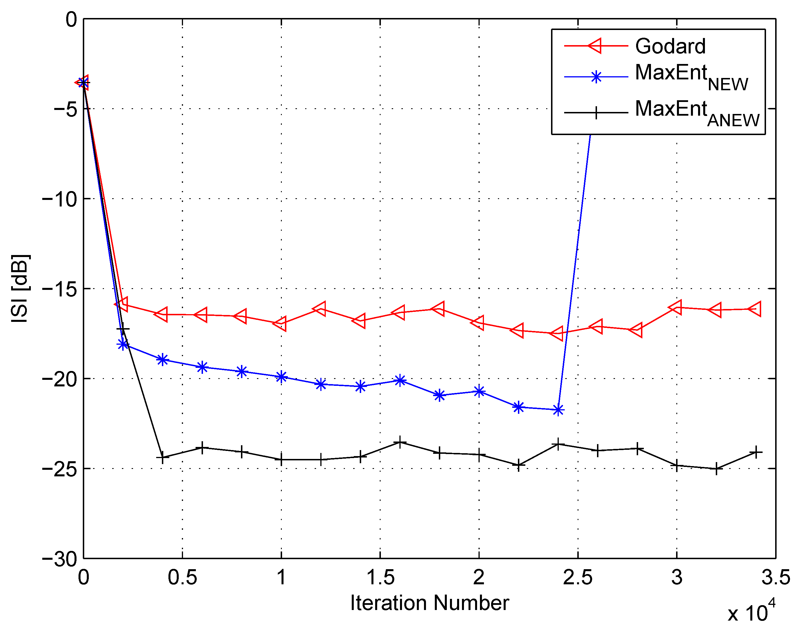
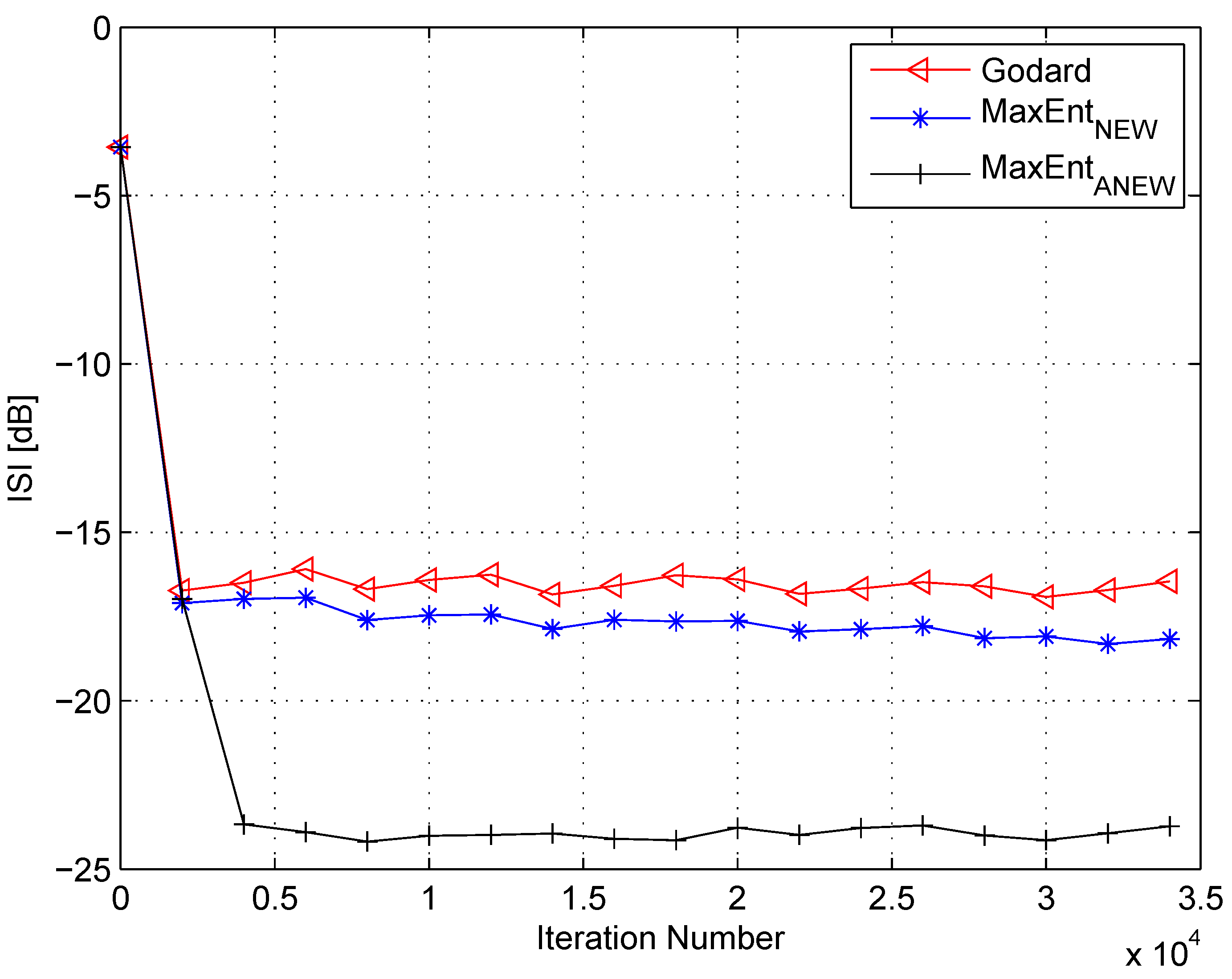
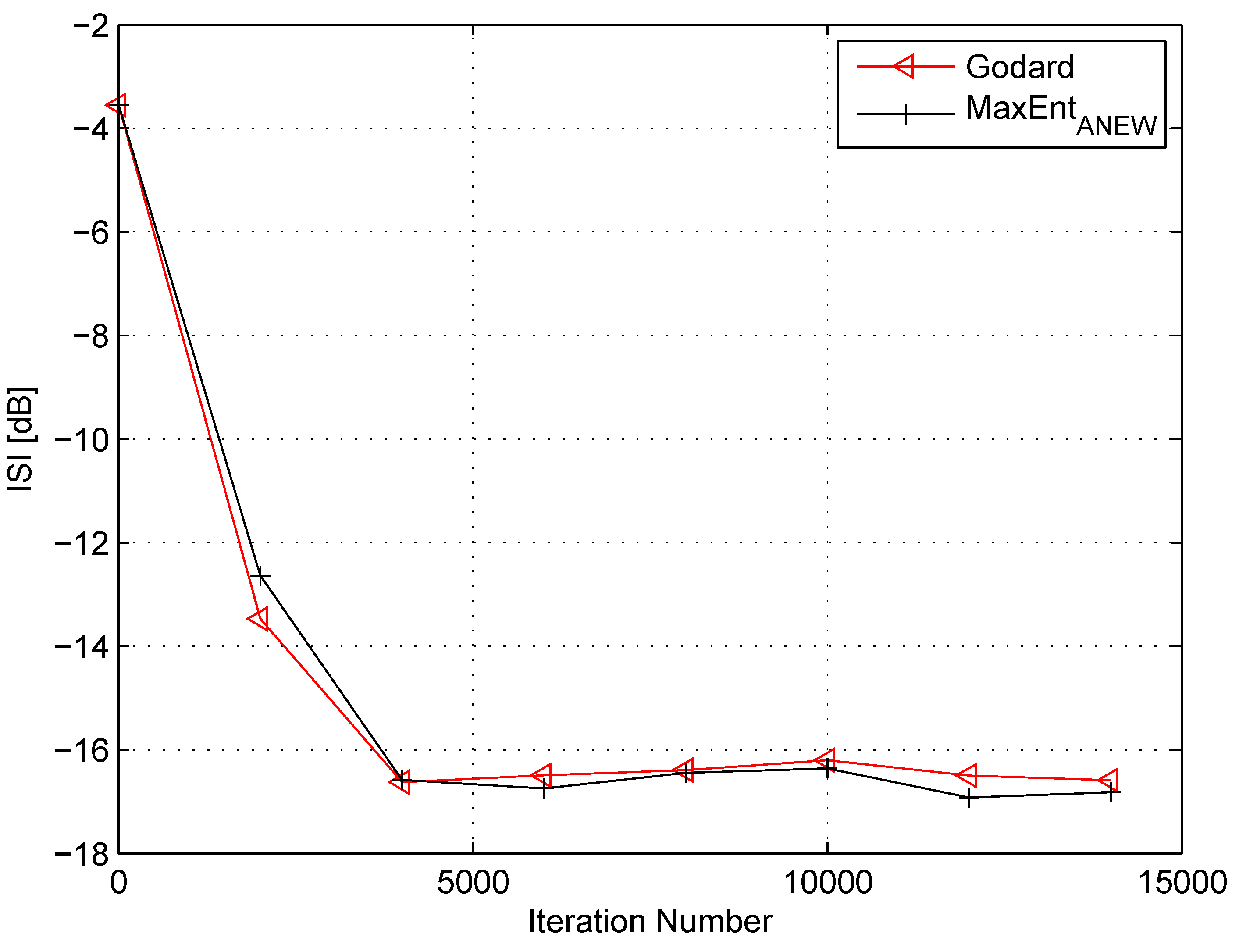
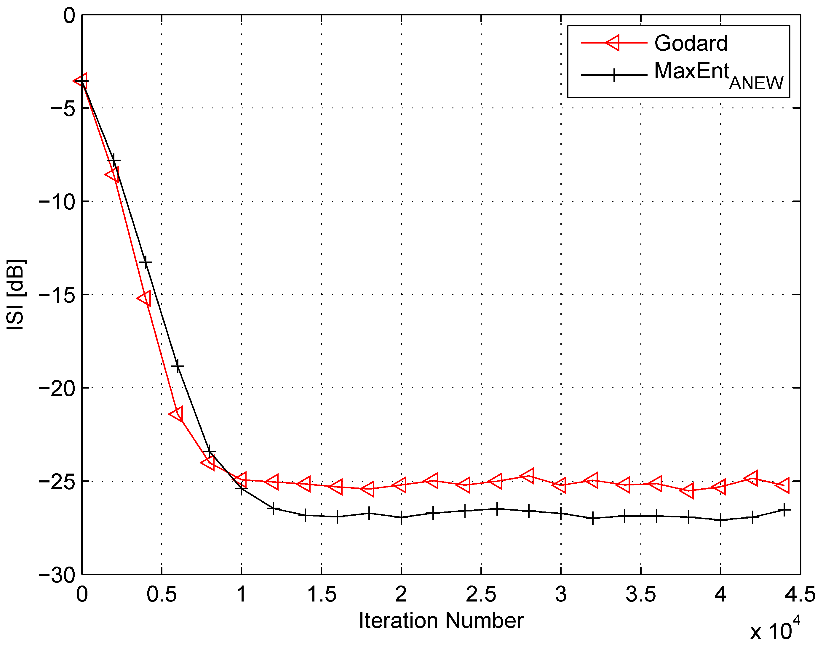
4. Simulation
5. Conclusions
Acknowledgments
Conflicts of Interest
References
- Shalvi, O.; Weinstein, E. New criteria for blind deconvolution of non-minimum phase systems (channels). IEEE Trans. Inf. Theory 1990, 36, 312–321. [Google Scholar] [CrossRef]
- Johnson, R.C.; Schniter, P.; Endres, T.J.; Behm, J.D.; Brown, D.R.; Casas, R.A. Blind Equalization Using the Constant Modulus Criterion: A Review. Proc. IEEE 1998, 86, 1927–1950. [Google Scholar] [CrossRef]
- Wiggins, R.A. Minimum entropy deconvolution. Geoexploration 1978, 16, 21–35. [Google Scholar] [CrossRef]
- Kazemi, N.; Sacchi, M.D. Sparse multichannel blind deconvolution. Geophysics 2014, 79, V143–V152. [Google Scholar] [CrossRef]
- Guitton, A.; Claerbout, J. Nonminimum phase deconvolution in the log domain: A sparse inversion approach. Geophysics 2015, 80, WD11–WD18. [Google Scholar] [CrossRef]
- Silva, M.T.M.; Arenas-Garcia, J. A Soft-Switching Blind Equalization Scheme via Convex Combination of Adaptive Filters. IEEE Trans. Signal Process. 2013, 61, 1171–1182. [Google Scholar] [CrossRef]
- Mitra, R.; Singh, S.; Mishra, A. Improved multi-stage clustering-based blind equalisation. IET Commun. 2011, 5, 1255–1261. [Google Scholar] [CrossRef]
- Gul, M.M.U.; Sheikh, S.A. Design and implementation of a blind adaptive equalizer using Frequency Domain Square Contour Algorithm. Digit. Signal Process. 2010, 20, 1697–1710. [Google Scholar]
- Sheikh, S.A.; Fan, P. New Blind Equalization techniques based on improved square contour algorithm. Digit. Signal Process. 2008, 18, 680–693. [Google Scholar] [CrossRef]
- Thaiupathump, T.; He, L.; Kassam, S.A. Square contour algorithm for blind equalization of QAM signals. Signal Process. 2006, 86, 3357–3370. [Google Scholar] [CrossRef]
- Sharma, V.; Raj, V.N. Convergence and performance analysis of Godard family and multimodulus algorithms for blind equalization. IEEE Trans. Signal Process. 2005, 53, 1520–1533. [Google Scholar] [CrossRef]
- Yuan, J.T.; Lin, T.C. Equalization and Carrier Phase Recovery of CMA and MMA in BlindAdaptive Receivers. IEEE Trans. Signal Process. 2010, 58, 3206–3217. [Google Scholar] [CrossRef]
- Yuan, J.T.; Tsai, K.D. Analysis of the multimodulus blind equalization algorithm in QAM communication systems. IEEE Trans. Commun. 2005, 53, 1427–1431. [Google Scholar] [CrossRef]
- Wu, H.C.; Wu, Y.; Principe, J.C.; Wang, X. Robust switching blind equalizer for wireless cognitive receivers. IEEE Trans. Wirel. Commun. 2008, 7, 1461–1465. [Google Scholar]
- Kundur, D.; Hatzinakos, D. A novel blind deconvolution scheme for image restoration using recursive filtering. IEEE Trans. Signal Process. 1998, 46, 375–390. [Google Scholar] [CrossRef]
- Likas, C.L.; Galatsanos, N.P. A variational approach for Bayesian blind image deconvolution. IEEE Trans. Signal Process. 2004, 52, 2222–2233. [Google Scholar] [CrossRef]
- Li, D.; Mersereau, R.M.; Simske, S. Blind Image Deconvolution Through Support Vector Regression. IEEE Trans. Neural Netw. 2007, 18, 931–935. [Google Scholar] [CrossRef] [PubMed]
- Amizic, B.; Spinoulas, L.; Molina, R.; Katsaggelos, A.K. Compressive Blind Image Deconvolution. IEEE Trans. Image Process. 2013, 22, 3994–4006. [Google Scholar] [CrossRef] [PubMed]
- Tzikas, D.G.; Likas, C.L.; Galatsanos, N.P. Variational Bayesian Sparse Kernel-Based Blind Image Deconvolution With Student’s-t Priors. IEEE Trans. Image Process. 2009, 18, 753–764. [Google Scholar] [CrossRef] [PubMed]
- Pinchas, M.; Bobrovsky, B.Z. A Maximum Entropy approach for blind deconvolution. Signal Process. 2006, 86, 2913–2931. [Google Scholar] [CrossRef]
- Feng, C.; Chi, C. Performance of cumulant based inverse filters for blind deconvolution. IEEE Trans. Signal Process. 1999, 47, 1922–1935. [Google Scholar] [CrossRef]
- Abrar, S.; Nandi, A.S. Blind Equalization of Square-QAM Signals: A Multimodulus Approach. IEEE Trans. Commun. 2010, 58, 1674–1685. [Google Scholar] [CrossRef]
- Vanka, R.N.; Murty, S.B.; Mouli, B.C. Performance comparison of supervised and unsupervised/blind equalization algorithms for QAM transmitted constellations. In Proceedings of 2014 International Conference on Signal Processing and Integrated Networks (SPIN), Noida, India, 20–21 February 2014.
- Ram Babu, T.; Kumar, P.R. Blind Channel Equalization Using CMA Algorithm. In Proceedings of 2009 International Conference on Advances in Recent Technologies in Communication and Computing (ARTCom 09), Kottayam, India, 27–28 October 2009.
- Qin, Q.; Huahua, L.; Tingyao, J. A new study on VCMA-based blind equalization for underwater acoustic communications. In Proceedings of 2013 International Conference on Mechatronic Sciences, Electric Engineering and Computer (MEC), Shengyang, China, 20–22 December 2013.
- Wang, J.; Huang, H.; Zhang, C.; Guan, J. A Study of the Blind Equalization in the Underwater Communication. In Proceedings of WRI Global Congress on Intelligent Systems, GCIS ’09, Xiamen, China, 19–21 May 2009.
- Miranda, M.D.; Silva, M.T.M.; Nascimento, V.H. Avoiding Divergence in the Shalvi Weinstein Algorithm. IEEE Trans. Signal Process. 2008, 56, 5403–5413. [Google Scholar] [CrossRef]
- Samarasinghe, P.D.; Kennedy, R.A. Minimum Kurtosis CMA Deconvolution for Blind Image Restoration. In Proceedings of the 4th International Conference on Information and Automation for Sustainability, ICIAFS 2008, Colombo, Sri Lanka, 12–14 December 2008.
- Fijalkow, I.; Touzni, A.; Treichler, J.R. Fractionally-Spaced Equalization using CMA: Robustness to Channel Noise and Lack of Disparity. IEEE Trans. Signal Process. 1997, 45, 56–66. [Google Scholar] [CrossRef]
- Fijalkow, I.; Manlove, C.E.; Johnson, C.R. Adaptive Fractionally Spaced Blind CMA Equalization: Excess MSE. IEEE Trans. Signal Process. 1998, 46, 227–231. [Google Scholar] [CrossRef]
- Moazzen, I.; Doost-Hoseini, A.M.; Omidi, M.J. A novel blind frequency domain equalizer for SIMO systems. In Proceedings of Wireless Communications and Signal Processing, WCSP, Nanjing, China, 13–15 November 2009.
- Peng, D.; Xiang, Y.; Yi, Z.; Yu, S. CM-Based Blind Equalization of Time-Varying SIMO-FIR Channel With Single Pulsation Estimation. IEEE Trans. Veh. Technol. 2011, 60, 2410–2415. [Google Scholar] [CrossRef]
- Coskun, A.; Kale, I. Blind Multidimensional Matched Filtering Techniques for Single Input Multiple Output Communications. IEEE Trans. Instrum. Meas. 2010, 59, 1056–1064. [Google Scholar] [CrossRef]
- Romano, J.M.T.; Attux, R.; Cavalcante, C.C.; Suyama, R. Unsupervised Signal Processing: Channel Equalization and Source Separation; CRC Press: Boca Raton, FL, USA, 2010. [Google Scholar]
- Chen, S.; Wolfgang, A.; Hanzo, L. Constant Modulus Algorithm Aided Soft Decision Directed Scheme for Blind Space-Time Equalization of SIMO Channels. Signal Process. 2007, 87, 2587–2599. [Google Scholar] [CrossRef]
- Pinchas, M. Two Blind Adaptive Equalizers Connected in Series for Equalization Performance Improvement. J. Signal Inf. Process. 2013, 4, 64–71. [Google Scholar] [CrossRef]
- Nikias, C.L.; Petropulu, A.P. (Eds.) Higher-Order Spectra Analysis a Nonlinear Signal Processing Framework; Prentice-Hall: Enlewood Cliffs, NJ, USA, 1993; pp. 419–425.
- Haykin, S. Adaptive Filter Theory. In Blind Deconvolution; Haykin, S., Ed.; Prentice-Hall: Englewood Cliffs, NJ, USA, 1991. [Google Scholar]
- Godard, D.N. Self recovering equalization and carrier tracking in two-dimenional data communication system. IEEE Trans. Commun. 1980, 28, 1867–1875. [Google Scholar] [CrossRef]
- Lazaro, M.; Santamaria, I.; Erdogmus, D.; Hild, K.E.; Pantaleon, C.; Principe, J.C. Stochastic blind equalization based on pdf fitting using parzen estimator. IEEE Trans. Signal Process. 2005, 53, 696–704. [Google Scholar] [CrossRef]
- Sato, Y. A method of self-recovering equalization for multilevel amplitude-modulation systems. IEEE Trans. Commun. 1975, 23, 679–682. [Google Scholar] [CrossRef]
- Beasley, A.; Cole-Rhodes, A. Performance of an adaptive blind equalizer for QAM signals. In Proceedings of IEEE Military Communications Conference, MILCOM 2005, Atlantic City, NJ, USA, 17–20 October 2015.
- Alaghbari, K.A.A.; Tan, A.W.C.; Lim, H.S. Cost function of blind channel equalization. In Proceedings of the 4th International Conference on Intelligent and Advanced Systems (ICIAS), Kuala Lumpur, Malaysia, 12–14 June 2012.
- Daas, A.; Hadef, M.; Weiss, S. Adaptive blind multiuser equalizer based on pdf matching. In Proceedings of the International Conference on Telecommunications, ICT ’09, Marrakech, Morocco, 25–27 May 2009.
- Giunta, G.; Benedetto, F. A signal processing algorithm for multi-constant modulus equalization. In Proceedings of the 36th International Conference on Telecommunications and Signal Processing (TSP), Rome, Italy, 2–4 July 2013.
- Daas, A.; Weiss, S. Blind adaptive equalizer based on pdf matching for Rayleigh time-varying channels. In Proceedings of the Conference Record of the Forty Fourth Asilomar Conference on Signals, Systems and Computers (ASILOMAR), Pacific Grove, CA, USA, 7–10 November 2010.
- Abrar, S. A New Cost Function for the Blind Equalization of Cross-QAM Signals. In Proceedings of The 17th International Conference on Microelectronics, ICM 2005, Islamabad, Pakistan, 13–15 December 2005.
- Blom, K.C.H.; Gerards, M.E.T.; Kokkeler, A.B.J.; Smit, G.J.M. Nonminimum-phase channel equalization using all-pass CMA. In Proceedings of the IEEE 24th International Symposium on Personal Indoor and Mobile Radio Communications (PIMRC), London, UK, 8–11 September 2013.
- Bellini, S. Bussgang techniques for blind equalization. In Proceedings of IEEE Global Telecommunication Conference Records, Houston, TX, USA, 1–4 December 1986.
- Bellini, S. Blind Equalization. Alta Freq. 1988, 57, 445–450. [Google Scholar]
- Fiori, S. A contribution to (neuromorphic) blind deconvolution by flexible approximated Bayesian estimation. Signal Process. 2001, 81, 2131–2153. [Google Scholar] [CrossRef]
- Pinchas, M. 16QAM Blind Equalization Method via Maximum Entropy Density Approximation Technique. In Proceedings of the IEEE 2011 International Conference on Signal and Information Processing (CSIP2011), Shanghai, China, 28–30 October 2011.
- Pinchas, M.; Bobrovsky, B.Z. A Novel HOS Approach for Blind Channel Equalization. IEEE Trans. Wirel. Commun. 2007, 6, 875–886. [Google Scholar] [CrossRef]
- Gitlin, R.D.; Hayes, J.F.; Weinstein, S.B. Automatic and adaptive equalization, Data Communications Principles; Springer: New York, NY, USA, 1992; pp. 587–590. [Google Scholar]
- Im, G.-H.; Park, C.J.; Won, H.C. A blind equalization with the sign algorithm for broadband access. IEEE Commun. Lett. 2001, 5, 70–72. [Google Scholar]
- Haykin, S. Adaptive Filter Theory. In Blind Deconvolution, 3rd ed.; Haykin, S., Ed.; Prentice-Hall: Englewood Cliffs, NJ, USA, 2009; p. 789. [Google Scholar]
- Nandi, A.K. (Ed.) Blind Estimation Using Higher-Order Statistics; Kluwer Academic: Boston, MA, USA, 1999.
- Pinchas, M. A Closed Approximated Formed Expression for the Achievable Residual Intersymbol Interference Obtained by Blind Equalizers. Signal Process. 2010, 90, 1940–1962. [Google Scholar] [CrossRef]
- Godfrey, R.; Rocca, F. Zero memory non-linear deconvolution. Geophys. Prospect. 1981, 29, 189–228. [Google Scholar] [CrossRef]
- Papulis, A. Probability, Random Variables, and Stochastic Processes, International Student ed.; McGraw-Hill: New York, NY, USA, 1965; p. 189. [Google Scholar]
- Orszag, S.A.; Bender, C.M. (Eds.) Advanced Mathematical Methods for Scientist Engineers International Series in Pure and Applied Mathematics; McDraw-Hill: New York, NY, USA, 1978.
- Spiegel, M.R. Mathematical Handbook of Formulas and Tables, SCHAUM’S Outline Series; McGraw-Hill: New York, NY, USA, 1968. [Google Scholar]


© 2016 by the author; licensee MDPI, Basel, Switzerland. This article is an open access article distributed under the terms and conditions of the Creative Commons by Attribution (CC-BY) license (http://creativecommons.org/licenses/by/4.0/).
Share and Cite
Pinchas, M. New Lagrange Multipliers for the Blind Adaptive Deconvolution Problem Applicable for the Noisy Case. Entropy 2016, 18, 65. https://doi.org/10.3390/e18030065
Pinchas M. New Lagrange Multipliers for the Blind Adaptive Deconvolution Problem Applicable for the Noisy Case. Entropy. 2016; 18(3):65. https://doi.org/10.3390/e18030065
Chicago/Turabian StylePinchas, Monika. 2016. "New Lagrange Multipliers for the Blind Adaptive Deconvolution Problem Applicable for the Noisy Case" Entropy 18, no. 3: 65. https://doi.org/10.3390/e18030065