Global Atmospheric Dynamics Investigated by Using Hilbert Frequency Analysis

Abstract

The Hilbert transform is a well-known tool of time series analysis that has been widely used to investigate oscillatory signals that resemble a noisy periodic oscillation, because it allows instantaneous phase and frequency to be estimated, which in turn uncovers interesting properties of the underlying process that generates the signal. Here we use this tool to analyze atmospheric data: we consider daily-averaged Surface Air Temperature (SAT) time series recorded over a regular grid of locations covering the Earth’s surface. From each SAT time series, we calculate the instantaneous frequency time series by considering the Hilbert analytic signal. The properties of the obtained frequency data set are investigated by plotting the map of the average frequency and the map of the standard deviation of the frequency fluctuations. The average frequency map reveals well-defined large-scale structures: in the extra-tropics, the average frequency in general corresponds to the expected one-year period of solar forcing, while in the tropics, a different behaviour is found, with particular regions having a faster average frequency. In the standard deviation map, large-scale structures are also found, which tend to be located over regions of strong annual precipitation. Our results demonstrate that Hilbert analysis of SAT time-series uncovers meaningful information, and is therefore a promising tool for the study of other climatological variables.

1. Introduction

The Hilbert transform is a well-known tool of time series analysis that has been widely employed to investigate the output signals of complex dynamical systems [1,2,3,4,5,6,7,8,9]. The Hilbert transform $y\left(t\right)$ of a real time series $x\left(t\right)$ complements $x\left(t\right)$ with an imaginary part, $iy\left(t\right)$. If $x\left(t\right)=A\cos \left(\omega t\right)$, then $y\left(t\right)=A\sin \left(\omega t\right)$; for arbitrary $x\left(t\right)$, the Hilbert transform performs a $-\pi /2$ phase shift for every spectral component of $x\left(t\right)$. From the analytic signal $x\left(t\right)+iy\left(t\right)$, an instantaneous amplitude, phase, and frequency can be defined for every point of the time series, which can provide relevant information about the underlying dynamical processes that generate the observed time series [10].

Although, formally, the instantaneous amplitude, phase, and frequency can be computed for any arbitrary real signal $x\left(t\right)$, they are well-behaved only if $x\left(t\right)$ is an oscillatory signal with well-defined periodicity. In this case, the instantaneous amplitude coincides with the envelope of $x\left(t\right)$, and the instantaneous frequency corresponds to the frequency of the maximum of the power spectrum computed in a running window [10]. Problems arise when the signal is in fact a superposition of oscillating components with different time scales—a common situation in real-world oscillations [11], and particularly relevant for climatological signals [6]. Huang and coworkers [1,3,4] have proposed and compared different methods to overcome the limitations of the Hilbert frequency calculation, and a well-established one is the empirical mode decomposition (EMD) to decompose the original signal into a set of intrinsic mode functions (IMF). Each one of the IMFs admits a “well behaved” Hilbert transform, and is fully characterized by instantaneous amplitude and frequency. However, even in datasets that do not meet the mathematical requirements to ensure well behaving signals, the results of Hilbert analysis—as well as of other nonlinear analysis tools [12]—can be helpful for understanding and characterizing the dynamical systems that generate the signals.

The goal of this work is to explore the potential of the Hilbert transform to analyze an atmospheric dataset consisting of noisy oscillatory signals with typically annual periodicity. We consider daily Surface Air Temperature (SAT), reanalysis data of ERA-Interim (ECMWF ReAnalysis) dataset [13] covering a period of 36 years, recorded at a regular grid of nodes covering the Earth surface. In each location, atmospheric variability and annual solar forcing result in a “noisy limit cycle” dynamical behaviour, with amplitude and frequency behaviour that depend on the geographical location. While the properties of the instantaneous amplitudes can be understood in terms of the air temperature variations in the different seasons, the analysis of the instantaneous frequencies can yield additional information about SAT dynamics. Therefore, our work is aimed at addressing the properties of the noisy limit cycles, through the analysis of the instantaneous frequency time series that can be computed from each SAT time series, by using the Hilbert analytic signal. In particular, we aim to address the following questions: is it possible to quantify the degree of regularity of SAT dynamics by means of the statistical properties of the frequency time series? Can we identify geographical regions with regular frequency dynamics and other regions with strongly fluctuating frequency? In the latter case, how is the variation of the frequency in the different seasons?

To address these issues, we consider the map of the time-averaged frequency and the map of the standard deviation of frequency fluctuations. We use the simplest approach to compute the instantaneous frequencies: we detrend each time series and remove the mean value, but do not apply any filter or empirical mode decomposition. In spite of the fact that the analyzed signals have a “non-monochromatic” and a “not narrow band” nature (and thus do not meet the mathematical conditions needed to obtain a well-behaved Hilbert transform), we show here that—at least in terms of the time-averaged frequency and the standard deviation—these maps present large-scale coherent structures with regions of regular or irregular frequency dynamics, which can be interpreted in terms of large-scale atmospheric phenomena.

This paper is organized as follows. Section 2 describes the SAT dataset and the method used to obtain the instantaneous frequency time series. Section 3 presents the analysis of the statistical properties of the frequency time-series, and Section 4 discusses the results in relation to SAT dynamics in different regions of the world. Section 5 summarizes our findings and presents our ideas about future works that further develop the use of Hilbert frequency as a valuable instrument to gain information about our climate.

2. Dataset and Method

We analyzed surface air temperature (SAT) from the ERA-Interim reanalysis dataset [13], which contains daily averaged values covering the period January 1979 to April 2015 with a spatial resolution of 2°, both in latitude and in longitude. Thus, there are $N=\mathrm{16,380}$ geographical sites, and in each one, the SAT time series has $T=\mathrm{13,269}$ days. Assuming that in a typical site the characteristic period of oscillation is one year, we have 36 oscillations and 365 data points per period.

To refer to this raw SAT time series, we use the notation $r_i\left(t\right)$, where $i\in [1,N]$ represents the geographical site and $t\in [1,T]$ represents the day. Since the regular square grid covers a spherical surface, grid points have different areas, proportional to the cosine of the latitude angle ${\theta }_i$ (maximum at the equator and minimum at the poles).

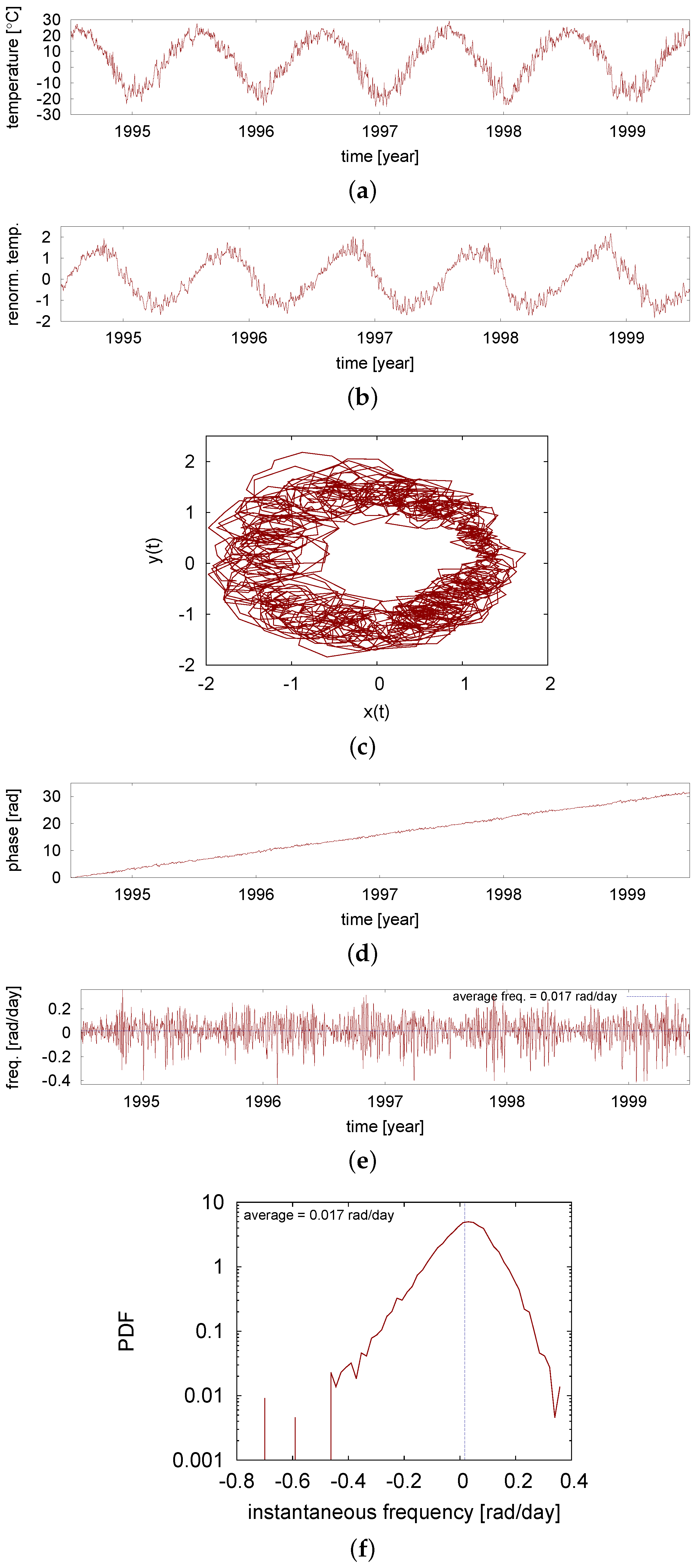
Figure 1 describes the steps taken to obtain the instantaneous frequency time series from a SAT time series. To explain the procedure, we chose a geographical region that is located in east Asia and that will be shown to have a “regular” frequency behaviour. In order to obtain trajectories that evolve around the origin, the SAT time series is first detrended and normalized to have zero mean and unit variance. We will call $x_i\left(t\right)$ this processed series. Then, we apply Hilbert transform to this series—which is considered as an oscillating signal—to obtain the complementary oscillation $y_i\left(t\right)$. We compute the Hilbert transform in the time domain by using the algorithm described in [14]. Figure 1a displays a portion of the raw SAT daily series $r_i\left(t\right)$, while the corresponding Hilbert transform $y_i\left(t\right)$ is shown in Figure 1b. By considering $x_i\left(t\right)$ and $y_i\left(t\right)$ as the coordinates of a rotating point in a plane, whose trajectory is shown in Figure 1c, we obtain the phase time series ${\phi }_i\left(t\right)$ as

$${\phi }_i\left(t\right)=\arctan \left(\frac{y_i\left(t\right)}{x_i\left(t\right)}\right).$$

Taking into account the individual signs of $x_i\left(t\right)$ and $y_i\left(t\right)$, we obtain ${\phi }_i\left(t\right)$ in the interval $[-\pi ,\pi ]$. Then, we unwrap the phase series, eliminating the jumps between the extremes of the interval to obtain the time series shown in Figure 1d. Finally, we obtain the instantaneous angular frequency series, ${\omega }_i\left(t\right)$, as the time derivative of ${\phi }_i\left(t\right)$ using a second-order discrete formula. The resulting frequency time series is shown in Figure 1e, and the probability distribution function (pdf) of frequency values is shown in Figure 1f.

Since a “regular” SAT dynamics in the extratropics consists of an annual four-season oscillation (with relatively small fluctuations due to SAT variability), in the extratropical areas, we expect an average instantaneous frequency equal to one rotation per year; that is, $2\pi /365 \mathrm{day}\approx 0.017 \mathrm{rad}/\mathrm{day}$. In fact, looking at the data presented in Figure 1e, we see that the average instantaneous frequency corresponds to the expected value. We also note the presence of negative values of the instantaneous frequency, and we remark that the pdf covers a wide range of both positive and negative frequency values (i.e., clockwise and anticlockwise rotation). We will show later that this is in part due to the fact that we are not applying any filter to the signal. While other methods can be employed to obtain an always positive frequency (see [10] for a discussion), we will show that this simple approach yields meaningful information about large-scale patterns in SAT dynamics.

We note that in a typical “regular” case (such as the one shown in Figure 1), the noisy limit cycle is well defined, since its amplitude is bigger than the irregular fluctuations; therefore, the instantaneous phase is always defined. In the next sections, we will discuss “irregular” geographical regions, where the obtained trajectories do not resemble noisy limit cycles. We will show that the “irregular” behaviours are clearly captured by Hilbert frequency analysis.

3. Results

In this section, we present the statistical analysis of the obtained time series of instantaneous frequencies: for every site, we calculate the time-averaged value of the angular frequency, ${\overline{\omega }}_i$, and its standard deviation, ${\sigma }_i$, and show with colour maps how these values are distributed over the world.

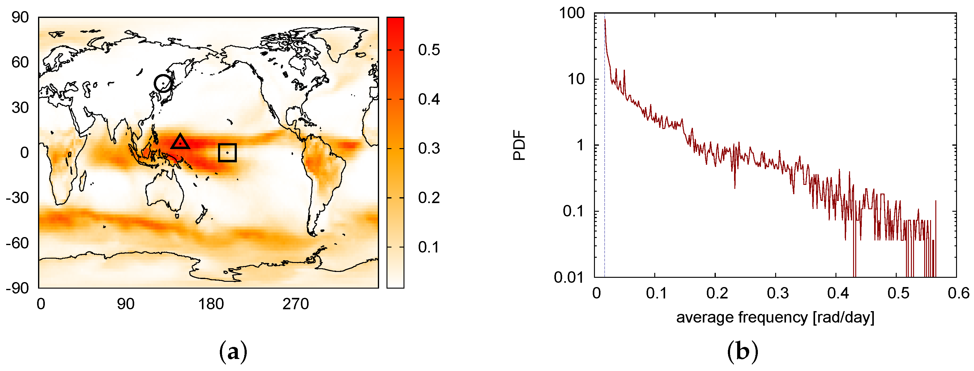
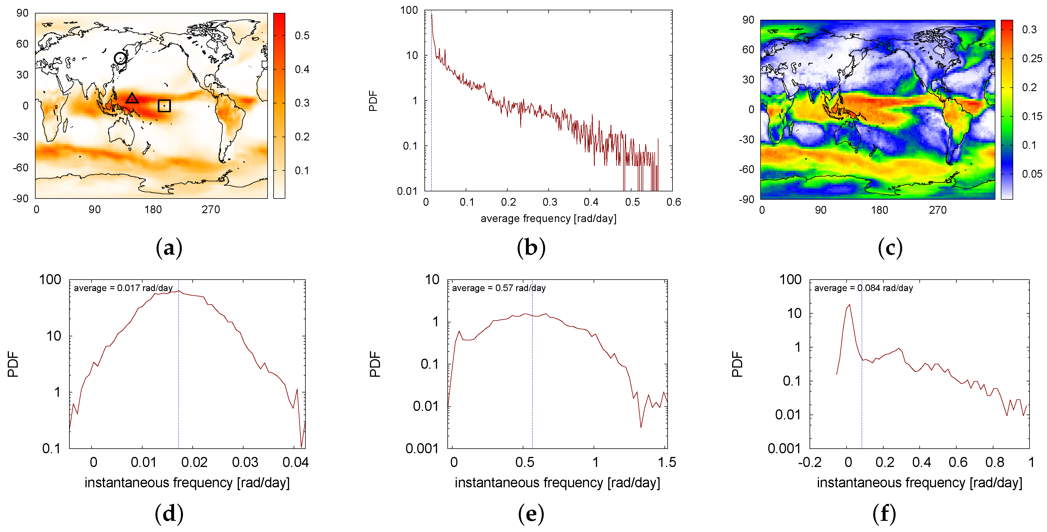
We begin by presenting the plot of the spatial distribution of time-averaged instantaneous frequency in Figure 2a. In this map, the colour code represents the averaged frequency in rad/day, and is adjusted such that white corresponds to the frequency of the annual cycle ($\approx 0.017 \mathrm{rad}/\mathrm{day}$), while red represents higher frequency values. Large-scale structures are seen, with well defined geographical regions where the average frequency is faster than that of the annual cycle. Figure 2b shows the distribution of time-averaged frequencies, weighted according to the area of each site. Next, we discuss two examples of “faster” sites.

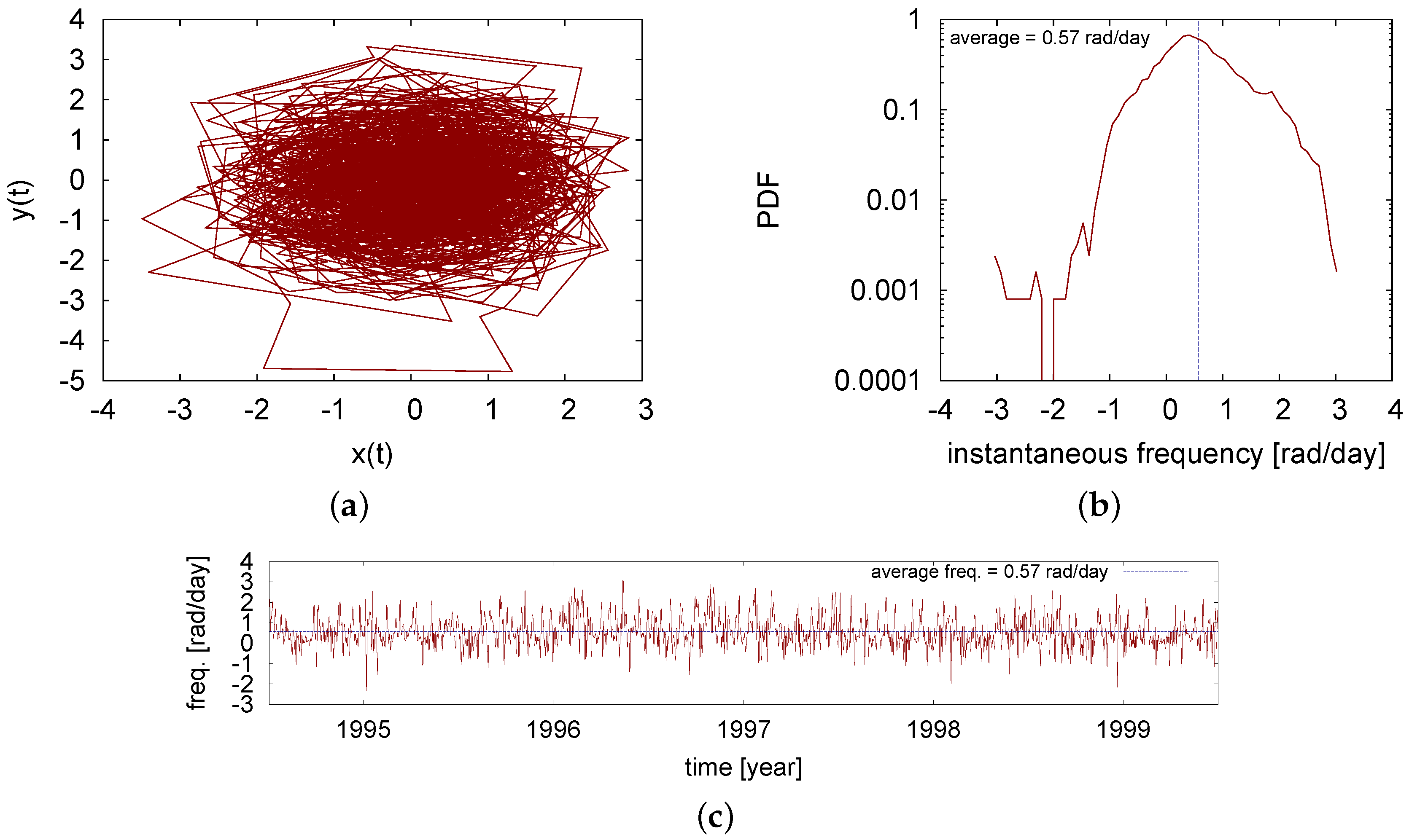
Figure 3 gives details about a site located in a red area in the Pacific Ocean (indicated in Figure 2a with a triangle): the instantaneous frequency and the corresponding trajectory are shown, during a time-interval of about 5 years. Additionally, the frequency pdf is shown, computed with all the values in the time series. A highly irregular dynamics is observed, which does not resemble a noisy limit cycle, and the fluctuations of the instantaneous frequency are larger than those in a regular site (compare the horizontal axis in Figure 1f and Figure 3b).

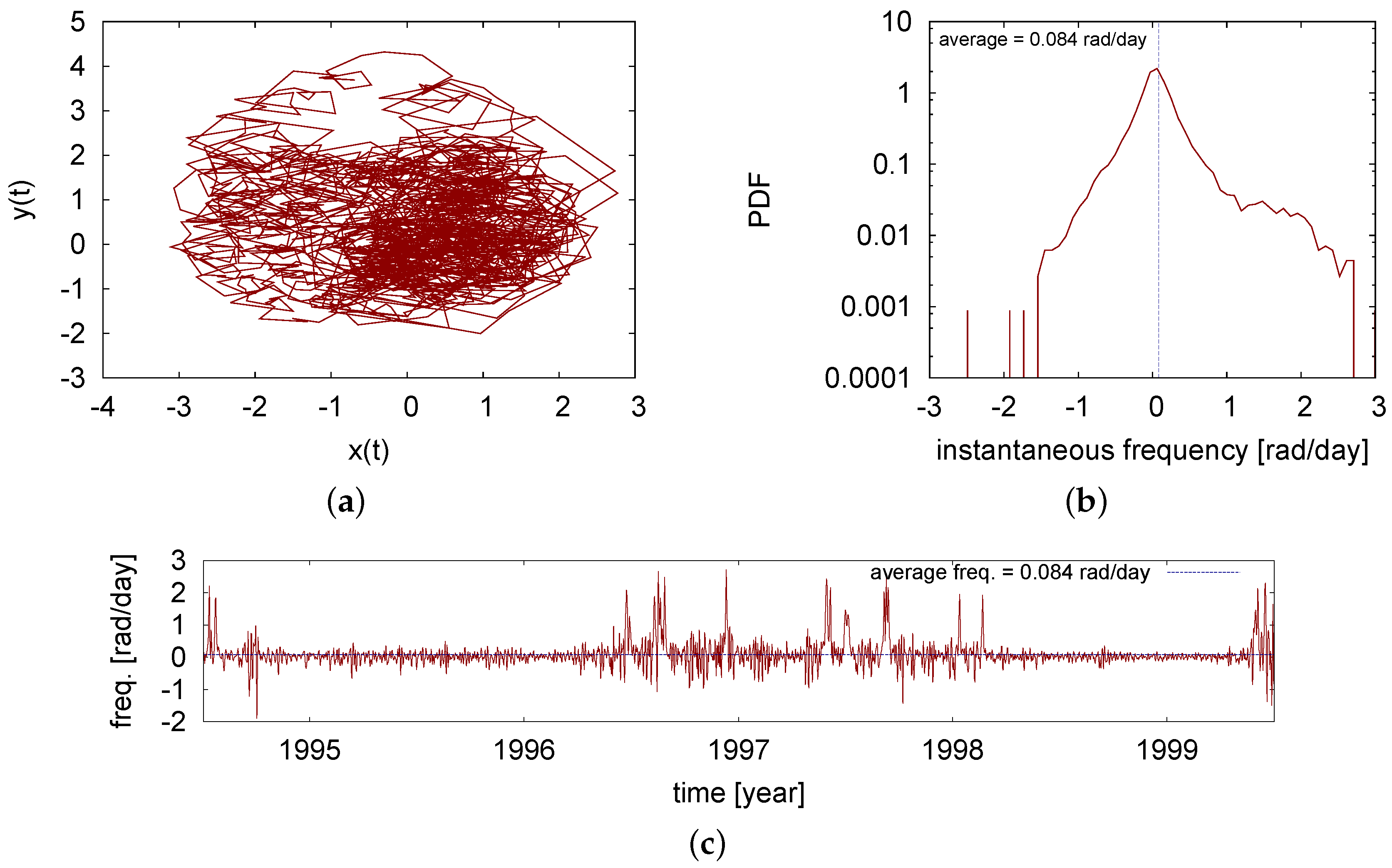
Figure 4 shows analogous results for a site located in the Pacific Ocean, in a transition area (at the border of the red area, as indicated in Figure 2a with a square). Here again we observe a highly irregular dynamics, but in contrast with the previous case, the frequency fluctuations are usually small, and only occasionally are there large fluctuations.

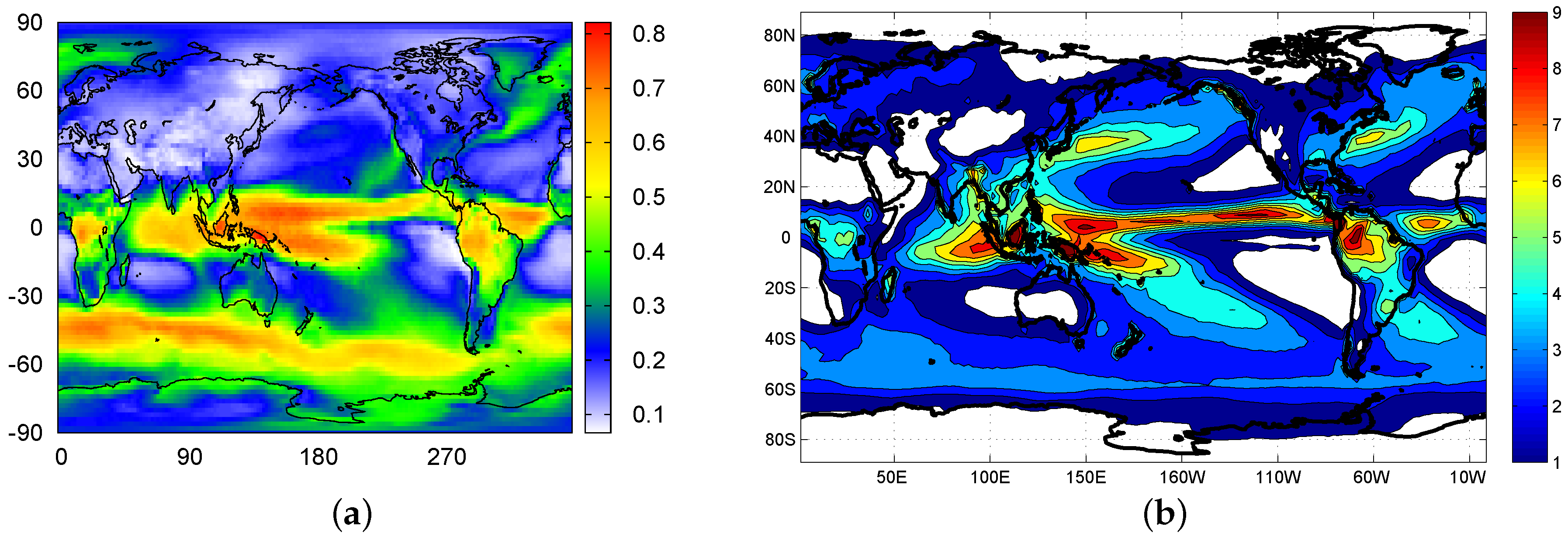
To investigate the spatial structure of frequency fluctuations, Figure 5 displays in colour code the map of the standard deviation of the frequency series (in units of rad/day) and compares it to the map of annual mean precipitation [15]. In the next section, we will discuss the similarities and differences between the two maps.

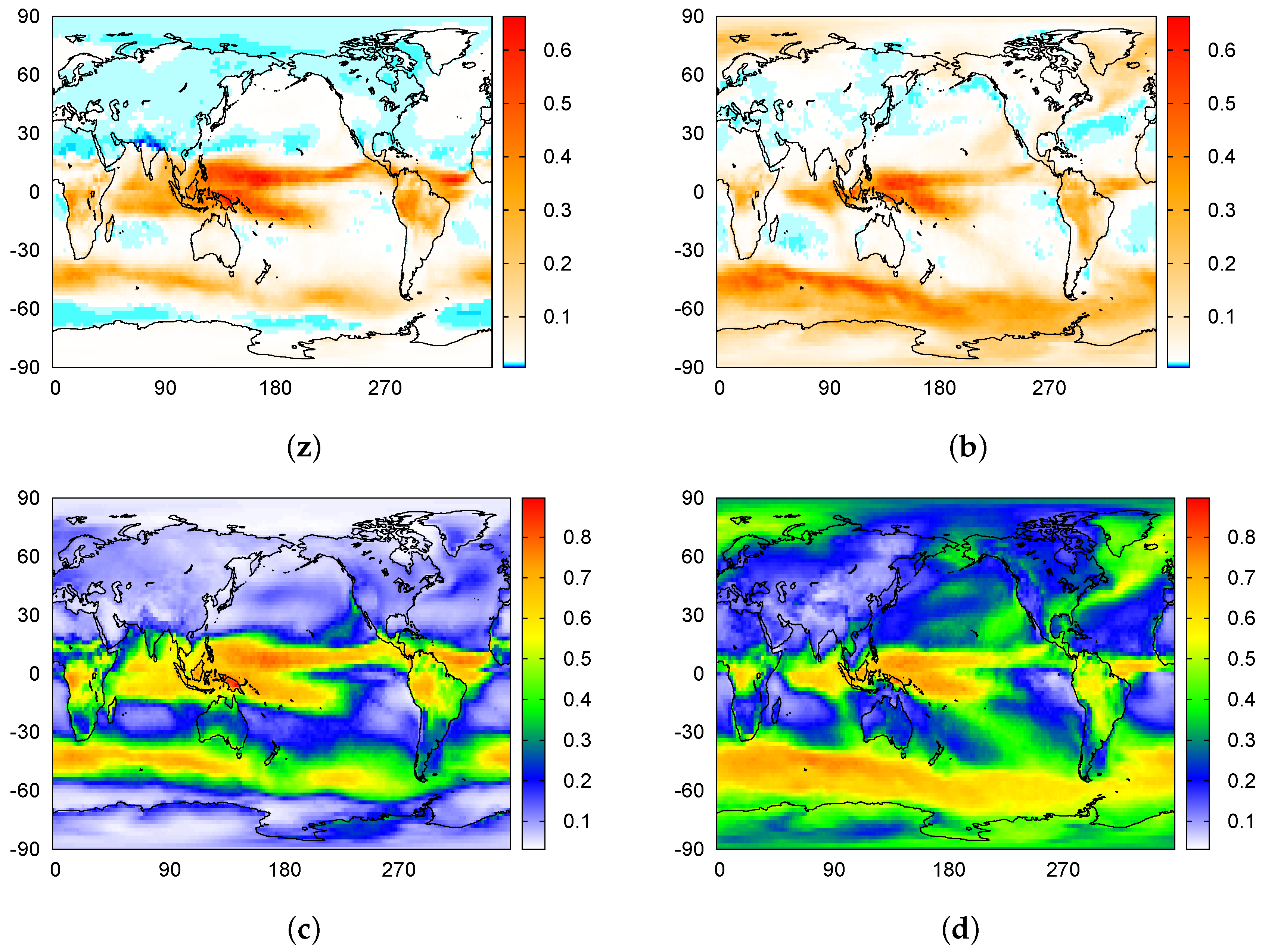
To test the robustness of our results, we calculated the instantaneous frequency in a different way: at each time, t, we compute the linear regression of the phase, ${\phi }_i\left(t\right)$, in a window of 31 days (centered in the given instant), and then we use the slope of the linear regression as the frequency at that time t. In other words, the Hilbert frequency is computed as the linear trend of the phase in a window of one month. The obtained results are presented in Figure 6: we see that the map of average frequency Figure 6a and the pdf of average frequency Figure 6b are almost identical to the ones in Figure 2. On the other hand, the map of the standard deviation, Figure 6c, is qualitatively very similar to the one in Figure 5a (it has the same spatial structures), but the standard deviation values are lower. In contrast, the distributions of instantaneous frequency change drastically: negative values are almost fully suppressed, as shown in Figure 6d–f for the same locations as before (indicated with a circle, a triangle, and a square in Figure 2a).

Lastly, in order to investigate how frequency fluctuations vary in different seasons, we extract from every frequency time-series ${\omega }_i\left(t\right)$ the values that occur during winter and the ones occurring during summer (taking into account that winter in the northern hemisphere corresponds to summer in the southern hemisphere, and vice versa). In this way, at each site we obtain two series: one of winter frequency ${\omega }_i^{\mathrm{w}}\left(t\right)$, and one of summer frequency ${\omega }_i^{\mathrm{s}}\left(t\right)$. Then, we analyze the average value and the standard deviation of the two series. The results are displayed in Figure 7. Remarkably, in the maps of average frequency, we see large regions with slower frequency dynamics (in blue) which were not previously detected (compare with Figure 2a). The maps of standard deviation show that frequency fluctuations in winter are stronger in the extratropics with respect to summer.

4. Discussion

As indicated before, the expected value of frequency—corresponding to a complete cycle in one year—is $\approx 0.017 \mathrm{rad}/\mathrm{day}$. An inspection of Figure 2a reveals that the extratropical areas tend to have this expected value (they are coloured in white). Deviations from this behaviour are characterized by a faster average frequency, and are concentrated in the tropical area and also in a southern ocean band. If we look at the distribution of Figure 2b, we can see that the most probable average frequency corresponds to that of one cycle per year (indicated with a vertical line), and we can also note that the distribution has a long tail in the higher frequency side, while it decreases sharply in the low frequency side (only very few sites have an average frequency that is slightly lower than $0.017 \mathrm{rad}/\mathrm{day}$). This lack of “slow frequency” sites can be understood as being due to solar forcing: even if the oscillation induced by solar forcing is small, it produces at least one cycle per year. In many regions, due to other climatic processes, the average frequency is higher. Thus, we detect two main types of dynamics: regular sites and faster sites. We are going to discuss them in more detail.

We begin by considering the regular sites. We have chosen a typical one to explain the calculation of instantaneous frequency in Figure 1. In addition to the annual solar cycle that produces the base of the regular trajectory, SAT dynamics has oscillations with shorter characteristic times, due to climatic processes like synoptic weather variability, which causes noisy deviations from the regular cycle. In this case, we note that the secondary oscillations have a significantly smaller amplitude than the annual cycle. If we look at the trajectory, we can see that the secondary cycles are not large enough to circle around the origin. Thus, even if they affect the instantaneous value of the frequency, they have small effect on the average value. Therefore, in this site, the trajectory describes a well defined (but noisy) limit cycle, and we refer to this geographical site as a “regular site”.

Next, we analyze geographical sites which have higher values of average frequency (examples are shown in Figure 3 and Figure 4). It is well-known that in tropical regions the annual solar cycle has a small amplitude, which is comparable to or even smaller than the amplitude of the oscillations induced by other (faster) climatological processes. Due to these additional oscillations, the Hilbert algorithm detects more than one oscillation per year, which results in the high value of frequency that we see in the red regions in Figure 2a. We note that the average frequency does not correspond to a semi-annual cycle, as could be expected due to the double crossing of the sun across the equator. We can understand the faster frequency by analyzing the noisy trajectories: the cycles produced by the faster processes dominate the trajectory and can wash out the effect of the small-amplitude solar cycle (annual or semi-annual). Since many of these fast oscillations are wide enough to circle around the origin, they are counted as complete cycles and affect the frequency, increasing its average value and creating large fluctuations.

To yield light into the climate processes that can be represented in these fluctuations, let us consider the maps shown in Figure 5: the standard deviation of frequency and the annual mean precipitation. While there are some differences in the extratropics, we observe a strong similarity between the two maps in the tropical regions. This is consistent with the fact that convective activity generates deep clouds that, on one hand, shield the surface from the solar radiation and can induce fast changes in the surface air temperature and, on the other hand, are responsible for the high level of precipitation. As for the extratropical region of high standard deviation located in the southern ocean, this region is characterized by large sea surface temperature (SST) gradients (fronts) and high eddy activity, which can strongly affect the above air temperature and can explain the strong fluctuation of instantaneous frequency.

In Figure 6 we can see the results when frequency is calculated by using the linear trend of Hilbert phase, a procedure that “washes out” the frequency fluctuations that are due to “phase noise”. The spatial patterns found in the map of time-average of frequency and in the map of standard deviation of frequency fluctuations are robust, in the sense that they are also found when the instantaneous frequency is computed with this other procedure. In contrast, the pdf of instantaneous frequency strongly depends on the procedure used to compute the frequency, and therefore we expect that—in order to extract additional information from Hilbert frequency analysis (going beyond the analysis of the mean value and of the standard deviation)—more sophisticated approaches need to be applied, such as the ones discussed in [4].

Now let us consider frequency and its fluctuations in the different seasons. Comparing the summer and winter maps shown in Figure 7, we can see that in the tropics there are no large summer–winter differences (the average value of frequency and its standard deviation tend to be the same), but in the extratropics, both the average frequency and its standard deviation tend to be larger in the winter with respect to the summer.

In the southern latitudes next to Antarctica, the average frequency is smaller (larger) than the annual cycle in summer (winter). This is likely due to the existence of sea ice during winter that isolates the atmosphere from the ocean (acting as a buffer for air–sea interaction), thus allowing faster SAT fluctuations. In the midlatitude ocean, the air–sea contrast is larger in winter than in summertime, and SST gradients are larger. Moreover, the atmosphere is more active, thus allowing faster changes in SAT fluctuations and more day-to-day variability. In the tropics, SST is high during summer, particularly off the equator, which is able to induce stronger convection leading to higher frequency in air temperature variability. Over continental areas, northern India presents the region with smallest average frequency during summer, with a value lower than the annual cycle. This is likely related to the development of the convection associated with the Indian monsoon, which induces maximum rainfall amounts over that region. However, it is unclear why convection would diminish the average frequency instead of increasing it, as is the case over the tropical oceans. Further understanding is left for future studies.

5. Conclusions

We have applied Hilbert instantaneous frequency analysis to daily SAT time series recorded over a regular grid of locations covering the Earth surface. We have found that the maps of average frequency uncover well defined large-scale patterns. In the extra-tropics, the average frequency generally corresponds to the expected one-year period of solar forcing, while the tropics generally display a faster behaviour. The results were interpreted as being due to the fact that in the tropics the amplitude of the annual oscillation is small with respect to oscillations induced by other climatological processes. Coherent structures were also found in the maps of the standard deviation of frequency fluctuations, which tend to be located over regions of strong annual precipitation. The main differences between summer and winter frequency behaviour were found in the extra-tropics, where the average frequency and the standard deviation tend to be higher during winters.

In general, the time series of instantaneous frequency displays large fluctuations (either when geographical site is a regular site with the average frequency corresponding to one cycle per year, or when geographical site is an “irregular” site that displays a faster frequency dynamics). While such large frequency fluctuations are often considered artifacts that can be removed by appropriated filtering, in the case of the SAT daily data analyzed here, the large frequency fluctuations indeed contain meaningful information about large-scale climate phenomena. Thus, our results indicate that Hilbert analysis can be a valuable tool to gain information about the dynamics of other climatological variables, and about interactions between climatological variables (e.g., SAT and SST).

A possibility of future work is to use the time series of instantaneous frequencies to construct a climate network and then compare it with the network constructed with other approaches (such as building from SAT anomalies) [16,17,18,19,20]. Additionally, it will be interesting to explore the potential of Hilbert analysis for identifying signatures of climate change in variations of the statistical properties of frequency time series.