Thermodynamics of Noncommutative Quantum Kerr Black Holes

Abstract

The thermodynamic formalism for rotating black holes, characterized by noncommutative and quantum corrections, is constructed. From a fundamental thermodynamic relation, the equations of state and thermodynamic response functions are explicitly given, and the effect of noncommutativity and quantum correction is discussed. It is shown that the well-known divergence exhibited in specific heat is not removed by any of these corrections. However, regions of thermodynamic stability are affected by noncommutativity, increasing the available states for which some thermodynamic stability conditions are satisfied.

1. Introduction

It is known that the classical thermodynamics formalism can be applied to explore the physical entropy of a black hole, using semiclassical approaches to general relativity. The best known of these approximations was proposed by Bekenstein and Hawking in order to solve the so-called information problem [1,2,3,4]. They found that the area A of the event horizon of black holes, in an asymptotically-flat spacetime, obeys a simple relation, which is the mathematical analogue of the corresponding entropy for a black hole $S_{BH}$ ($BH$, Bekenstein–Hawking). The results obtained by Bekenstein and Hawking are supported by quantum field theory in the curved spacetime formalism. This formalism is not able to give a bound for the precision with which distance measurements are made; such a bound presumably must exist, given by the Planck length. One possible way to introduce this bound is by means of the noncommutativity of spacetime. In the context of gravity, noncommutativity is usually introduced using the Seiberg–Witten map, gauging some appropriate group [5]. More recently, a new proposal to introduce an effective noncommutativity was considered, deforming the minisuperspace in cosmological models instead of the spacetime manifold, in such a way that its coordinates do not commute [6]. In this work, the latter formalism will be considered in order to take into account noncommutativity for black holes.

The thermodynamics of black holes has a long history, in particular related to the problem of thermodynamic stability. Since the seminal work of Gibbons and Hawking [7], it is known that this problem can be extended to black holes in non-asymptotically-flat spacetimes. They found that the thermodynamic information of de Sitter black holes exhibits important differences with respect to black holes on an asymptotically-flat spacetime, which was later corroborated in different works [8,9]. They found that such black holes emit radiation with a perfect blackbody spectrum. The temperature of these black holes is determined by their surface gravity, which is the same result obtained for the asymptotically-flat space case. However, in a de Sitter space, a cosmological event horizon also exists, which also emits particles with a temperature proportional to its surface gravity. Therefore, the only way that thermal equilibrium can be achieved is when both surface gravities are equal, which only occurs in a degenerate case of extreme solutions [10,11].

Regarding black holes in an AdS (Anti de Sitter) manifold, Hawking and Page [12] found that thermodynamic stability can be achieved. For this manifold, the gravitational potential produces a confinement for particles with nonzero mass, acting effectively as a cavity of finite volume, where the black hole is contained. Moreover, their heat capacity is positive, which also allows a canonical description of the system. Another motivation to study the thermodynamic stability of black holes is the known relation with the dynamical stability of those systems. For an asymptotically-flat spacetime, Schwarzschild black holes are thermodynamically unstable, but have dynamical stability [13]. On the other hand, for AdS spacetimes, it is known that thermodynamic and dynamical stability are closely related [14,15].

Since we are considering black holes in asymptotically-flat spacetime, it seems legitimate to ask if corrections like the noncommutativity or semiclassical ones are capable of modifying the thermodynamics of black holes in order to have thermodynamically-stable systems.

In [16,17,18], this is postulated to be the fundamental thermodynamic relation for black holes, which contains all thermodynamic information of the system. Under this assumption, its classical thermodynamic formalism is constructed finding that for black holes, the thermodynamic structure of the theory resembles magnetic systems instead of fluids.

As mentioned above, it is well known that for an asymptotically-flat spacetime, the temperature of black holes is proportional to its surface gravity κ, as $T=\kappa \hslash /2\pi k_{B}c$ [1]; this semiclassical result was the key that led to the Bekenstein–Hawking entropy, which is related to the area of its event horizon,

$$S_{BH}=\frac{c^3}{4G\hslash }A.$$

(1)

The appropriated metric to describe a rotating black hole is the Kerr one, which can be written as,

$$d{s}^2=-\left(1-\frac{2Mr}{\Sigma }\right)d{t}^2-\frac{4Mra{sin}^2\theta }{\Sigma }dtd\theta +\frac{\Sigma }{\Delta }d{r}^2+\Sigma d{\theta }^2+\frac{B{sin}^2\theta }{\Sigma }d{\varphi }^2;$$

(2)

where $\Sigma =r^2+a^2{cos}^2\theta$, $\Delta =r^2-2Mr+a^2$, $B={(r^2+a^2)}^2-a^2\Delta {sin}^2\theta$ and $a=J/Mc$. The area of the event horizon of a black hole is given by $A={\int }_s\sqrt{det\left|g_{\mu \nu }\right|}ds$. Applying the elements of the metric tensor given in Equation (2), the resulting area is:

$$A=8\pi G^2{M}^2{c}^{-4}\left[1+\sqrt{1-\frac{c^2{J}^2}{G^2{M}^4}}\right].$$

(3)

Substituting in Equation (1), the resulting expression is assumed to be a thermodynamic fundamental relation for Kerr black holes; with $U=M{c}^2$, the internal energy of the system and J its angular momentum. This relation can be written as [16],

$$S_{BH}(U,J)=\frac{2\pi k_B}{\hslash c}\left(\frac{G{U}^2}{c^4}+\sqrt{\frac{G^2{U}^4}{c^8}-c^2{J}^2}\right);$$

(4)

where G is the universal gravitational constant, ℏ is the reduced Planck constant, c is the speed of light in vacuum and $k_B$ is the Boltzmann constant. We are interested in the thermodynamic implications of quantum correction to Bekenstein–Hawking (BH) entropy $S_{BH}$ that have arisen in recent years, in the search for suitable candidates of quantum gravity, namely the quest for understanding microscopic states of black holes [19,20]; and the inclusion to black hole entropy of noncommutativity. This is given considering that the coordinates of minisuperspace are noncommutative [21]. Different corrections to Bekenstein–Hawking entropy have emerged from a variety of approaches in recent years, logarithmic ones are a popular choice among those; arising from quantum corrections to the string theory partition function [22]. They are related to the low energy or infrared properties of gravity and are also independent of high energy or ultraviolet properties of the theory [19,22,23,24]. In this work, the selected expression for quantum and noncommutative corrected entropy to work with, which will be denoted as $S^{★}$, is obtained according to the ideas presented in [21]. Starting from a diffeomorphism between the Kantowski–Sachs cosmological model, which describes a homogeneous, but anisotropic universe [25], and the Schwarzschild solution, whose line element inside the event horizon $r<2M$ is given by:

$$d{s}^2=-{\left(\frac{2M}{t}-1\right)}^{-1}d{t}^2+\left(\frac{2M}{t}-1\right)d{r}^2+t^2(d{\theta }^2+{sin}^2\theta d{\varphi }^2);$$

(5)

where the temporal t and the spatial r coordinates swap their role, producing a change on the causal structure of spacetime, i.e., the transformation $t\leftrightarrow r$ is performed and considering the Misner parametrization of the Kantowski–Sachs metric, it follows,

$$d{s}^2=-N^{2}d{t}^2+e^{(2\sqrt{3}\gamma )}d{r}^2+e^{(-2\sqrt{3}\gamma )}{e}^{(-2\sqrt{3}\lambda )}(d{\theta }^2+{sin}^2\theta d{\varphi }^2).$$

(6)

In this parametrization, λ and γ play the role of the Cartesian coordinates in the Kantowski–Sachs minisuperspace. Comparing Equations (5) and (6), it is straightforward to note the correspondence between the components of the metric tensor, in order to identify the functions N, γ and λ. The following step is to obtain the Wheeler–DeWitt (WDW) equation for the Kantowski–Sachs metric given in (6), whose parametrization is related with the Schwarzschild solution given in Equation (5), finding the corresponding Hamiltonian of the system H through the Arnowitt–Deser–Misner (ADM) formalism, to introduce it into the quantum wave equation $H\Psi =0$, where $\Psi (\gamma ,\lambda )$ is the wave function. This process leads to the WDW equation whose solution can be found by the separation of the variables.

We are interested in the solution that can be obtained when the symplectic structure of minisuperspace is modified, making the coordinates λ and γ obey the commutation relation $[\lambda ,\gamma ]=i\theta$, where θ is the noncommutative parameter; this relation strongly resembles noncommutative quantum mechanics. The aforementioned deformation can be introduced in terms of a Moyal product, modifying the original phase space, similarly to noncommutative quantum mechanics [26]:

$$f(\lambda ,\gamma )★g(\lambda ,\gamma )=f(\lambda ,\gamma )e^{\frac{i\theta }{2}[{\overleftarrow{\partial }}_{\lambda }{\overrightarrow{\partial }}_{\gamma }-{\overleftarrow{\partial }}_{\gamma }{\overrightarrow{\partial }}_{\lambda }]}g(\lambda ,\gamma ).$$

These modifications allow us to redefine the coordinates of minisuperspace in order to obtain a noncommutative version of the WDW equation,

$$\left[\frac{{\partial }^2}{\partial {\gamma }^2}-\frac{{\partial }^2}{\partial {\lambda }^2}+48e^{(-2\sqrt{3}\lambda +\sqrt{3}\theta P_{\gamma })}\right]\Psi (\lambda ,\gamma )=0;$$

(7)

where $P_{\gamma }$ is the momentum on coordinate γ. The above equation can be solved by the separation of the variables to obtain the corresponding wave function [6]:

$$\Psi (\lambda ,\gamma )=e^{i\sqrt{3}\nu \gamma }{K}_{i\nu }\left[4e^{(-\sqrt{3}(\lambda +\sqrt{3}\nu \theta /2))}\right];$$

(8)

where ν is the separation constant and $K_{i\nu }$ are the modified Bessel functions. It can be noticed that in Equation (8), the wave function has the form $\Psi (\lambda ,\gamma )=e^{i\sqrt{3}\nu \gamma }\Phi (\lambda )$; therefore, the dependence on the coordinate γ is the one of a plane wave. It is worth mentioning that this contribution vanishes when thermodynamic observables are calculated.

With the above wave equation for the noncommutative Kantowski–Sachs cosmological model, we are able to derive a modified noncommutative version of the entropy. For that purpose, the Feynman–Hibbs procedure is considered in order to calculate the partition function of the system [27]. In this approach, the separated differential equation for λ,

$$\left[-\frac{d^2}{d{\lambda }^2}+48e^{-2\sqrt{3}\lambda +3\nu \theta }\right]\Phi (\lambda )=3{\nu }^2\Phi (\lambda );$$

(9)

is considered, and the exponential in the potential term $V(\lambda )=48exp[-2\sqrt{3}\lambda +3\nu \theta ]$ of this equation is expanded up to second order in λ; with a change of variables, the resulting differential equation can be compared with the corresponding equation for a quantum harmonic oscillator in one dimension, which is a non-degenerate quantum system. In the Feynman–Hibbs procedure, the potential is modified by the quantum effects, which in the case of the harmonic oscillator is given by:

$$U(x)=V(\overline{x})+\frac{\beta {\hslash }^2}{24m}{V}^{″}(\overline{x});$$

where $\overline{x}$ is the mean value of x and $V^{″}(\overline{x})$ stands for the second derivative of the potential. For the considered changes of variables, the noncommutative quantum corrected potential can be written as,

$$U(x)=\frac{3}{4\pi }\frac{E_p}{l_p^2}{e}^{3\nu \theta }\left[x^2+\frac{\beta l_p^2{E}_p}{12}\right].$$

(10)

The above potential allows us to calculate the canonical partition function of the system,

$$Z(\beta )=A{\int }_{-\infty }^{\infty }{e}^{-\beta U(x)}dx;$$

(11)

where ${\beta }^{-1}$ is proportional to the Bekenstein–Hawking temperature and $A={[2\pi l_p^2{E}_p\beta ]}^{-1/2}$ is a constant. Substituting $U(x)$ into (11) and performing the integral over x, the partition function is given by:

$$Z(\beta )=\sqrt{\frac{2\pi }{3}}\frac{e^{3\nu \theta /2}}{E_p\beta }exp\left[-\frac{{\beta }^2{E}_p^2}{16\pi }{e}^{3\nu \theta }\right];$$

(12)

through this partition function, it is possible to calculate any thermodynamic observable, by means of the usual thermodynamic relations for the internal energy and the Legendre transformation for Helmholtz free energy,

$$\langle E\rangle =-\frac{\partial }{\partial \beta }lnZ(\beta );\frac{S}{k_B}=lnZ(\beta )+\beta \langle E\rangle .$$

With the equation for internal energy, it is possible to determine the value of β as a function of the Hawking temperature ${\beta }_H=8\pi M{c}^2/E_p$, obtaining:

$$\beta ={\beta }_H{e}^{-3\nu \theta }\left[1-\frac{1}{{\beta }_H{e}^{-3\nu \theta }}\frac{1}{M{c}^2}\right];$$

(13)

and with the aid of this relation and the Legendre transformation for Helmholtz free energy along with the partition function $Z(\beta )$, the entropy for the noncommutative quantum corrected black hole can be found:

$$S^{★}=S_{BH}{e}^{-3\nu \theta }-\frac{1}{2}{k}_{B}ln\left[\frac{S_{BH}}{k_B}{e}^{-3\nu \theta }\right]+\mathcal{O}(S_{BH}^{-1}{e}^{-3\nu \theta }).$$

(14)

The functional form of noncommutative quantum black hole entropy $S^{★}$ is basically the same as the quantum corrected one, besides the addition of multiplicative factor $e^{-3\nu \theta }$ to Bekenstein–Hawking entropy. For the sake of simplicity, we denote the noncommutative term in this expression as:

$$\Gamma =exp[-3\nu \theta ].$$

Through the rest of this paper, natural units $G=\hslash =k_B=c=1$ will be considered.

In this work, the previous result found for the Schwarzschild noncommutative black hole will be extended to the rotating black hole case. This extension is not straightforward, since it requires obtaining an analog expression for the noncommutative entropy of the rotating black hole, through the application of a diffeomorphism between the Kerr metric and some appropriated cosmological model, and (for instance) for the procedure presented in [21], to our knowledge, the implementation of this procedure has not been reported. However, it would be interesting to have an expression to study the effect of angular momentum on the physical properties of the system. Therefore, in order to have an approximated relation for the extended Kerr black hole entropy, the usual Bekenstein–Hawking entropy for rotating black holes, presented in Equation (4), and the generalized one found in Equation (14) will be used to obtain an entropy for rotating black holes including quantum and noncommutative effects. Starting from the fact that Equation (14) is correct, whatever be the expression for the non-approximated entropy for the quantum noncommutative Kerr black hole, it is clear that our proposed entropy will be a good approximation for small values of J when compared to the values of $U^2$. Therefore, in this approximation in the vicinity of small values of angular momentum, the coordinates of the minisuperspace, namely λ and γ, are the same as in the Schwarzschild case. Hence, the corrected entropy that we will analyze is:

$$S^{★}=2\pi \Gamma \left(U^2+\sqrt{U^4-J^2}\right)-\frac{1}{2}ln\left[2\pi \Gamma \left(U^2+\sqrt{U^4-J^2}\right)\right].$$

(15)

It is important to clarify that Equation (15) is not the only possible valid generalization for the corrected entropy of the Kerr black hole in the neighborhood of small J. We claim that this is the most natural one, since this is the natural extension from the Schwarzschild case to the rotating one. To our knowledge, there is not a general argument to claim that Equation (14) remains valid for any black hole, other than the Schwarzschild one. However, there is some evidence (not yet published) that for the case of charged black holes with quantum corrections, the functional form of Equation (14) is maintained. In the following, all of the thermodynamic expressions with super-index ★ will stand up for the noncommutative quantum corrected quantities derived from corresponding $S^{★}$ entropy, and quantities without sub-indexes or super-indexes will represent their noncommutative Bekenstein–Hawking counterparts. It is known from observational data that the noncommutative parameter in spacetime is small [28,29]; however, for entropy $S^{★}$, noncommutativity on the coordinates of minisuperspace is considered instead. It is expected that such parameter will be small, as well [30]; nonetheless, the actual bounds of θ are not well known yet.

In this work, the parameter Γ will be considered to be bounded in the interval given by $0<\Gamma \le 1$. As mentioned above, Equation (15) will be assumed as a fundamental thermodynamic relation for Kerr black holes when noncommutative and quantum corrections are considered. It is well known from classical thermodynamics that fundamental thermodynamic relations contain all thermodynamic information of the system under study [31]; as a consequence, modifications on thermodynamic information originated by the introduced corrections to entropy are carried through all thermodynamic quantities.

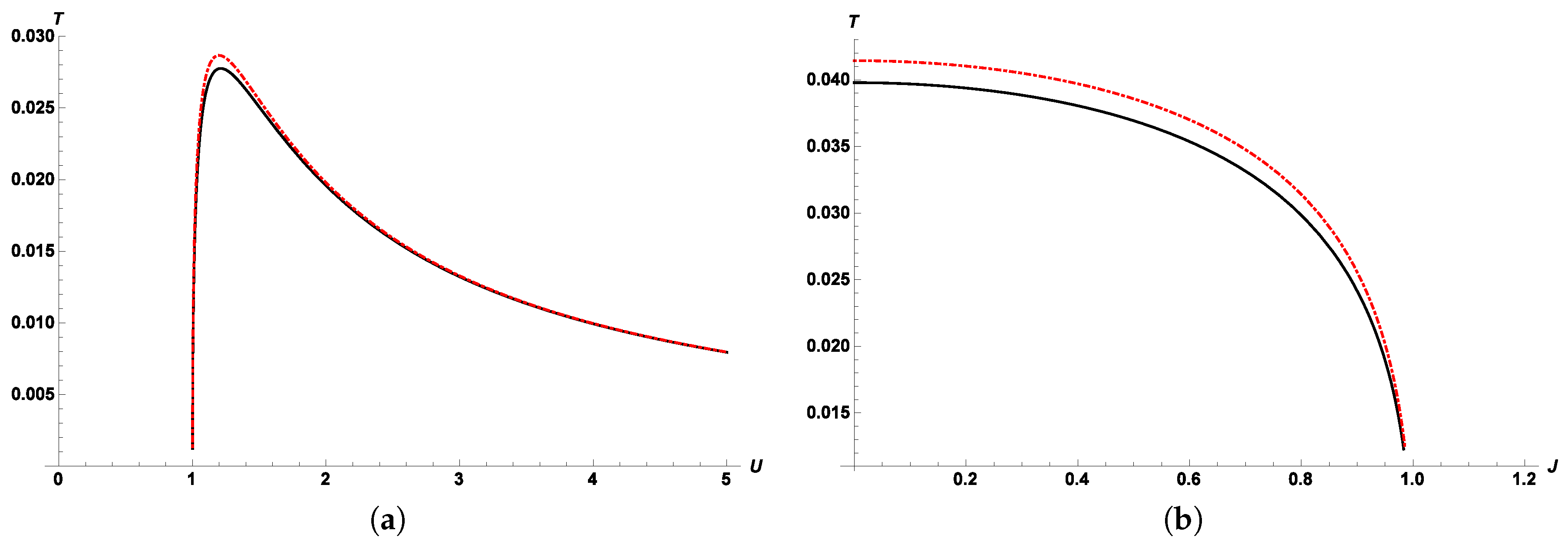
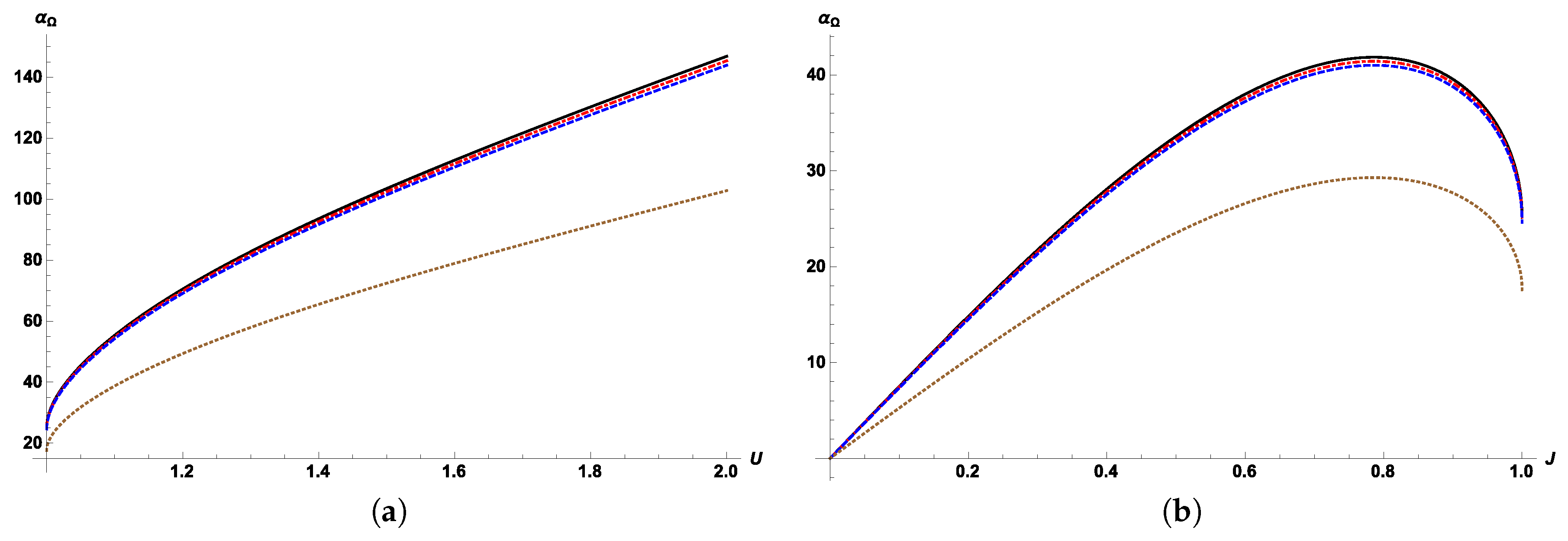
In Figure 1, curves for Bekenstein–Hawking and quantum corrected entropy are presented considering only commutative relations ($\Gamma =1$). Figure 1a considers plots for $S=S(U)$ and $S^{★}=S^{★}(U)$. Bekenstein–Hawking entropy is above the quantum correction one, including the region of small energy where entropy is thermodynamically stable [18]. Figure 1b shows the same entropy as a function of angular momentum instead, for fixed values of U; it can be noticed that Bekenstein–Hawking entropy is above $S^{★}$ in all of the considered dominion, as well. A similar analysis can be performed over noncommutativity, finding that for small values of θ, variations over S and $S^{★}$ are negligible.

The goal of this manuscript is to explore how these considerations introduced into Bekenstein–Hawking entropy change the thermodynamic information contained in this new fundamental relation, in particular thermodynamic stability and the existence of thermodynamic phase transition for these systems. In the following, an outline of this work is presented. Section 2 examines the different thermodynamic equations of state and their behavior when considering the aforementioned modifications to entropy. The same analysis is carried out in Section 3.1, considering thermodynamic response functions instead. In Section 3.2, a discussion of thermodynamic stability and phase transitions for Kerr black holes is presented. Some conclusions of this work are given in Section 4.

2. Equations of State

The fundamental Bekenstein–Hawking thermodynamic relation in entropic representation for Kerr black holes has the form $S_{BH}=S_{BH}(U,J)$. The role of thermodynamic equations of state for Kerr black holes is played by partial derivatives of entropy, $T\equiv {({\partial }_{S}U)}_J$ and $\Omega \equiv {({\partial }_{J}U)}_S$, where Ω is the angular velocity of the black hole and T is its temperature; the following relations in entropic representation are defined:

$$\frac{1}{T}\equiv {\left(\frac{\partial S_{BH}}{\partial U}\right)}_J;\frac{\Omega }{T}\equiv -{\left(\frac{\partial S_{BH}}{\partial J}\right)}_U.$$

(16)

These definitions are also valid for quantum corrected entropy $S^{★}$. Explicit equations of state in entropic representation, $T^{★}=T^{★}(U,J)$ and ${\Omega }^{★}={\Omega }^{★}(U,J)$ for noncommutative quantum corrected entropy can be written as,

$$\begin{array}{}(17\mathrm{a})& \hfill \frac{1}{T^{★}}=\frac{U\left(4\pi \Gamma \sqrt{U^4-J^2}+4\pi \Gamma U^2-1\right)}{\sqrt{U^4-J^2}};(17\mathrm{b})& \hfill \frac{{\Omega }^{★}}{T^{★}}=\frac{1}{2}\frac{J\left(4\pi \Gamma \sqrt{U^4-J^2}+4\pi \Gamma U^2-1\right)}{\sqrt{U^4-J^2}\left(U^2+\sqrt{U^4-J^2}\right)}.\end{array}$$

In addition, for noncommutative Bekenstein–Hawking entropy, the corresponding equations of state are given by,

$$\begin{array}{}(18\mathrm{a})& \hfill \frac{1}{T}=\frac{4\pi \Gamma U\left(U^2+\sqrt{U^4-J^2}\right)}{\sqrt{U^4-J^2}},(18\mathrm{b})& \hfill \frac{\Omega }{T}=\frac{2\pi \Gamma J}{\sqrt{U^4-J^2}}.\end{array}$$

The overall effect of noncommutativity over T and $T^{★}$ was analyzed, considering different values of Γ, including the commutative case ($\Gamma =1$). A noticeable effect of this parameter over these curves can be found; nonetheless, it does not change the functional behavior either of T or $T^{★}$. In order to illustrate how the introduced quantum correction affects the thermodynamic properties of black holes when compared with Bekenstein–Hawking ones, a graphical comparison between T and $T^{★}$ is performed in Figure 2 for $\Gamma =1$. As expected, Bekenstein–Hawking curves are very similar to those obtained through corrected entropy. Nevertheless, for temperature, it is possible to remark that $T^{★}(U,J)$ is slightly higher than $T(U,J)$, which is the opposite result as the one obtained for entropy, indicating that variations of entropy for a given change in its internal energy are greater for quantum corrected entropy when compared to the Bekenstein–Hawking one.

It was mentioned above that when considering values in the vicinity of $\Gamma =1$, temperature is minimally affected by noncommutativity. Smaller values of Γ were also tested; as a consequence of this consideration, maximum values capable of reaching by T and $T^{*}$ are noticeable increased. It must be remarked that changing this parameter does not alter the shape of the curves.

Regarding the angular velocity, it is an interesting result to remark that this property is independent of both quantum and noncommutative corrections to entropy, namely,

$$\Omega ={\Omega }^{★}=\frac{J}{2U\left(U^2+\sqrt{U^4-J^2}\right)}.$$

(19)

In Figure 3, angular velocity in entropic representation is presented. Figure 3a shows Ω as a function of energy for $J=1$; in this case, Ω increases until it reaches a maximum value from which it becomes complex, and it is determined by the square root that appears in the denominator of Equation (19).

3. Results and Discussion

3.1. Response Functions

Response functions contain valuable information about the thermodynamic behavior of systems; therefore, this topic must be addressed in order to study the changes, if any, introduced to black hole thermodynamic properties by noncommutativity and quantum correction to its entropy. It is possible to define thermodynamic response functions for a Kerr black hole considering Bekenstein–Hawking entropy, following the structure exhibited by magnetic systems in such a way that resulting $TdS$ equations [32] are completely analogous to their magnetic counterparts [18]. Subsequently and following this resemblance with magnetic systems, thermodynamic response functions are defined in this work without any weight factor except for heat capacities, defined with such a factor given by the inverse of temperature. Even with the above considerations, thermodynamic response functions for black holes can also be constructed following the structure commonly associated with fluids, as made in [16,33].

The first response to be analyzed is the heat capacity at constant angular momentum, defined as:

$$C_J\equiv {\left(\frac{đQ}{dT}\right)}_J=T{\left(\frac{\partial S}{\partial T}\right)}_J={\left(\frac{\partial U}{\partial T}\right)}_J;$$

(20)

in entropic representation $T=T(U,J)$, which makes it convenient to write,

$$C_J={\left(\frac{\partial T}{\partial U}\right)}_J^{-1}.$$

(21)

The corresponding heat capacity at constant angular momentum for noncommutative Bekenstein–Hawking and quantum corrected entropies is respectively given by:

$$\begin{array}{}(22\mathrm{a})& \hfill C_J=\frac{4\pi \Gamma U^2\sqrt{U^4-J^2}\left(U^2+\sqrt{U^4-J^2}\right)}{\left(U^4+J^2-2U^2\sqrt{U^4-J^2}\right)};(22\mathrm{b})& \hfill C_J^{★}=\frac{U^2\sqrt{U^4-J^2}{\left[4\pi \Gamma \sqrt{U^4-J^2}+4\pi \Gamma U^2-1\right]}^2}{\left[4\pi \Gamma U^6+U^4-12\pi \Gamma U^2{J}^2+4\pi \Gamma \sqrt{U^4-J^2}\left(U^4-J^2\right)+J^2\right]}.\end{array}$$

In Figure 4, $C_J$ is plotted as a function of internal energy for a given angular momentum in Figure 4a, and as a function of J for $U=10$ in Figure 4b. The most relevant feature exhibited in those plots is the divergence that appears in both curves, which divides heat capacity into two regions, one where $C_J$ is positive and another where specific heat becomes negative. It is well known for some time that black holes display divergences in response functions, specifically in heat capacity [16]. This feature also has been found to appear in high dimensional black hole models [33,34,35,36] and often has been related with phase transitions in black holes; this topic will be discussed and presented later.

For response functions, lower values of Γ were also tested. Specifically in Figure 4, it can be observed that varying this parameter does not change the appearance of the discontinuity of $C_J$. Although this divergence is not removed by noncommutativity, the negative part of specific heat is reduced as Γ is reduced. Divergence in $C_J$ can be traced to the roots of the denominator in Equation (22a):

$$U^4+J^2-2U^2\sqrt{U^4-J^2}=0,$$

this function has one real positive root for J,

$$J_{\text{sing}}=\sqrt{-3+2\sqrt{3}}·U^2\approx 0.68U^2.$$

(23)

which is the same value found in [16], for a Kerr black hole with Bekenstein–Hawking entropy. It must be remarked that the above root is not affected by noncommutativity corrections.

To locate this divergence across different equations of state in entropic representation, it is necessary to substitute the above value $J_{\text{sing}}$ in each equation of state. For example, for the angular velocity equation of state given in Equation (18b), if Equation (23) is substituted into this expression, it leads to:

$$\frac{\Omega }{T}\approx 5.83\Gamma ,$$

(24)

or $\Omega \approx 5.8271\Gamma T$. Therefore, in the plane Ω–T, there is a straight line that divides this plane into two regions where $C_J>0$ before the divergence and the second one where $C_J<0$. Analogously, for Bekenstein–Hawking entropy and temperature, the corresponding function that divides the S–U plane is given by the parabola determined by:

$$S\approx 10.88\Gamma U^2;$$

(25)

additionally, plane T–U is divided by the following straight line,

$$T\approx 29.73\Gamma U.$$

(26)

One highlight from Equations (24)–(26) is that all of them are linear functions of noncommutativity parameter Γ (and exponentially on θ). In Figure 5, all of the above corresponding thermodynamic planes are plotted; changes introduced by noncommutativity in each of those planes increase the area of the region where specific heat $C_J$ is positive, therefore reducing the possible values for which this response function can become negative. These changes near $\Gamma =1$ are subtle, but if Γ is taken out of this neighborhood, the area where $C_J<0$ becomes considerably smaller. This is an important result that can be related to thermodynamic stability, and it will be discussed in the next section. It is enough to indicate that noncommutativity modifies the region of available thermodynamically-stable states for the system.

Regarding the noncommutative quantum corrected specific heat capacity at constant angular momentum $C_J^{★}$, the results are fairly similar to its Bekenstein–Hawking counterpart; quantum correction does not remove the discontinuity in this response function. Similarly as $C_J$, it can be located by finding the roots in the denominator of Equation (22b),

$$4\pi \Gamma U^6+U^4-12\pi \Gamma U^2{J}^2+4\pi \Gamma U^4\sqrt{U^4-J^2}-4\pi \Gamma J^2\sqrt{U^4-J^2}+J^2=0;$$

(27)

to simplify the above expression, a set of manageable functions of J are obtained, by substituting a sequence of values for U into (27). It is possible to solve each of these function assuming $J>0$, constructing a set of coordinate pairs $(U,J)$. This process is repeated several times to obtain a relevant sample in order to accurately represent the root of Equation (27). Straightforwardly, a plot can be constructed, using the set $(U,J)$ to obtain an expression for the root by least-squares method. When plotted, points clearly exhibit a quadratic behavior, and a fitting process lead us to:

$$J_{\text{sing}}\approx 0.02176+0.68126U^2.$$

(28)

When compared to Equation (23), this result shows that discontinuity in $C_J^{★}$ is almost the same as the one found for Bekenstein–Hawking specific heat. This result is another indication, as shown above for first-order derivatives, that thermodynamic properties obtained from noncommutative quantum corrected entropy are very close to their noncommutative Bekenstein–Hawking counterparts.

Unlike the results presented in Equation (23), there is not a simple function that can be used to describe the behavior of either equation of state through its corresponding phase plane for Equation (28). The only plane that can be plotted directly is the $S^{★}$–U one, although its functional behavior is not simple. Correspondingly to $C_J$, the exhibited behavior in this plane for quantum corrected expression is very similar to the one obtained for the noncommutative Bekenstein–Hawking one, in Figure 5b; including the role played by parameter Γ. If $C_J$ and $C_J^{★}$ are compared in the commutative case, it is found that $C_J(U,J)>C_J^{★}(U,J)$ by a slight margin in all of their dominion. Another response function that can be defined for Kerr black holes is the isothermic rotational susceptibility [18],

$${\chi }_T\equiv {\left(\frac{\partial J}{\partial \Omega }\right)}_T.$$

(29)

Alternative functional forms for this response function can be obtained in entropic representation. With some algebraic manipulation, it is possible to write isothermic rotational susceptibility as:

$${\chi }_T={\left[{\left(\frac{\partial \Omega }{\partial J}\right)}_U-\frac{{(\partial \Omega /\partial U)}_J}{{(\partial T/\partial U)}_J}{\left(\frac{\partial T}{\partial J}\right)}_U\right]}^{-1};$$

(30)

it is possible to work in entropic representation with the above result since both equations of state $T=T(U,J)$ and $\Omega =\Omega (U,J)$ are available.

For noncommutative Bekenstein–Hawking entropy, isothermic rotational susceptibility can be written as:

$${\chi }_T=-\frac{2}{U^3}\left[\left(U^2+\sqrt{U^4-J^2}\right)\left(U^4+J^2-2U^2\sqrt{U^4-J^2}\right)\right];$$

(31)

a remarkable feature of this material property is that it is independent of the noncommutative parameter Γ, in analogy with the angular velocity presented in Equation (19). Furthermore, ${\chi }_T$ is well defined in all of its domain, opposite to $C_J$. Plots for ${\chi }_T$ are presented in Figure 6; from these curves, it can be noted that ${\chi }_T\to 0$ when $J\approx 0.68U^2$ or equivalently, $U\approx 1.21\sqrt{J}$. ${\chi }_T(U)$ has a region of negative values, which is also related to thermodynamic stability.

With respect to noncommutative quantum corrected entropy, its corresponding isothermal rotational susceptibility is obtained by the application of Equation (30),

$${\chi }_T^{★}={\displaystyle \frac{-4\pi \Gamma U^6-U^4+12\pi \Gamma U^2{J}^2-J^2-4\pi \Gamma {(U^4-J^2)}^{3/2}}{-8\pi \Gamma U^8-U^6+4\pi \Gamma U^4{J}^2+2U^2{J}^2+\sqrt{U^4-J^2}(-8\pi \Gamma U^6-U^4+J^2)}}\times 2U{\left(U^2+\sqrt{U^4-J^2}\right)}^2;$$

(32)

this relation is indeed a function of Γ, and it is presented in Figure 6. The effect of noncommutativity in ${\chi }_T^{★}$ is almost nonexistent, and if different values of this parameter near $\Gamma =1$ are plotted together for ${\chi }_T^{★}$, all resulting curves overlap. Only when the vicinity near $\Gamma \to 0$ is considered, the noncommutativity effect on ${\chi }_T^{★}$ is perceivable. Changes produced by Γ in the numerator of Equation (32) are countered by its role in the denominator of the same expression.

${\chi }_T^{★}$ goes to zero around $J\approx 0.7$ for $U=1$, which corresponds to the location of divergence for $C_J^{★}$. The negative region still appears in ${\chi }_T^{★}$ as observed in Bekenstein–Hawking isothermal rotational susceptibility. Additionally, if both ${\chi }_T$ and ${\chi }_T^{★}$ are compared, the latter is always slightly above the former, namely ${\chi }_T(U,J)<{\chi }_T^{★}(U,J)$. Another thermodynamic response function to be analyzed is the isentropic rotational, defined as [18]:

$${\chi }_S\equiv {\left(\frac{\partial J}{\partial \Omega }\right)}_S;$$

(33)

similarly to ${\chi }_T$, it is straightforward to obtain by rewriting in terms of U and J,

$${\chi }_S={\left[{\left(\frac{\partial \Omega }{\partial J}\right)}_U+\Omega {\left(\frac{\partial \Omega }{\partial U}\right)}_J\right]}^{-1}.$$

(34)

This relation leads to the same result for both noncommutative Bekenstein–Hawking and quantum corrected entropies since $\Omega ={\Omega }^{★}$, as shown in Equation (19). Therefore,

$${\chi }_S={\chi }_S^{★}=4U^3;$$

(35)

which is well defined in all of its dominion. The independence of Γ in the above result is a consequence that for both S and $S^{★}$, angular velocity is also independent of this parameter.

For Kerr black holes, specific heat can also be defined maintaining constant angular velocity,

$$C_{\Omega }\equiv {\left(\frac{đQ}{dT}\right)}_{\Omega }=T{\left(\frac{\partial S}{\partial T}\right)}_{\Omega };$$

(36)

$TdS$ equations provide a set of algebraic relations between response functions that can be applied in order to find analytical expressions for $C_{\Omega }$ and $C_{\Omega }^{★}$. The following relations between material properties arise [18]:

$$\begin{array}{}(37\mathrm{a})& \hfill {\chi }_T(C_{\Omega }-C_J)=T{\alpha }_{\Omega }^2;(37\mathrm{b})& \hfill C_{\Omega }({\chi }_T-{\chi }_S)=T{\alpha }_{\Omega }^2;(37\mathrm{c})& \hfill {\chi }_S{C}_{\Omega }={\chi }_T{C}_J.\end{array}$$

where ${\alpha }_{\Omega }$ is the coefficient of thermally-induced rotation. Heat capacity at constant angular velocity can be obtained directly from Equation (37c).

Therefore, specific heat for noncommutative Bekenstein–Hawking entropy is given by:

$$C_{\Omega }=\frac{2\pi \Gamma \sqrt{U^4-J^2}}{U^4}\left(-2U^2\sqrt{U^4-J^2}-2U^4+J^2\right);$$

(38)

this expression is well defined in all of the domain of its variables and has one discontinuity in the trivial case where $U=0$ (or $M=0$). In Figure 7, this response function is presented for different values of Γ; it can be noticed that $C_{\Omega }$ is negative in all of its domain. Noncommutativity reduces the negativity of this heat capacity, finding $C_{\Omega }\to 0$ as $\Gamma \to 0$. Nevertheless, this response function remains always negative.

Considering noncommutative quantum corrected entropy, specific heat capacity at constant angular velocity can be expressed as:

$$C_{\Omega }^{★}=-\frac{1}{2}\frac{\sqrt{U^4-J^2}{(4\pi \Gamma U^2+4\pi \Gamma \sqrt{U^4-J^2}-1)}^2(-2U^4-2U^2\sqrt{U^4-J^2}+J^2)}{-8\pi \Gamma U^8-U^6+4\pi \Gamma U^4{J}^2+2U^2{J}^2-(8\pi \Gamma U^6+U^4-J^2)\sqrt{U^4-J^2}};$$

(39)

its graphical representation is very similar to the one exhibited by $C_{\Omega }$. Although parameter Γ plays a more complicated role in Equation (37), the overall effect of noncommutativity in $C_{\Omega }^{★}$ leads to a very close behavior to the one observed in $C_{\Omega }$. A direct comparison between both response functions shows that $C_{\Omega }^{★}(U,J)>C_{\Omega }(U,J)$ in all of their domain.

The last response function of Kerr black holes studied in this work is the coefficient of thermally-induced rotation ${\alpha }_{\Omega }$ [18],

$${\alpha }_{\Omega }\equiv {\left(\frac{\partial J}{\partial T}\right)}_{\Omega }.$$

(40)

This material property is also calculated indirectly via relations between response functions, either Equation (37a) or Equation (37b). For noncommutative Bekenstein–Hawking entropy,

$${\alpha }_{\Omega }=\frac{4\pi \Gamma J}{U^3}\left(U^2+\sqrt{U^4-J^2}\right)\sqrt{5U^4+4U^2\sqrt{U^4-J^2}-J^2};$$

(41)

it can be remarked that ${\alpha }_{\Omega }$ is well behaved and has no discontinuities, excluding $U=0$. This function is presented in Figure 8. It can be noticed that ${\alpha }_{\Omega }$ is reduced when smaller values of Γ are considered.

Noncommutative quantum corrected coefficient ${\alpha }_{\Omega }^{★}$ is given by,

$$\begin{array}{c}{\alpha }_{\Omega }^{★}={\displaystyle \frac{UJ\left(U^2+\sqrt{U^4-J^2}\right){\left(4\pi \Gamma U^2+4\pi \Gamma \sqrt{U^4-J^2}-1\right)}^{3/2}}{-8\pi \Gamma U^8-U^6+4\pi \Gamma U^4{J}^2+2U^2{J}^2+\sqrt{U^4-J^2}(-8\pi \Gamma U^6-U^4+J^2)}}\\ \times {\left[36\pi \Gamma U^6-5U^4-20\pi \Gamma U^2{J}^2+J^2-\sqrt{U^4-J^2}(-36\pi U^4+4\pi J^2+4U^2)\right]}^{1/2}.\end{array}$$

(42)

Analogously to other response functions, quantum corrected coefficient ${\alpha }_{\Omega }^{★}$ has almost the same behavior as its Bekenstein–Hawking counterpart. If both curves are plotted together, it is found that ${\alpha }_{\Omega }(U,J)>{\alpha }_{\Omega }^{★}(U,J)$. As a summary, a comparison of thermodynamic properties between noncommutative Bekenstein–Hawking and quantum corrected entropies is presented in

Table 1. Comparison between thermodynamic properties of noncommutative Bekenstein–Hawking and noncommutative quantum corrected entropies.

Response Functions	Equations of State	Fundamental Relation
$C_J>C_J^{★}$	$T<T^{★}$	$S>S^{★}$
${\chi }_T<{\chi }_T^{★}$	$\Omega ={\Omega }^{★}$	-
${\chi }_S={\chi }_S^{★}$	-	-
$C_{\Omega }<C_{\Omega }^{★}$	-	-
${\alpha }_{\Omega }>{\alpha }_{\Omega }^{★}$	-	-

.

In the following subsection, information provided by response functions will be used to determine whether Kerr black holes are thermodynamically stable or not.

3.2. Thermodynamic Stability and Phase Transition

From the analysis performed on thermodynamic response functions for both, noncommutative S and $S^{★}$, an interesting result arises: specific heat capacity at constant angular momentum exhibits a singularity as shown in Equations (23) and (28). Discontinuity in $C_J$ for Bekenstein–Hawking entropy has been known for some time [8,16], and it is associated with a second-order (or continuous) phase transition. Expressions calculated from Bekenstein–Hawking entropy are more manageable, and for the sake of simplicity, the following analysis is performed considering only the Bekenstein–Hawking thermodynamic properties. It is expected that results obtained with these considerations are prominently similar to the ones expected for quantum corrected properties.

Thermodynamic systems passing through a first-order phase transition have physical states for which parts of the system are in different phases, or a phase coexistence, constituting a series of non-homogeneous states appearing below the critical point, where phase boundaries vanish. Often, these states can be identified with the aid of thermodynamic diagrams, as P–V diagrams for fluids. During the phase transition, the equation of state remains constant; therefore, a mechanical and thermal equilibrium exists [37,38]. Maxwell construction is a correction to violation in the van der Waals equation of the requirement to have a constant pressure with volume in isotherms of the phase diagram during a first-order phase transition [39]. It is helpful to find the critical point of a system in a first-order phase transition, if it exists.

For Kerr black holes, isotherms in the Ω–J plane must be analyzed. Criteria to find the critical point are based on the pair of conjugate variables, angular velocity and angular momentum, for which the following requirements must be satisfied:

$${\left(\frac{\partial \Omega }{\partial J}\right)}_{T_C}=0,{\left(\frac{{\partial }^2\Omega }{\partial J^2}\right)}_{T_C}=0;$$

(43)

recalling Equation (29), it implies that isothermic rotational susceptibility must be singular at this critical point ${\chi }_T\to \infty$. As shown, ${\chi }_T$ does not have any divergence and is well behaved. Therefore, there is no critical point for Kerr black holes. More evidence of this result can be found when constructing the isotherms in the phase diagram in the plane Ω–J. Changes in the concavity of the curves are expected if the system passes through a first-order phase transition; this is the region of inhomogeneous states, and it is commonly named the van der Waals loop, since this was first observed for the van der Waals equation.

In order to construct the corresponding isotherm for noncommutative Bekenstein–Hawking–Kerr black holes $\Omega =\Omega (J,T)$, it is easier to proceed from the thermodynamic fundamental relation in energy representation $U(S,J)$ [18],

$$U=\frac{1}{2}\sqrt{\frac{S}{\pi \Gamma }+\frac{4\pi \Gamma J^2}{S}},\Omega =\frac{2{\pi }^{3/2}\Gamma J}{S\sqrt{\frac{S^2+4{\pi }^2{\Gamma }^2{J}^2}{\Gamma S}}};$$

(44)

using Equation (18a) for temperature, it is straightforward to obtain:

$$J={\left(4{\Omega }^2\left\{{\left[{\left(\frac{2\pi \Gamma T}{\Omega }\right)}^2+1\right]}^{3/4}+\left(\frac{2\pi \Gamma T}{\Omega }\right){\left[{\left(\frac{2\pi \Gamma T}{\Omega }\right)}^2+1\right]}^{1/4}\right\}\right)}^{-1}.$$

(45)

Inverse function $\Omega (T,J)$ can be estimated, and it is presented in Figure 9 for different isotherms, showing the commutative case. It was not possible to find an analytical expression for this relation. As noticed in this figure, for a given value of J, there are two corresponding values of Ω, which can be interpreted as two possible cases for Kerr black holes, one of small mass and another with a larger one. When small temperatures are considered, it can be noticed that angular momentum has greater values available. There is no evidence of changes in the concavity of the isotherms in plane Ω–J, which implies that there is no van der Waals loop. The last piece of evidence is that the analogy of the Maxwell construction for noncommutative Kerr black holes is attempted to be performed; this procedure is not satisfied by any value in their domain, indicating once again that there is no critical point. Therefore, the continuity of first derivatives along with the lack of a critical point indicate that Kerr black holes do not pass through a first-order phase transition.

Negative values exhibited by material properties are directly linked with the thermodynamic stability of the system. Thermodynamic equilibrium states are characterized by an extremal principle, either maximal entropy or, equivalently, a minimum in any other thermodynamic potential. In order to ensure that those potentials are stable, they must be concave functions of their natural variables. In particular, for Kerr black holes, Gibbs potential $G(T,\Omega )$ and Helmholtz free energy $F(T,J)$ must be concave functions of both temperature and angular velocity, temperature and angular momentum, respectively. Using Legendre transformations for Kerr black holes [18],

$$S=-{\left(\frac{\partial G}{\partial T}\right)}_{\Omega }=-{\left(\frac{\partial F}{\partial T}\right)}_J;$$

concavity criteria require that second derivatives satisfy the following relations [32,39]:

$${\left(\frac{{\partial }^{2}F}{\partial T^2}\right)}_J=-{\left(\frac{\partial S}{\partial T}\right)}_J=-\frac{1}{T}{C}_J\le 0(\text{For}:\Delta U\to 0),$$

(46)

$${\left(\frac{{\partial }^{2}G}{\partial {\Omega }^2}\right)}_T=-{\left(\frac{\partial J}{\partial \Omega }\right)}_T=-{\chi }_T\le 0(\text{For}:\Delta J\to 0),$$

(47)

$${\left(\frac{{\partial }^{2}G}{\partial T^2}\right)}_{\Omega }=-{\left(\frac{\partial S}{\partial T}\right)}_{\Omega }=-\frac{1}{T}{C}_{\Omega }\le 0(\text{For}:\Delta U\to 0,\Delta J\to 0).$$

(48)

From the above relations and results found in Section 3.1, particularly Equations (22), (31) and (38), it is evident that Kerr black holes have regions where thermodynamic states do not meet these requirements, since $C_J$, ${\chi }_T$ and $C_{\Omega }$ are negative in those regions.

Geometric interpretation in the three-dimensional thermodynamic space S–U–J of Equations (46)–(48) can be found in the corresponding figures of each response function (see Figure 4, Figure 6 and Figure 7, respectively). For variations in internal energy, the change of sign in $C_J$ implies that noncommutative quantum corrected Kerr black holes are in weakly stable states (where some of the stability conditions are fulfilled, which are also known as metastable states), for low masses, becoming unstable at greater ones, as noticed in Figure 4a. For variations in angular momentum alone, as shown in Figure 6, isothermic rotational susceptibility becomes negative in the region above $J=0.68U^2$, namely greater values of J; the system is also in weakly stable states for low values of J. When variations in both U and J are considered, noncommutative quantum corrected Kerr black holes are always unstable, since $C_{\Omega }\le 0$ in all of its dominion, as presented in Figure 7.

Although the thermodynamic stability of extended Kerr black holes is not modified, varying the value of Γ has a direct consequence on accessible weakly stable states, for example increasing the region where $C_J$ is positive. As shown in Figure 5, smaller values of the noncommutativity parameter force the system to exist in a larger set of metastable states.

The existence of thermodynamic instability and the divergence in $C_J$ reveal that the system goes through a series of metastable states, from a low mass black hole to a higher mass one, in analogy with other metastable phenomena, such as superheating or supercooling. Nevertheless, the lack of a microscopic description for black holes makes it not possible to be sure that Kerr black holes pass through a continuous phase transition [40]. However, the violation of stability criteria is a strong thermodynamic argument to support this hypothesis [31].

4. Conclusions

An analysis on the thermodynamic properties of noncommutative quantum corrected Kerr black holes using an approximate relation was presented. Although the resulting expressions are mathematically more complicated, the thermodynamic properties still retain the same functional behavior with respect to those calculated via Bekenstein–Hawking entropy. It was explicitly proven that Kerr black holes do not pass through a first-order phase transition; since the local criteria to find the critical point is not fulfilled for any value in the domain, corresponding isotherms do not exhibit van der Waals loops, and the Maxwell construction cannot be obtained; all of which are characteristic of this kind of transition. Nonetheless, some second derivatives exhibit a change of sign, which is an indication that those states are thermodynamically unstable. This instability and the nonexistence of a critical point suggest that the system goes through metastable states, from a low mass black hole to a high mass one, in a continuous phase transition. Regarding the effective noncommutativity incorporated in the coordinates of minisuperspace, outside the vicinity where $\Gamma \approx 1$, changes introduced by this parameter over the thermodynamic information of the system are relevant. In particular, it has an impact on the stability of Kerr black holes, allowing the system to be thermodynamically metastable for a wider set of states. Despite only an approximated expression being considered, it allowed us to study the effect of angular momentum for quantum noncommutative black holes. It would be interesting to have a complete description for noncommutative rotating black holes, in order to be compared with the results presented in this work, in particular those related with thermodynamic stability.

References

1. Hawking, S.W. Gravitational Radiation from Colliding Black Holes. Phys. Rev. Lett. 1971, 26, 1344–1346. [Google Scholar] [CrossRef]
2. Hawking, S.W. Black holes and thermodynamics. Phys. Rev. D 1976, 13. [Google Scholar] [CrossRef]
3. Bekenstein, J.D. Black Holes and Entropy. Phys. Rev. D 1973, 7. [Google Scholar] [CrossRef]
4. Bekenstein, J.D. Generalized second law of thermodynamics in black-hole physics. Phys. Rev. D 1974, 9. [Google Scholar] [CrossRef]
5. Chamseddine, A.H. Deforming Einstein’s gravity. Phys. Lett. B 2001, 504, 33–37. [Google Scholar] [CrossRef]
6. García-Compeán, H.; Obregón, O.; Ramírez, C. Noncommutative Quantum Cosmology. Phys. Rev. Lett. 2002, 88, 161301. [Google Scholar] [CrossRef] [PubMed]
7. Gibbons, G.W.; Hawking, S.W. Cosmological event horizons, thermodynamics, and particle creation. Phys. Rev. D 1977, 15, 2738–2751. [Google Scholar] [CrossRef]
8. Davies, P.C.W. Thermodynamic phase transitions of Kerr-Newman black holes in de Sitter space. Class. Quantum Gravity 1989, 6. [Google Scholar] [CrossRef]
9. Chamblin, A.; Emparan, R.; Johnson, C.V.; Myers, R.C. Charged AdS black holes and catastrophic holography. Phys. Rev. D 1999, 60, 064018. [Google Scholar] [CrossRef] [Green Version]
10. Nariai, H. On some static solutions of Einstein’s gravitational field equations in a spherically symmetric case. Sci. Rep. Tohoku Univ. 1950, 34, 160–167. (In Japanese) [Google Scholar]
11. Nariai, H. On a new cosmological solution of Einstein’s field equations of gravitation. Sci. Rep. Tohoku Univ. 1950, 35, 62–67. (In Japanese) [Google Scholar]
12. Hawking, S.W.; Page, D.N. Thermodynamics of black holes in anti-de Sitter space. Commun. Math. Phys. 1983, 87, 577–588. [Google Scholar] [CrossRef]
13. Price, R.H. Nonspherical Perturbations of Relativistic Gravitational Collapse. I. Scalar and Gravitational Perturbations. Phys. Rev. D 1972, 5. [Google Scholar] [CrossRef]
14. Gubser, S.S.; Mitra, I. The evolution of unstable black holes in anti-de Sitter space. J. High Energy Phys. 2001, 108. [Google Scholar] [CrossRef]
15. Hollands, S.; Wald, R.M. Stability of Black Holes and Black Branes. Commun. Math. Phys. 2013, 321, 629–680. [Google Scholar] [CrossRef]
16. Davies, P.C.W. The thermodynamics of black holes. Proc. R. Soc. Lond. A 1977, 353, 499–521. [Google Scholar] [CrossRef]
17. Martinez, E.A. The postulates of gravitational thermodynamics. Phys. Rev. D 1996, 54. [Google Scholar] [CrossRef]
18. Escamilla, L.; Torres-Arenas, J. Thermodynamic response functions and Maxwell relations for a Kerr black hole. Rev. Mex. Fis. 2014, 60, 59–68. [Google Scholar]
19. Keeler, C.; Larsen, F.; Lisbão, P. Logarithmic corrections to 𝒩 ≥ 2 black hole entropy. Phys. Rev. D 2014, 90, 043011. [Google Scholar] [CrossRef]
20. Sen, A. Logarithmic corrections to Schwarzschild and other non-extremal black hole entropy in different dimensions. J. High Energy Phys. 2013, 4, 156. [Google Scholar] [CrossRef]
21. López-Domínguez, J.C.; Obregón, O.; Sabido, M.; Ramírez, C. Towards Noncommutative Quantum Black Holes. Phys. Rev. D 2006, 74, 084024. [Google Scholar] [CrossRef]
22. Sen, A. Logarithmic corrections to 𝒩 ≥ 2 black hole entropy: An infrared window into the microstates. Gen. Relativ. Gravit. 2012, 44, 1207–1266. [Google Scholar] [CrossRef]
23. Banerjee, S.; Gupta, R.K.; Mandal, I.; Sen, A. Logarithmic corrections to and black hole entropy: A one loop test of quantum gravity. J. High Energy Phys. 2011, 3, 143. [Google Scholar] [CrossRef]
24. Carlip, S. Logarithmic corrections to black hole entropy, from the Cardy formula. Class. Quantum Gravity 2000, 17. [Google Scholar] [CrossRef]
25. Kantowski, R.; Sachs, R.K. Some Spatially Homogeneous Anisotropic Relativistic Cosmological Models. J. Math. Phys. 1966, 7. [Google Scholar] [CrossRef]
26. Gamboa, J.; Loewe, M.; Rojas, J.C. Noncommutative quantum mechanics. Phys. Rev. D 2011, 64, 067901. [Google Scholar] [CrossRef]
27. Feynman, R.P.; Hibbs, A.R. Quantum Mechanics and Path Integrals, 1st ed.; McGraw-Hill: New York, NY, USA, 1965. [Google Scholar]
28. Aoki, H.; Ishibashi, N.; Iso, S.; Kawai, H.; Kitazawa, Y.; Tada, T. Noncommutative Yang-Mills in IIB Matrix Model. Nucl. Phys. B 2000, 565, 176–192. [Google Scholar] [CrossRef]
29. Joby, P.K.; Chingangbam, P.; Das, S. Constraint on noncommutative spacetime from PLANCK data. Phys. Rev. D 2015, 91, 083503. [Google Scholar]
30. Guzmán, W.; Sabido, M.; Socorro, J. On noncommutative minisuperspace and the Friedmann equations. Phys. Lett. B 2011, 697, 271–274. [Google Scholar] [CrossRef]
31. Callen, H.B. Thermodynamics and an Introduction to Thermo-Statistics, 2nd ed.; John Willey & Sons: Hoboken, NJ, USA, 1985; pp. 35, 183 and 215. [Google Scholar]
32. Stanley, H.E. Introduction to Phase Transitions and Critical Phenomena, 1st ed.; Oxford University Press: London, UK, 1971; pp. 29–34. [Google Scholar]
33. Poshteh, M.B.J.; Mirza, B.; Sherkatghanad, Z. Phase transition, critical behavior, and critical exponents of Myers-Perry black hole. Phys. Rev. D 2013, 88, 024005. [Google Scholar] [CrossRef]
34. Banerjee, R.; Roychowdhury, D. Thermodynamics of phase transition in higher dimensional AdS black holes. J. High Energy Phys. 2011, 1111, 004. [Google Scholar] [CrossRef]
35. Mansoori, S.A.H.; Mirza, B. Correspondence of phase transition points and singularities of thermodynamic geometry of black holes. Eur. Phys. J. C 2014, 74, 2681. [Google Scholar] [CrossRef]
36. Lala, A.; Roychowdhury, D. Ehrenfest’s scheme and thermodynamic geometry in Born-Infeld AdS black holes. Phys. Rev. D 2012, 86, 084027. [Google Scholar] [CrossRef]
37. Huang, K. Statistical Mechanics, 2nd ed.; John Willey & Sons: Hoboken, NJ, USA, 1987; pp. 32–38. [Google Scholar]
38. Atkins, P.; de Paula, J. Physical Chemistry, 8th ed.; W.H. Freeman and Company: New York, NY, USA, 2006; p. 21. [Google Scholar]
39. Greiner, W.; Neise, L.; Stöcker, H. Thermodynamics and Statistical Mechanics, 1st ed.; Springer: New York, NY, USA, 1995; pp. 67 and 119. [Google Scholar]
40. Ruppeiner, G. Stability and fluctuations in black hole thermodynamics. Phys. Rev. D 2007, 75, 024037. [Google Scholar] [CrossRef]
Figure 1. Comparison between Bekenstein–Hawking (solid line) and quantum corrected (dash-dot line) entropies. (a) Entropy as a function of internal energy for J = 1 , S = S ( U , 1 ) ; (b) entropy as a function of angular momentum for U = 1 , S = S ( 1 , J ) .
Entropy 18 00406 g001
Figure 2. Plots of Bekenstein–Hawking and quantum corrected temperatures for Γ = 1 . (a) T ( U , 1 ) (solid) vs. T ( U , 1 ) (dash-dot) as a function of internal energy considering J = 1 ; (b) the same plots of temperature for variations in angular momentum at U = 1 .
Entropy 18 00406 g002
Figure 3. Plots of angular velocity for both Bekenstein–Hawking and quantum corrected entropies. (a) Ω as a function of internal energy for J = 1 ; (b) angular velocity as a function of angular momentum considering U = 10 .
Entropy 18 00406 g003
Figure 4. Specific heat capacity at constant J for a Kerr black hole considering different values of Γ exhibiting a discontinuity; the following values of noncommutativity parameter are considered: Γ = 1 (solid), Γ = 0.99 (dashed-dot), Γ = 0.98 (dashed) and Γ = 0.7 (dotted). (a) C J is presented as a function of energy at J = 1 ; (b) plots of specific heat as a function of angular momentum for U = 1 .
Entropy 18 00406 g004
Figure 5. Thermodynamic planes considering different values of Γ showing the location of divergence found in specific heat; ± C J indicates the sign of this response function in each region; in these thermodynamic planes, the following values of Γ are presented: Γ = 1 (solid), Γ = 0.99 (dashed-dot), Γ = 0.98 (dashed) and Γ = 0.7 (dotted). (a) Plane Ω–T divided by a line representing discontinuity given in Equation (23); (b) plane SU shows a parabola dividing regions where C J is positive or negative; (c) plane TU depicts another straight line separating both regions.
Entropy 18 00406 g005
Figure 6. Noncommutative quantum corrected isothermal rotational susceptibility. (a) χ T as a function of energy for J = 1 , exhibiting a monotonically-growing function; given that noncommutativity does not greatly affect χ , the following values for this parameter are chosen: Γ = 1 (solid), Γ = 0.99 (dashed-dot), Γ = 0.98 (dashed) and Γ = 0.2 (dotted); (b) curves for isothermal susceptibility as a function of J considering U = 1 .
Entropy 18 00406 g006
Figure 7. Specific heat capacity at constant angular velocity for different values of Γ. (a) C Ω is plotted as a function of internal energy for J = 1 ; for these response functions, the following values of Γ were considered: Γ = 1 (solid), Γ = 0.99 (dashed-dot), Γ = 0.98 (dashed) and Γ = 0.7 (dotted); (b) curves of C Ω for U = 1 as a function of angular momentum.
Entropy 18 00406 g007
Figure 8. Coefficient of thermally-induced rotation for noncommutative Bekenstein–Hawking entropy. (a) α Ω as a function of internal energy, for J = 1 ; where the following values of the noncommutativity parameter are plotted: Γ = 1 (solid), Γ = 0.99 (dashed-dot), Γ = 0.98 (dashed) and Γ = 0.7 (dotted); (b) plots of the same coefficient varying angular momentum, for internal energy at U = 1 .
Entropy 18 00406 g008
Figure 9. Isotherms in plane Ω–J for a Kerr black hole. Different temperatures were tested, the exterior isotherm corresponds to the lower temperatures. The van der Waals loop does not appear in any of these isotherms. (a) In this figure the corresponding isotherms for low temperatures are presented as a function of angular momentum; (b) this figure presents temperature isotherms for higher temperatures.
Entropy 18 00406 g009